Introduction
With advances in computational power and modelling techniques, numerical weather prediction has undergone revolutionary development during the last few decades. Foremost in this development is the advent of regional or limited-area models (LAMs) which can be used to simulate weather conditions in snow-covered and mountainous areas where accurate and timely forecasts of avalanche hazard are important for safety and commerce. LAMs predict fields at gridpoint locations that represent a volume average (Reference PielkePielke, 2002).
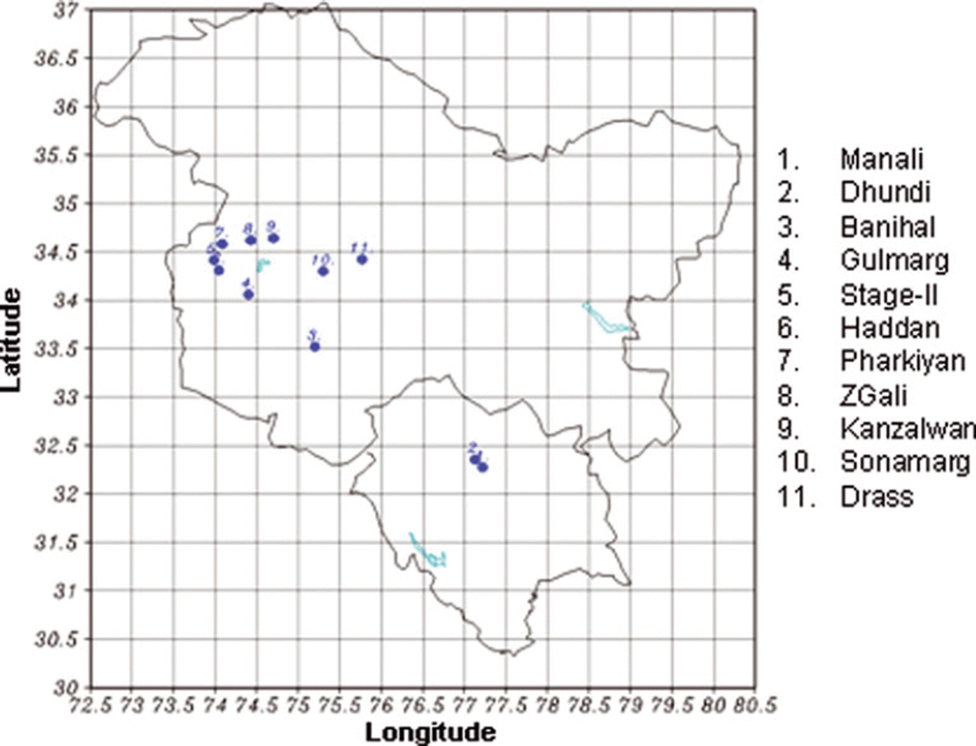
In this study, we explore the use of LAM forecasts as a means of making better predictions of key avalanche-relevant meteorological parameters (precipitation, 10 m wind speed and 2 m temperature) at 11 locations in the western Himalaya (Fig. 1). The 11 locations are where the Snow and Avalanche Study Establishment (SASE) of India maintains surface weather stations used to both study avalanche hazards and create avalanche-hazard forecasts for the area. The key scientific question addressed in this study is the problem of downscaling model forecast variables from the 10km × 10km grid resolution available from the LAM to the small surface-station scale, i.e. to conditions at the 11 surface stations. Our approach is to develop multiple linear regression formulae that express how surface station data are related to the model forecasts at 24, 48 and 72 hour lead times. These formulae are empirically based mappings between forecast variables on the 10km × 10km grid of the LAM and the data measured by the specific surface stations where accurate weather prediction for avalanche hazard assessment is required. The purpose of this paper is to describe the model, the data and the methods used to develop the multiple linear regression formulae.

Fig. 1. A map showing the 11 station locations for which the SDM has been developed.
Data and Methods
For the past three winter seasons, SASE has been using a LAM, the fifth-generation Mesoscale Model version 3.6 (MM5) (Reference Grell, Dudhia and StaufferGrell and others, 1995; Reference SrinivasanSrinivasan, 2006), to simulate avalanche-prediction related variables of the western Himalayan weather as a means of improving avalanche danger assessment. Each day, the LAM model provides a ‘prediction’ of weather variables at three future forecast times (24, 48 and 72 hours into the future) on a 10 km × 10 km grid of the study area. The three time series of daily forecasts are then compared with measured conditions at the 11 surface weather stations (Fig. 1) to create three sets of regression formulae. Each set of formulae represents the best estimator of the three key avalanche-prediction parameters (precipitation, 10 m wind speed and 2 m temperature) at each of the 11 stations using either day 1, day 2 or day 3 of the LAM forecast (24, 48 and 72 hours, respectively).
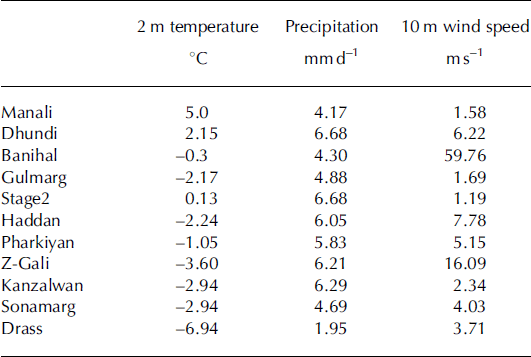
The model is run using a 30 km × 30 km ‘mother grid’ which contains a 10 km by 10 km ‘nested grid’. Each day, the model produces a 120 hour forecast simulation from which output is extracted and stored at 24, 48 and 72 hours. (Data at 96 and 120 hours were also stored, but were not used in this study.) Twenty-six parameters were extracted from the model forecasts to be used as predictors to develop the statistical equations. These parameters are listed in Table 1. The 26 predictors corresponding to 24, 48 and 72 hour forecast length are used to predict the parameters at respective forecast lengths. The observed data (predictands) collected over 11 surface weather stations of SASE (Fig. 1) were used to develop the regressions, and are summarized (by winter season averages) in Table 2. The 11 stations fall under lower Himalayan and middle Himalayan zones as characterized by Reference Sharma and GanjuSharma and Ganju (2000).
Table 1. Twenty-six parameters used to develop the statistical downscaling model (SDM)

Table 2. Climatological values of three parameters (averaged over four winter seasons) used in avalanche hazard assessment

In all, there are a total of 99 regression equations for three parameters at three different forecast hours (day 1, day 2 and day 3) over 11 stations. The model output data for three consecutive winters (November-April) from 2004 to 2007 were used to develop these multiple regression equations.
There are several approaches to the development of the statistical regressions (see, e.g., Reference Klein, Lewis and EngerKlein and others, 1959; Reference Glahn and LowryGlahn and Lowry, 1972). In our study, the selected 26 forecast predictors listed in Table 1 were made orthogonal and independent using the empirical orthogonal function (EOF) technique. Multiple linear regression analysis was then used to estimate the relationship between the predictands (the three variables at the 11 stations) and the principal components resulting from the EOF analysis. The multiple linear regression equation is given by
where Yis a vector of three components (the predictand), x is a vector of 26 components (the predictor) and the 3 × 26 rectangular matrix A is the matrix of regression coefficients that map x into Y. A separate matrix A is developed for each of the 11 stations. The goal of the method is to determine the matrix elements A using linear regression in order to minimize some performance index, such as J= (Y 0–Y). (Y 0 –Y) is the error between observation and prediction, where Y 0 are the observed values of Y derived from station data.
It is also important to evaluate the performance of the statistical model. This is accomplished by computing the root-mean-square error (RMSE) of the statistical downscaling model (SDM) developed with the above method and comparing the result with the intrinsic RMSE of the MM5 model itself. The comparison of the two RMSEs was done with the 3year dataset used for computing the regression coefficients, as well as with an independent dataset of the 2007/08 winter season derived from the same MM5 model output. The data from three consecutive winters (2004/05, 2005/06 and 2006/07) extracted from model output were used to develop the statistical model along with the observations. In order to test the developed SDM, an independent dataset of the 2007/08 winter of model output is reserved. RMSEs of the SDM were computed with both the three winter seasons’ data and the independent data of the 2007/08 winter. The results are discussed in the next section.
Results and Discussion
The computed RMSEs of the SDM, MM5 and observed standard deviation with respect to 24 hour forecast (day 1) of 2 m temperature, precipitation and 10m wind speed for the 11 stations are given in Figure 2. It is clear that the SDM shows a reduction in RMSE for all three parameters. RMSEs associated with the SDM are also less than the observed standard deviation (a measure of station weather variability), which shows that the SDM skill is acceptable as a means for improving the forecast at all 11 stations. Although the RMSE of the precipitation forecast is less than the observed standard deviation, the SDM RMSEs are comparable to the intrinsic variability of the MM5. For temperature and wind, the SDM shows good skills over MM5. Similar results were found for 48 hour forecast (day 2) and 72 hour forecast (day 3) regression formulae. For brevity these figures are omitted.

Fig. 2. Comparison of RMSEs of three parameters predicted by MM5 and the SDM, along with the observed standard deviation with respect to 24 hour forecast (day 1), computed with three consecutive winters’ data (2004/05, 2005/06, 2006/07).
In Figure 3, the computed RMSEs of the independent dataset (2007/08 winter) derived from the MM5 are compared with the SDM results. Even with the independent dataset, the SDM shows a reduction in RMSEs for all the stations relative to the forecast error of MM5. The SDM also shows a good model skill, except for wind at one station (Banihal; labelled 3 in Fig. 1). Statistically, if the computed RMSEs are less than the observed standard deviation, the performance/skill of the model in prediction is good. Similar results were observed for day 2 (48 hour) and day 3 (72 hour) forecasts of the parameters. For brevity, the figures corresponding to these results are not shown; however, the result indicates that use of a regression formula with any forecast, i.e. day 1, day 2 or day 3, provides a benefit for more accurate prediction of avalanche-related weather variables at the station locations.

Fig. 3. Same as Figure 2 but computed with independent dataset (winter season 2007/08).
With the 3 year dataset used for computing the regression coefficients, the RMSEs averaged over 11 stations for the 24 hour forecast of the three parameters are shown in Table 3. From this table it is evident that the reduction of RMSEs in the SDM over MM5 is beneficial and acceptable for two of the parameters, 2m temperature and wind; however, for precipitation the performance of the SDM is more marginal.
Table 3. Average RMSEs of the three parameters for 24 hour forecast (day 1) with different models.

Conclusion
In this study, we have demonstrated that a statistical regression approach to statistical downscaling (SDM) of MM5 model results yields significant improvements in the forecast of three avalanche-relevant weather parameters at 11 surface weather stations (field sites) where avalanche hazard prediction is needed on a day-to-day basis. The study demonstrates that SDM is superior to raw, unprocessed MM5 model results for forecasts extending 24, 48 and 72 hours into the future. While excellent results were obtained using the SDM for 10m wind speed and 2m temperature, forecast of precipitation using the SDM was more marginal, reflecting the local complexity of meteorological conditions in mountainous terrain. Overall, our study shows that detailed comparison of surface weather-station data, such as those collected by SASE for 11 sites in the western Himalaya, with limited-area weather-forecast models can yield statistically derived forecast improvements that can enhance the quality of avalanche hazard assessment.
Acknowledgements
We thank R.N. Sarwade, Director of SASE, for constant encouragement and support. The observational data used in this study were obtained from the archive of the Avalanche Forecasting Group, SASE. We thank M.S. Shekhar for providing valuable suggestions on the paper, and an anonymous referee for useful comments. We also thank D.R. MacAyeal for improving the readability of this paper substantially.


