


1. Introduction
Our knowledge of microwave penetration into snow on sea ice is inconsistent. In theory, penetration depth of microwaves is inversely (directly) proportional to frequency (wavelength). In addition, microwave penetration into snow is affected by the interplay between scattering and absorption, which in turn depends on the physical properties of snow, such as surface roughness, stratigraphy, density, grain size and shape, salinity and wetness. Of particular interest has been the Ku band frequency (~13.6 GHz) that is used by many past, present and proposed satellite radar altimeter missions, such as ERS-1/2, Envisat, CryoSat-2, Sentinel-3A/B and CRISTAL (Quartly and others, Reference Quartly2019). Using their data for freeboard retrieval and the freeboard-to-thickness conversion in sea-ice thickness measurements relies on the assumption that the Ku band radar return penetrates the snow cover and originates from the sea-ice surface. Generally, it is also assumed that the higher frequency band radar signals, such as from the Ka band radar altimeter onboard the AltiKa satellite mission (35.75 GHz), do not penetrate the snow cover but are reflected from the snow surface. These assumptions of differences in penetration depth set the premise for satellite-based dual-frequency snow depth retrieval (Guerreiro and others, Reference Guerreiro, Fleury, Zakharova, Rémy and Kouraev2016; Lawrence and others, Reference Lawrence, Tsamados, Stroeve, Armitage and Ridout2018; Garnier and others, Reference Garnier2021).
It has been shown in a laboratory that for a cold, dry, homogeneous, 21 cm-thick snow cover, the snow–ice interface return indeed dominated and the snow volume scatter contribution was negligible at the Ku band (Beaven and others, Reference Beaven1995). However, both field observations and modelling studies suggest that the assumption may be invalid outside laboratory conditions due to the more variable properties of natural snowpack on sea ice (e.g. Barber and others, Reference Barber, Reddan and LeDrew1995; Willatt and others, Reference Willatt, Giles, Laxon, Stone-Drake and Worby2010, Reference Willatt2011; Nandan and others, Reference Nandan2017; Landy and others, Reference Landy, Petty, Tsamados and Stroeve2020; Nandan and others, Reference Nandan2020). Roughness of the snow surface, especially at microwave wavelengths in millimetre to centimetre scale that are close to the roughness length scales, is known to increase the proportion of diffuse scattering affecting the measured backscatter. In particular, over first-year ice, the bottommost layers of the snowpack may be wetted with brine strongly increasing the attenuation and thus reducing the penetration of microwaves. Changes in temperature affect the brine volume and salinity and, if increasing close to the melting point, even enable existence of liquid water further altering and complicating backscatter behaviour (Ulaby and Long, Reference Ulaby and Long2014). Due to their smaller footprint size, observations from ground-based radar systems are required not only to understand how different snow and sea-ice types affect the backscattered radar signal and from where the dominant scattering originates but also to interpret the measurements from other radar platforms correctly. Due to their larger footprint size, radar observations from aircraft and satellites can often include contributions from a mixture of surface types whereas a ground-based system can target a single homogeneous surface and assist in decomposing the backscatter signal (Stroeve and others, Reference Stroeve2020).
There is an abundance of studies focusing on microwave penetration into snow using ground-based frequency-modulated continuous-wave (FMCW) radars (e.g. Marshall and Koh, Reference Marshall and Koh2008, and references therein). They focus mostly on frequencies at or lower than the Ku band and on terrestrial snow while similar studies using higher frequencies, such as the K or Ka band, or focusing on snow on sea ice are scarce. One example including higher frequencies is the study by Koh and others (Reference Koh, Yankielun and Baptista1996), where multiband FMCW radars at C (3.9–5.9 GHz), X (8.2–12.4 GHz) and Ka (26.5–40 GHz) bands were used to characterise the snow cover in terrestrial test sites in the Northeastern USA. It was demonstrated that the higher frequencies were more sensitive to the snow microstructure revealing subtle changes between layers while sometimes unable to detect the ground reflection. The lower frequencies were more suitable for studying deeper and wetter snowpacks.
Many previous ground-based radar studies covering topics such as microwave backscatter and extinction mechanisms as well as determining snow thickness on sea ice have concentrated on the Antarctic. Snow cover on the Antarctic sea ice is generally deeper and more complex compared to the Arctic due to warmer winter temperatures, frequent flooding and strong metamorphism in summer. Kanagaratnam and others (Reference Kanagaratnam2007) studied snow on the Antarctic sea ice with an S/C band (2–8 GHz) FMCW radar finding the air–snow and snow–ice interfaces dominating the radar echoes and a high correlation between in situ and radar-derived snow depths. Willatt and others (Reference Willatt, Giles, Laxon, Stone-Drake and Worby2010) extended the bandwidth to higher frequencies by using a C/X/Ku band (4.5–16 GHz) FMCW radar to study radar response from different snow types also in the Antarctic. They found that the assumption of the snow–ice interface returns dominating at Ku band was valid for the surveyed sea ice in the Antarctic only when stratigraphic features and flooding were absent. Using an airborne radar altimeter in the Arctic, Willatt and others (Reference Willatt2011) showed that Ku band microwaves did not penetrate as deep but were reflected closer to the air–snow interface when the snow temperature was relatively warm, i.e. close to melting (up to $-4^\circ$ C). More recently, a fully polarimetric and dual-frequency, Ku (12–18 GHz) and Ka (30–40 GHz) band, FMCW radar was deployed on the Arctic sea ice during the year-long Multidisciplinary drifting Observatory for the Study of Arctic Climate (MOSAiC) drift expedition in 2019–20 (Stroeve and others, Reference Stroeve2020; Nicolaus and others, Reference Nicolaus2022). Related studies have found potential in the dual-frequency approach to derive snow thickness (Stroeve and others, Reference Stroeve2020) but also factors complicating the analysis of waveforms and backscatter such as rain-on-snow events (Stroeve and others, Reference Stroeve2022), wind redistribution of snow leading to densification at the surface, as well as existence of previous air–snow interfaces (Nandan and others, Reference Nandan2022).
The studies mentioned above and many others alike have been conducted with purpose-built FMCW radars. Using FMCW technology combined with a wide bandwidth rather than conventional pulsed radars is beneficial for acquiring better range resolution, but it may bring unwanted complexity to the radar system and increased development costs. In recent years, using commercial radars has become increasingly popular for their ease of use and relatively low cost. Low-frequency ground-penetrating radar (GPR) is a well-established method in studying glaciers (Navarro and Eisen, Reference Navarro and Eisen2009) and the seasonal snow cover especially in the Nordic countries (Lundberg and others, Reference Lundberg, Granlund and Gustafsson2010). Pfaffhuber and others (Reference Pfaffhuber, Lieser and Haas2017) pulled off-the-shelf, 400 and 800 MHz GPRs in a sledge over the Antarctic sea ice and argued that GPRs are efficient in snow thickness surveys and ‘thus, making purpose-developed, complicated step frequency/frequency-modulated radars is not strictly necessary for the task’. The usage of commercial FMCW radars in snow research is still in its infancy as technology continues to become more affordably available, but recently Pomerleau and others (Reference Pomerleau2020) demonstrated the use of an off-the-shelf, 24 GHz FMCW drone-mountable radar in measuring lake ice thickness and monitoring snow water equivalent (SWE) and snow density (snow depth was determined by other means). Other types of ultra-wideband radar, albeit often custom-developed, have recently been deployed on drone platforms (e.g. Jenssen and Jacobsen, Reference Jenssen and Jacobsen2021; Tan and others, Reference Tan, McCulloch, Rack, Platt and Woodhead2021). Such small and easy-to-use radars would be beneficial to integrate with other instruments: one appealing application being the electromagnetic induction sounding instrument (EM-Bird; Haas and others, Reference Haas, Lobach, Hendricks, Rabenstein and Pfaffling2009) to enable simultaneous measurements of the snow and sea-ice layer thicknesses.
This study investigates the penetration of C (6 GHz) and K (26 GHz) band microwaves into snow on sea ice using field experiments with commercial pulsed tank radars aided by detailed surveys of snow stratigraphy. The measurements were conducted over landfast first-year and multiyear Arctic sea ice in May 2018. The objectives are the following: (1) to determine the locations of the dominant scattering surfaces for each of the two frequencies and relate them to the structure and physical properties of the snow cover, (2) to assess a hypothesis that snow depth could be derived from the difference of C and K band measurements, and (3) to explore if off-the-shelf, conventional pulsed radars and their software are feasible for the purpose of snow depth retrieval.
2. Data and methods
2.1. Study site and general conditions
The field campaign of the 2018 Multidisciplinary Arctic Program – Last Ice took place on landfast sea ice in the Lincoln Sea ~6 km off the coast of Ellesmere Island near Canadian Forces Station (CFS) Alert in May 2018 (Figs 1a–c). The landfast sea ice was composed of multiyear ice (MYI) pack ice floes that had become landfast and first-year ice (FYI) formed inbetween during the winter 2017–18. The study site was chosen so that both FYI and MYI were easily accessible (Lange and others, Reference Lange2019). During the field measurements, the mean air temperature was −9 ± 4°C and the following major weather events were observed: wind-driven snow redistribution event on 9–10 May, freezing drizzle on 15 May and snowfall without significant redistribution by wind on 22–23 May (Fig. 1d). Using a ground-based electromagnetic (EM) induction sounding instrument (Geonics EM31SH; method described in Haas and others, Reference Haas2017), the measured sea-ice thickness values along a 240 m long transect crossing both ice types on 24 May were on average 1.4 ± 0.2 m for FYI and 2.9 ± 0.7 m for MYI. Snow thickness was measured along the same transect on 9–10 May before the snowfall event using an automatic snow depth probe (Snow-Hydro LLC magnaprobe; Sturm and Holmgren, Reference Sturm and Holmgren2018) resulting in average values of 0.22 ± 0.12 m and 0.42 ± 0.24 m for FYI and MYI, respectively. After the snowfall event, the average snow depths had increased by 5–8 cm to 0.30 ± 0.12 m and 0.47 ± 0.23 m for FYI and MYI, respectively, as measured on 24 May (Lange and others, Reference Lange2019). Moreover, aircraft surveys by NASA Operation IceBridge (OIB) were carried out over the study site prior to the field campaign on 4 and 16 April 2018 (Studinger and others, Reference Studinger, Young and Larsen2011; NASA, 2018). Here, only the airborne optical imagery is used for illustrative purposes due to the long time interval between the airborne and in situ campaigns and the fact that data from some airborne instruments, such as the snow radar, did not cover the entire areal extent of the ground measurements due to adverse weather conditions and the proximity of the coastline.

Figure 1. (a) The study site in Alert in the Arctic-wide context together with the sea-ice area fraction on 5 May 2018 from the OSI SAF Global Sea Ice Concentration Interim Climate Data Record Release 2 product (OSI SAF, 2020). (b) The main ice camp (red square, the extent of panel (c)) in relation to Ellesmere Island and the Canadian Forces Station (CFS) Alert (red diamond) on a Sentinel-1A level-1 interferometric wide swath (IW) ground range detected (GRD) high-resolution HH-polarised SAR image acquired in the beginning of the field campaign on 3 May 2018 as well as two snow study locations (red dots) on a big MYI floe. The orange line is the NASA Operation IceBridge (OIB) flight track on 16 April 2018 (NASA, 2018). Brighter colours of the SAR image indicate higher backscatter, i.e. rougher (or older) sea ice, and darker colours lower backscatter, i.e. smoother (or younger) sea ice. Copernicus Sentinel data 2018. (c) The detailed snow study locations (red dots) close to the main ice camp on OIB Digital Mapping System (DMS) optical imagery from 4 April and 16 April 2018 (Dominguez, Reference Dominguez2010). The numbering of snow study locations in (b) and (c) refers to Table 1. The red dashed line shows the approximate border between FYI and MYI. (d) Hourly air temperature (red, left-hand side) and snow depth (black, right-hand side) in May 2018 measured by Snow Buoy 2018S65 (Grosfeld and others, Reference Grosfeld2015; Katlein and Nicolaus, Reference Katlein and Nicolaus2019; Nicolaus and others, Reference Nicolaus2021) deployed close to the snow pit #2 (MYI buoy) in panel (c). Grey background indicates the period of detailed snow studies. Moreover, major weather events, such as freezing drizzle observed on 15 May and snowfall on 22–23 May, are marked.
Table 1. Summary of the detailed snow studies including instruments and parameters

aOne day later.
bCoarse (20–25 cm) lateral resolution.
cData saving failure.
dOnly radar and h s also on 11, 13, 15, 17, 19, and 22 May 2018.
eOnly radar and h s also on 17, 19, and 22 May 2018.
The numbering refers to Figure 1. h s is snow depth, SMP is the SnowMicroPen instrument, T s is snow temperature, ρ s is snow density, SSA is specific surface area using the IceCube instrument, F is snow grain shape/form, E is snow grain size, R is snow hardness and S is salinity. Symbols follow Fierz and others (Reference Fierz2009). The last column indexes the figures summarising the measurement results.
2.2. Detailed snow studies
The detailed snow studies took place between 11 and 24 May as summarised in Table 1. A total of nine locations were studied, divided roughly equally between FYI and MYI, including two locations with repeated visits to create a short time series of the radar response over up to 13 days. The measurement procedure consisted first of non-destructive radar measurements and then successive destructive auxiliary snow measurements. They are summarised in the list below and explained in more detail in the following subsections.
1. Radar measurements
2. Auxiliary snow measurements
(a) High-resolution snow penetrometer measurements
(b) Snow pit measurements
i. Temperature
ii. Density
iii. Specific surface area (SSA)
iv. Stratigraphy, including snow grain type and size as well as hand hardness
v. Salinity
2.2.1. Radar measurements
The radars used for studying microwave penetration were commercial, off-the-shelf Endress+Hauser Micropilot radars FMR54 (C band, ~6 GHz) and FMR51 (K band, ~26 GHz). Their main parameters are summarised in Table 2. Such radars are commonly used in industrial applications for continuous monitoring of a material level in a tank, hence the devices are often called tank radars. Unfortunately, there is little expert information on these commercial radars provided by the manufacturer (Endress+Hauser, 2018a, 2018b): The FMR54 and FMR51 are ‘downward-looking’ measuring systems, operating based on the time-of-flight (ToF) method. They measure the distance from the reference point (process connection) to the product surface. Radar pulses are emitted by an antenna, reflected off the product surface and received again by the radar system. The reflected radar pulses are received by the antenna and transmitted into the electronics. A microprocessor evaluates the signal and identifies the level echo caused by the reflection of the radar pulse at the product surface. The unambiguous signal identification is accomplished by a proprietary software ‘PulseMaster® eXact’ together with the Multi-echo tracking algorithms, based on many years of experience with ToF technology. The distance D to the product surface is proportional to the time of flight t of the impulse:

with c being the speed of light. The Micropilot is equipped with functions to suppress interference echoes. The user can activate these functions. Together with the multi-echo tracking algorithms, they ensure that interference echoes (i.e. from edges and weld seams) are not interpreted as level echo. We used the radars in the mode ‘workbench test’ which ensures that all filtering and smoothing parameters were turned off and the outputted envelope curves were as close as possible to the raw data curve.
Table 2. Summary of the radar parameters reported by the manufacturer Endress+Hauser

aIn diameter, beam-limited, range 1 m/1.5 m.
bPlastic housing.
cAntenna and process connection.
dStainless steel flange.
eHighway addressable remote transducer.
First, a mostly wooden instrument stand was carefully placed over an untouched snow cover (Fig. 2a). The distance of the legs was 1 m, i.e. wider than the footprint of the radars (Table 2). The stand had two crossbars for supporting radar measurements at heights of ~1 and 1.5 m, depending on the bearing capacity of the snow cover. The configuration assured that all measurements were carried out with near nadir incidence angles, deviating by no more than a few degrees. This is important as larger deviations from nadir could result in spurious results due to changing surface scattering contributions on the one hand, and due to the effects of potential radar beam side lobes. However, other than the beamwidths stated in Table 2 not much other information is provided by the manufacturer (Endress+Hauser 2018a, 2018b): The beam angle is defined as the angle α where the energy density of the radar waves reaches half the value of the maximum energy density (3 dB-width). Microwaves are also emitted outside the signal beam and can be reflected off interfering installations. However, in many applications, the radars are installed in stilling wells and bypass pipes that are not wider than the antennas, which leads us to assume that the effects of sidelobes are small if the data are acquired near nadir.

Figure 2. (a) Photograph illustrating the setup using the FMR51 and FMR54 radars. R is range from the radar flange, h s is snow depth, and the dashed line across the radar footprint shows the SnowMicroPen (SMP) measurement line. Radars were used one at a time. (b) Snow pit #4 MYI OIB on 18 May 2018 (Fig. S3) while measuring the temperature profile overlaid with annotations of different snow layers. The dashed lines indicate approximate transitions between layers. The inset in the lower-right corner of the photo illustrates the centimetre-scale depth hoar crystals that were found in the lower layers.
The radar measurements were recorded using the manufacturer's licensed FieldCare software on a laptop computer. The software outputted an envelope of the returned power (in decibel units, dB) internally constructed from the received pulses and as a function of distance from the radar flange (zero level). To verify the reproducibility and representativity of the measurements, the measurements were taken with one radar first at the lower 1 m height, then at the higher 1.5 m height, repeated at the lower height and then duplicated with the other radar. During the first radar measurement at each measurement height, the range to the snow surface was recorded with a ruler to compare the location of the air–snow interface in the radar data. After the radar measurements were done, the radars and the instrument stand were carefully removed with minimal disturbance to the snow.
In addition, we carried out a snow removal experiment on first-year ice where measurements were repeated at different heights over the bare ice surface after the snow was removed. Figure 3 shows an example of those measurements from the snow pit #7 FYI transect on 22 May 2018 (see Fig. 4 of measurements with snow for comparison). The manually measured ranges to the exposed smooth FYI surface were 1.22 m for the lower measurement height and 1.72 m for the higher measurement height. The radar measurements show very similar responses for both C and K band radars and the peaks align within 0–2 cm of the manual range measurements. Taking into account the range resolutions of the radars (~2–3 cm) and the accuracy of the manual range measurements with a ruler (0.5 cm), there is no systematic offset between the radar and manual range measurements. Eventually, it would be good to have better information about the actual impulse response for interpretation or for deconvolving the radar response. However, these require more information on important aspects of the radar parameters and internal processing from the manufacturer but are undisclosed.

Figure 3. Measurements with the C band (red) and K band (black) tank radars at the lower (solid) and higher (dashed) measurement height after clearing the snow below the wooden measurement stand at snow pit #7 FYI transect on 22 May 2018. The horizontal grey lines show the range to the exposed sea-ice surface measured manually with a ruler.

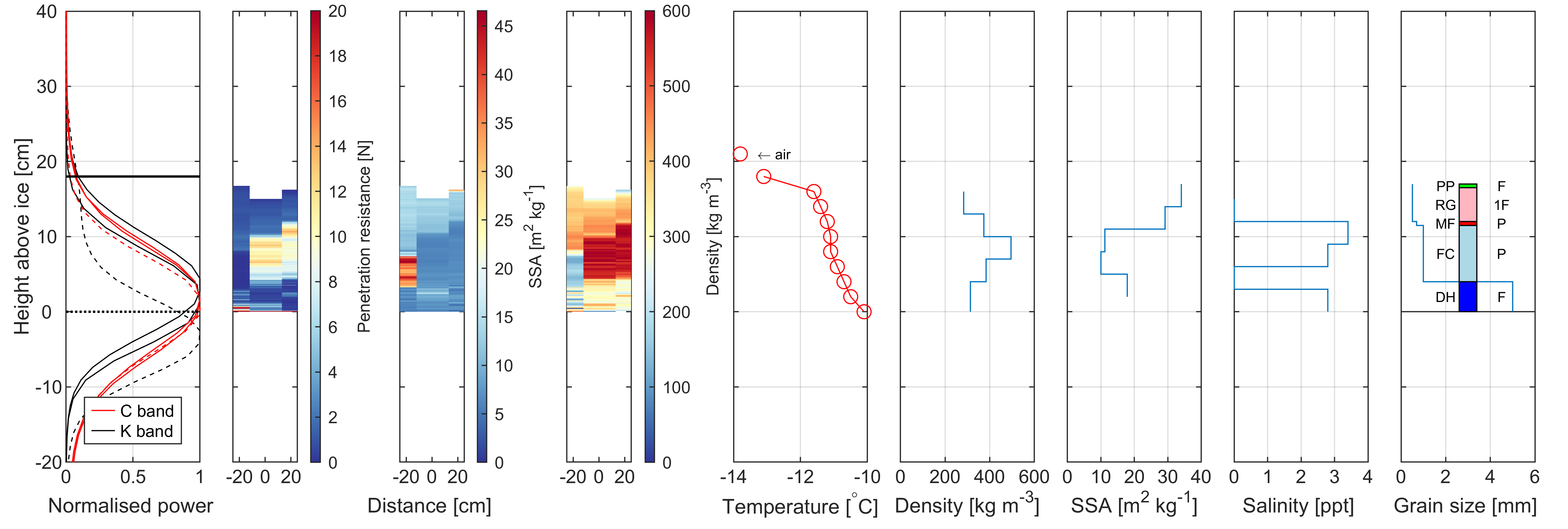
Figure 4. Snow pit #7 FYI transect on 22 May 2018. (a) The first panel shows the normalised radar returns for C (red) and K bands (black) and for the lower (solid) and higher (dashed) measurement height with the horizontal lines marking the snow (solid) and sea-ice (dotted) surfaces. The next three panels show the SnowMicroPen measurements across the radar footprint, where zero distance indicates directly under the radar at the middle of the instrument stand and positive distance is to the right. (b) Standard snow pit measurements. SSA stands for specific surface area. Letter and colour code for snow grain type: precipitation particles (PP), Lime; decomposing and fragmented precipitation particles (DF), forest green; rounded grains (RG), light pink; faceted crystals (FC), light blue; depth hoar (DH), blue; melt forms (MF), red; ice formations (IF), cyan. Letter code for hand hardness: very soft, F (fist); soft, 4F (4 fingers); medium, 1F (1 finger); hard, P (pencil); very hard, K (knife blade); ice, I (ice) (Fierz and others, Reference Fierz2009).
At two study locations, called FYI temporal and MYI temporal, the radar measurements were repeated every other day in the exact same location to record short time series of the radar response and, therefore, only snow depth was recorded with a thin metal probe. The more destructive auxiliary snow measurements consisting of penetrometer and snow pit measurements, described in the following paragraphs, were done only on the last sampling day.
2.2.2. Auxiliary snow measurements
A high-resolution snow penetrometer, SnowMicroPen (SMP; Schneebeli and others, Reference Schneebeli, Pielmeier and Johnson1999), was used to sample the snow cover along a short transect across the radar footprint laterally every 10–25 cm (dashed line in Fig. 2a). The SMP measures high-resolution profiles of penetration force when the measurement tip at the end of a metal rod is driven with constant speed vertically into the snowpack. Proksch and others (Reference Proksch, Löwe and Schneebeli2015) empirically linked the penetration force to physical snow properties, such as density and specific surface area (SSA, surface area per unit mass). SSA is inversely proportional to the effective snow grain size, i.e. the diameter of spherical scatterers (e.g. Gallet and others, Reference Gallet, Domine, Zender and Picard2009); therefore, the larger the SSA, the smaller are the snow grains, and vice versa. These derivatives are used here only for illustrative purposes, as recalibration might be necessary for the snowpack on the Arctic sea ice but also due to instrument hardware updates (Proksch and others, Reference Proksch, Löwe and Schneebeli2015; King and others, Reference King2020) but that is out of scope for this study. Therefore, we use Proksch and others (Reference Proksch, Löwe and Schneebeli2015) instead of King and others (Reference King2020) in this study.
After the SMP measurements, the disturbed snow was cleared and a vertical wall of snow, i.e. a snow pit, was prepared in a way that it was shadowed from direct sunlight (Fig. 2b). First, a snow temperature profile was recorded using a digital thermometer (testo 110 with a stainless steel food probe) in 2–5 cm vertical resolution. Second, snow density measurements were carried out by extracting 100 cm3 (6 cm × 3 cm × 5.5 cm) samples of snow using a light-weight box cutter (also known as the Taylor–LaChapelle cutter) in 3 cm vertical resolution and weighing them on a digital scale. Third, snow SSA was determined in 3 cm depth intervals using the IceCube instrument (A2 Photonic Sensors; Gallet and others, Reference Gallet, Domine, Zender and Picard2009). Fourth, snow stratigraphy was resolved based on snow grain shape and average size, determined with a crystal card and a magnifying glass, and a hand hardness test by the observer. The grain shape and hardness scales follow the International Classification for Seasonal Snow on the Ground (Fierz and others, Reference Fierz2009). Last, a snow salinity profile was measured from samples of snow collected in 3–5 cm resolution to plastic bags. The samples were allowed to melt in a heated tent and salinity was determined using the WTW Conductivity portable meter ProfiLine Cond 3110.
For the analysis, the radar measurements were vertically aligned with the SMP and snow pit measurements using the manually measured range between the radar and the snow surface. The vertically averaged bulk density of snow (ρ ds) from the box cutter measurements was used for calculating the propagation speed of the radar wave in snow (c s) to adjust the radar range in snow:

where n s is the refractive index of snow (Ulaby and Long, Reference Ulaby and Long2014). The radar return power was converted to linear scale and normalised to the maximum power for readily determining of the dominant scattering horizon. The location of the maximum power (normalised power equals 1) was taken as the location of the main scattering horizon.
3. Results and discussion
In all snow pits, the observed general structure of the snow cover was typical for Arctic sea ice. Closest to the snow–ice interface was a low-density layer of large-grained depth hoar underlying a wind slab layer with smaller, rounded grains and higher density (Fig. 2b). Many of the studied snowpacks had a layer of melt forms or even an ice lens in them indicating an occurrence of a warmer period earlier that winter. Freezing drizzle on 15 May created a thin, icy crust on the surface and snowfall on 22–23 May brought up to 10 cm of very soft, new snow on top. In general, the snow cover on FYI was relatively thin, on average just 22.5 cm. On FYI, the bottommost layers reached up to 12 ppt in salinity, whereas snow on MYI was thicker at 43.4 cm on average but fresh (non-saline).
During the measurement period 11–24 May, the air temperature rose from $-18^\circ$ C to close to melting point, $-0.9^\circ$
 C (Fig. 1d). Temperatures above $-5^\circ$
 C increase the possibility of liquid water presence in the snow cover and subsequently, also the possibility of changes to the dielectric properties of snow. However, liquid water content (LWC) profiles were not included as part of the detailed snow studies as the obtained measurements were deemed unreliable.
In this section, two example cases of the detailed snow studies together with the longer time series of radar response are presented and discussed. The examples represent two cases with different than expected and opposing radar behaviour. The remaining figures that summarise the measurements are included in the supplementary material of this manuscript and indexed in Table 1.
The first example in Figure 4 shows the measurements carried out on the snow and sea-ice thickness transect, i.e. at the location called snow pit FYI transect (see #7 in Fig. 1c), on 22 May and represents the expected radar behaviour. From a 20 cm-thick snow cover, the main scattering horizon for the C band radar originated exactly from the snow–ice interface whereas the K band microwaves were reflected from the air–snow interface regardless of the measurement height indicating good reproducibility of the radar measurements. The difference in the range-corrected distance between the peaks of the two frequencies was 20 cm and in excellent agreement with the snow depth. Both radar frequencies seemed surprisingly unaffected by the high salinity of 12 ppt in the bottommost 10 cm of the snowpack and the relatively warm snow temperature ranging from −6 to $-3^\circ$ C, as increased salinity and temperatures close to melting have been reported to increase microwave absorption and to shift the main scattering horizon upwards. For comparison, see Figure 3 for snow removal experiment measurements at this snow pit location.
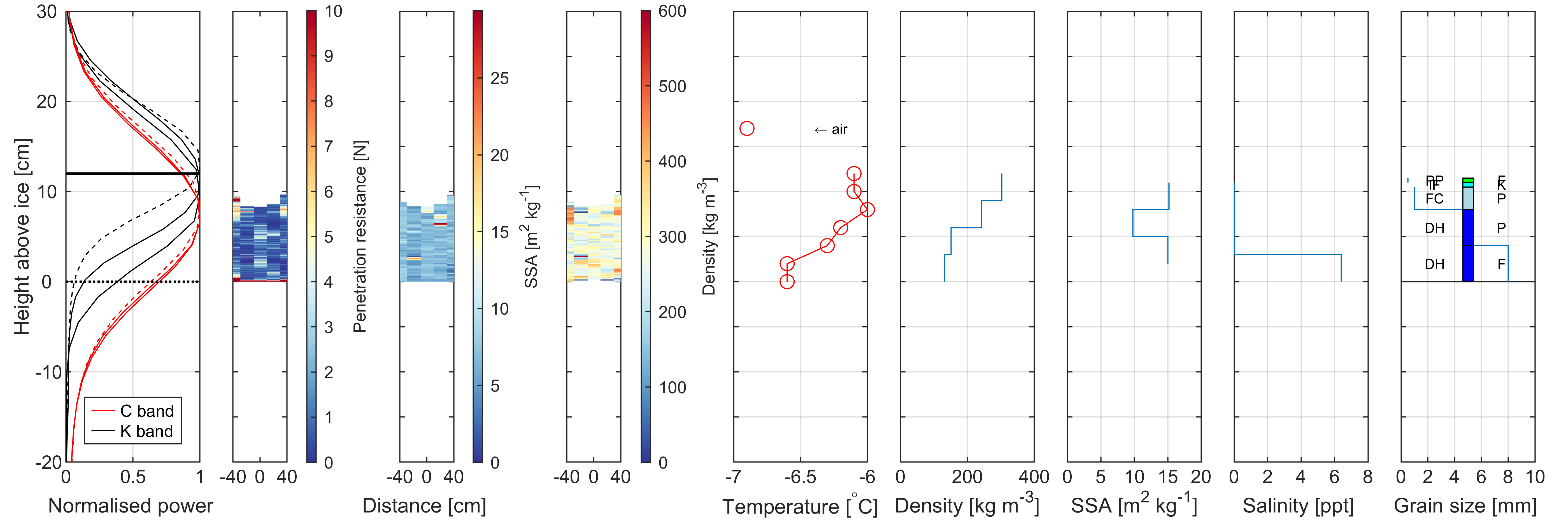
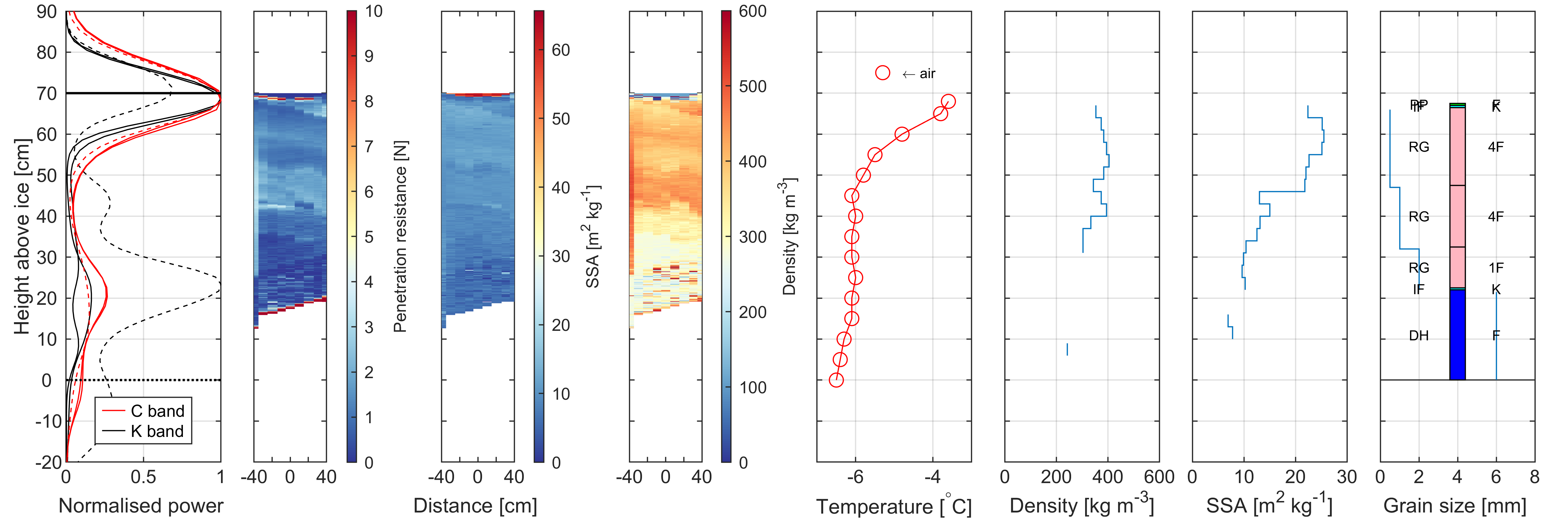
In contrast, the measurements of the second example case conducted at the snow pit #2 MYI buoy on 14 May are shown in Figure 5. Here, the radar measurements were affected by a few centimetres thick, high-density icy layer ~20 cm above the snow–ice interface. All but one of the radar returns placed the main scattering horizon to this layer or slightly above it. For an unknown reason, the C band measurement from the higher measurement height had the strongest return about 15 cm higher than the respective K band measurement, although similar in shape, placing it above the air–snow interface (see dashed red line). This particular measurement was regarded erroneous. In addition, it must be noted that the thickness of the snow cover directly under the radar was about 32 cm and increasing from left to right, but as the disturbed snow was cleared for the snow pit measurements, the resulting height of the snow pit wall was 42 cm due to small-scale ice surface roughness and related change in snow depth within the radar footprint.

Figure 5. Snow pit #2 MYI buoy on 14 May 2018. (a) The first panel shows the normalised radar returns for C (red) and K bands (black) and for the lower (solid) and higher (dashed) measurement height with the horizontal lines marking the snow (solid) and sea-ice (dotted) surfaces. The next three panels show the SnowMicroPen measurements across the radar footprint, where zero distance indicates directly under the radar at the middle of the instrument stand and positive distance is to the right. Note that snow depth for the radars and penetrometer was about 10 cm less than for the snow pit measurements (top). (b) Standard snow pit measurements. SSA stands for specific surface area. Letter and colour code for snow grain type: precipitation particles (PP), lime; decomposing and fragmented precipitation particles (DF), forest green; rounded grains (RG), light pink; faceted crystals (FC), light blue; depth hoar (DH), blue; melt forms (MF), red; ice formations (IF), cyan. Letter code for hand hardness: very soft, F (fist); soft, 4F (4 fingers); medium, 1F (1 finger); hard, P (pencil); very hard, K (knife blade); ice, I (ice) (Fierz and others, Reference Fierz2009). The salinity profile is not shown, because all MYI snow pits had zero salinity.
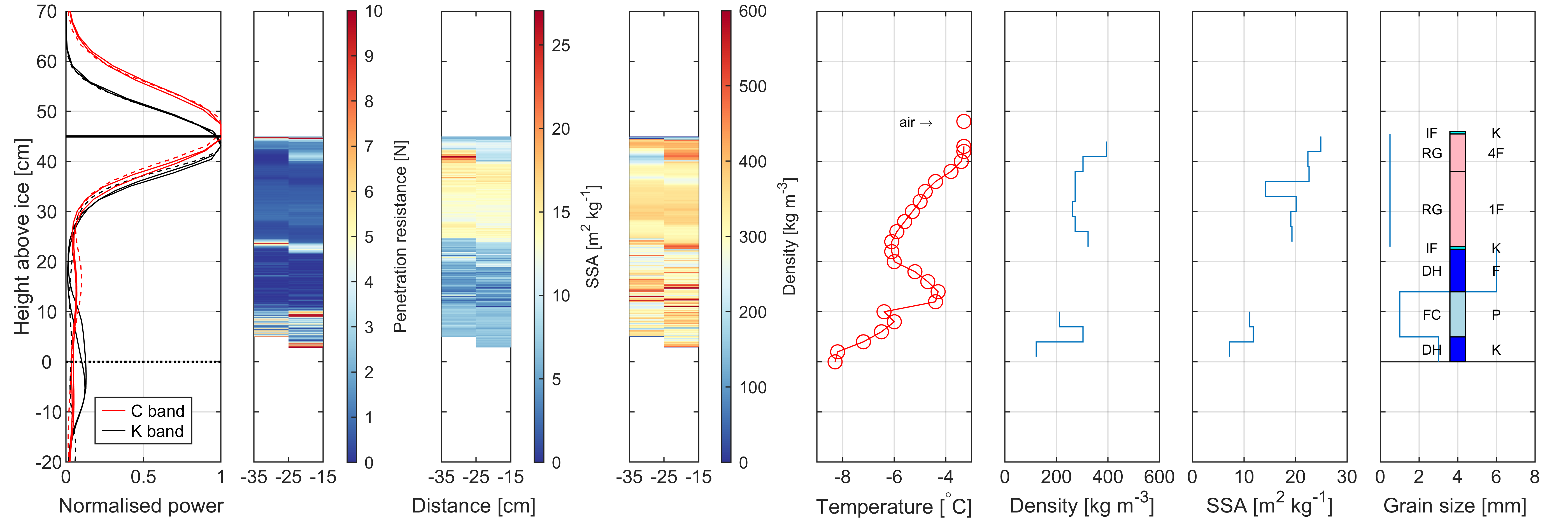
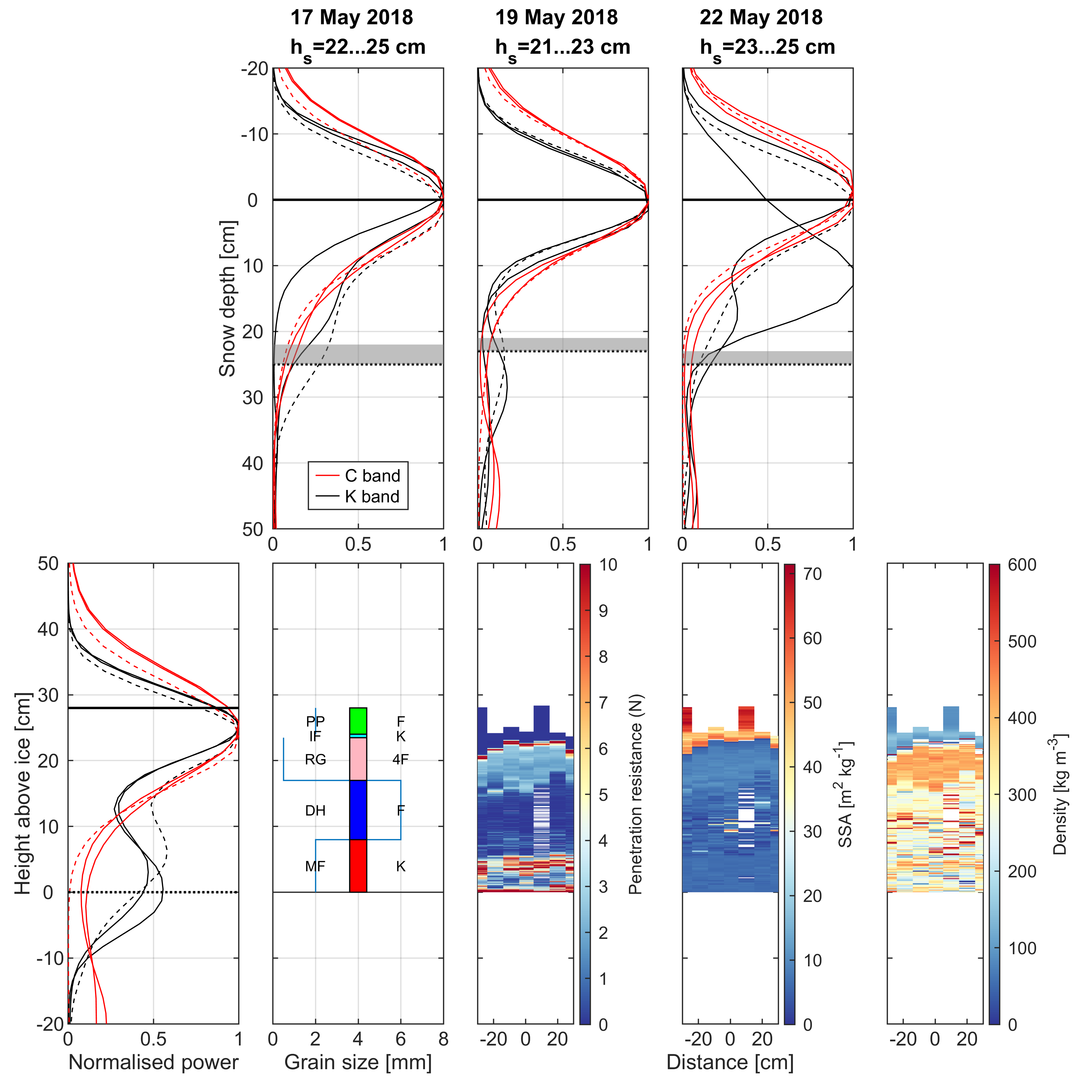
Figure 6 shows the temporal evolution of the radar return signals from the exact same snow at the study location #8 FYI temporal. Note, this is not the same location (#7) as the FYI observations plotted in Figure 4. In the beginning of the time series on 11 May, the higher-frequency K band microwaves reflected from or slightly below the air–snow interface whereas the lower-frequency C band microwaves expectedly penetrated deeper. However, the C band main scattering horizon seemed to correspond to a high-density layer of melt forms, which was located at 7 − 13 cm above the ice surface in the snow pit measurements on 24 May, rather than to the snow–ice interface. Later on by 22 May, the location of the strongest C band return had migrated upward to less than 10 cm below the snow surface. The K band penetration into snow was even more variable with the dominant scattering horizon changing between the snow surface and the melt form layer or both showing double-peak behaviour. Also opposing behaviour depending on the measurement height was observed for both radars, on 17 May for K band and on 19 May for C band. Very likely reasons for the decrease in penetration depth could be the increased snow temperature (air temperature peaked at $-0.9^\circ$ C on 19 May, Figure 1d) and possible wetness of the snow cover during the measurement period. Unfortunately, neither of those parameters were measured at this study location to avoid disturbing and destructing the snowpack. The 15 cm-thick new snow, which accumulated during the snowfall on 22–23 May, remained mostly undetected by the radars due to its very low density and thus, the lack of dielectric contrast between air and snow. The top layers consisted of (fragmented) precipitation particles and were so soft that only one of the SMP measurements captured the full profile, while for most of them the instrument did not register enough resistance.

Figure 6. Measurements at the study location #8 FYI temporal. (Top) Repeated C (red) and K band (black) radar measurements for the lower (solid) and higher (dashed) measurement height between 11 and 22 May 2018 without detailed snow pit measurements. Note that the vertical axis is normalised to the snow surface and converted into snow depth. Range of snow depth values probed under the radar are indicated above each panel and as grey transparent boxes. (Bottom) Radar measurements on 24 May 2018 followed by stratigraphy and penetrometer measurements. The closest hourly air temperature values from the nearby Snow Buoy 2018S65 (T air, Figure 1d) are given with the radar measurements. SSA stands for specific surface area. Note that the vertical axis is now normalised to the ice surface. Letter and colour code for snow grain type: precipitation particles (PP), lime; decomposing and fragmented precipitation particles (DF), forest green; rounded grains (RG), light pink; faceted crystals (FC), light blue; depth hoar (DH), blue; melt forms (MF), red; ice formations (IF), cyan. Letter code for hand hardness: very soft, F (fist); soft, 4F (4 fingers); medium, 1F (1 finger); hard, P (pencil); very hard, K (knife blade); ice, I (ice) (Fierz and others, Reference Fierz2009). The photograph in the bottom right corner shows a close-up of the SnowMicroPen instrument and illustrates the softness of the topmost layers.
In summary, the radars were operated at nine locations recording a total of 108 radar returns divided equally between the C and K band frequencies and in 2:1 ratio between the lower and higher measurement height. For the C band radar, the dominant scattering surface was closer to the air–snow interface in 54% of the returns, including all MYI snow pits. In 39% of the returns, all in snow on FYI, the strongest signal originated closer to the snow–ice interface. A minority (7%) of the dominant scattering horizons seemed to be located above the snow surface (Fig. S4) indicating perhaps a measurement error due to possible, unrecorded movement of the instrument stand into the snow under the weight of the heavy radars. However, this was still within the range resolution of the radars (about 2.9 cm for the C band radar and about 2.2 cm for the K band radar). For the K band radar, a clear majority (81%) of the dominant returns were located within the range resolution distance of 2–3 cm to the air–snow interface, whereas a small fraction (17%) originated closer to the snow–ice interface. One single return was located a few centimetres below the snow–ice interface within the sea ice (Fig. S1).
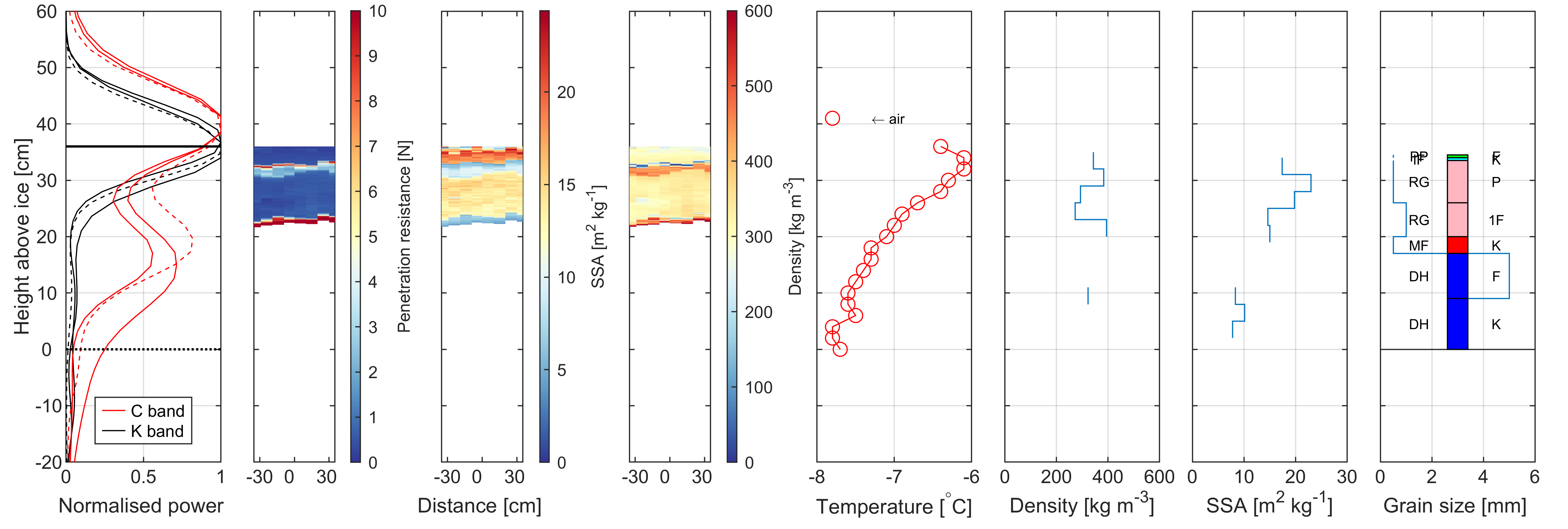
Altogether, the analysis of microwave penetration was challenging and very dependent on the prevailing conditions. All studied snowpacks had some stratigraphic features, such as a surface crust, an ice lens, a melt form layer of varying thickness or depth hoar, that may have influenced the radar wave propagation and originated from previous autumn. Additionally, the air temperature was close to or even above $-5^\circ$ C for the majority of the study period increasing the possibility of liquid water and resulting microwave absorption in the snowpack (Barber and others, Reference Barber, Reddan and LeDrew1995). Further insights and assistance in interpreting the radar returns and backscattering behaviour could be gathered from supporting measurements of surface roughness and LWC that should be collected in future measurement campaigns. Further inaccuracies may arise from radar mispointing off-nadir and the radar parameters allowing a range resolution of ~3 cm. Inarguably, FMCW radars would have been able to acquire more detailed radar profiles increasing the sensitivity to thin layers (Marshall and others, Reference Marshall, Schneebeli and Koh2007) and perhaps also resolve thin (<10 cm) snow thicknesses often encountered on level FYI. The thinnest snowpack measured with the radars was about 10 cm in thickness at the snow pit #3 FYI OIB (Fig. S2) where neither radar detected the snow–ice interface.
Choosing commercial, off-the-shelf radars, such as the Endress+Hauser Micropilot tank radars used here, over purpose-built radars may save for the trouble and costs of designing, although additional costs may be inflicted by software license costs to operate the radar. Rather than being open source, the details of the radars as well as their software and algorithms can be proprietary trade secrets that the manufacturers are unwilling to disclose. That can make them seem like black boxes where the exact processing steps between input and output are unknown. In addition, the software may be difficult to adapt for purpose or to automatise as was the case in this study. However, the rugged design of the industrial off-the-shelf radars could potentially make them useful in remote, autonomous and continuous monitoring of the local snow and sea-ice backscatter in harsh Arctic environments, where the risk of loosing an expensive FMCW radar would be too high.
4. Conclusions
The field trials with commercial pulsed radars at the C and K band frequencies were conducted over FYI and MYI snowpacks that were representative for late-winter snow on Arctic sea ice. The results showed that the dominant scattering horizon of the C band radar was in all cases the same (within the limits of accuracy and range resolution) or deeper than of the K band radar. However, the theoretically deeper-penetrating C band radar had its dominant scattering horizon more often closer to the air–snow interface than to the snow–ice interface. The latter was detectable only through some FYI snowpacks, but never on MYI, despite the snowpacks on FYI generally containing saline depth hoar layers, in this study up to 12 ppt. Most K band measurements were expectedly reflected at or close to the snow surface, although in few occasions they penetrated deeper. Based on these results, retrieving snow depth determined by the difference in distance between the main scattering surfaces at C and K band is possible only on FYI and even then only under certain conditions. The analysis was hampered by stratigraphic features in the snow cover, which may have formed already earlier the previous autumn or by winter storms, and relatively high temperatures close to melting confirming limitations found by previous studies. Overall, our study gives further justification to limit the sea-ice freeboard retrieval from Ku band satellite radar altimeters like CryoSat-2 to the cold winter months of October to April.
Further insights to our study could be gathered with additional data from the large number of airborne instruments on the OIB surveys that flew over the site approximately one month before the field experiments described here were conducted. However, the limited spatial overlap and the long time interval of one month between the airborne and ground measurements may not be advantageous.
Direct comparison between commercial and purpose-built radars is not possible based on this study because both radar types were not deployed simultaneously. Future studies should consider deploying both kinds of radars together with coincident extensive investigations on the physical properties of the snowpack, including liquid water content. It is also recommended to schedule the study period earlier in the year than May to avoid temperatures close to melting complicating the analysis. Another desirable application for these off-the-shelf radars would be long-term autonomous observation of the changes in snow and sea-ice backscatter behaviour over a range of environmental conditions at seasonal monitoring sites.
Supplementary material
The supplementary material for this article can be found at https://doi.org/10.1017/aog.2023.47
Data
Operation IceBridge data are publicly available through the NASA National Snow and Ice Data Center Distributed Active Archive Center: L1B Geolocated and Orthorectified Images of the Digital Mapping System and L1B Thinned Flight Lines from 4 April and 16 April 2018 at https://doi.org/10.5067/OZ6VNOPMPRJ0 (Dominguez, Reference Dominguez2010) and https://doi.org/10.5067/C3HEIVPUW8FW (NASA, 2018), respectively. Sentinel-1 SAR image from 3 May 2018 was downloaded from the free and open access online platform Polar View at https://www.polarview.aq/arctic. Snow depth and air temperature data from the snow buoy 2018S65 are publicly available at https://doi.org/10.1594/PANGAEA.905719 (Katlein and Nicolaus, Reference Katlein and Nicolaus2019). Snow pit data, including IceCube and SnowMicroPen profiles, publicly available at https://doi.org/10.1594/PANGAEA.960140 (Jutila, Reference Jutila2023). Tank radar data reported in the manuscript are available from the first author on request.
Acknowledgements
We thank Rez Mani from York University, Toronto, Canada, for his help with initial feasibility studies on lake ice in Ontario. We acknowledge J. Hildebrand and R. ten Boer for assisting in the data collection in May 2018. Polar Continental Shelf Program (PCSP), Natural Resources Canada, Department of National Defense (DND) at CFS Alert, Defense Research and Development Canada (DRDC), Environment and Climate Change Canada (ECCC), Kenn Borek Air, and the communities and Hunters and Trappers Associations of Resolute Bay and Grise Fjord are acknowledged for supporting the field program. Special thanks to A. Platt (ECCC), C. Brown, J. Milne, J. Higgins and M. Simms at DRDC for all their efforts in logistics, and Major C. Stiles (CO), R. Hansen (SWO) and R. Lutz (Alta SWO) at CFS Alert. The MAP — Last Ice Program is led by C. Michel, funded by Fisheries and Oceans Canada (DFO) Science. Autonomous sea ice measurements (air temperature and snow depth) from 5 May 2018 to 31 May 2018 were obtained from https://www.meereisportal.de (grant: REKLIM-2013-04).
Author contributions
Arttu Jutila collected the data, conducted the data processing and analysis, and wrote the manuscript. Christian Haas proposed the study, contributed to the conceptualisation of the study, as well as discussed and commented on the manuscript.
Financial support
The authors acknowledge support by the Open Access Publication Funds of Alfred-Wegener-Institut Helmholtz Zentrum für Polar- und Meeresforschung.


 Open access