Article contents
Statistical Models of Senate Roll Call Voting*
Published online by Cambridge University Press: 01 August 2014
Abstract
This paper uses statistical analysis to consider what factors influence the way senators vote and how important these influences are. The answers are specific statements about individual senators' decision processes, and quantitative estimates of the weights applied to the different variables in these models. The form of the voting models and the variables in them were developed from hypotheses about individual decision-making and descriptions of the legislative process. Examples of the variables are the preferences of the senator's constituency, the opinions of his party leader, and the views of the President. Quantitative measures of the variables were obtained from state demographic characteristics and by Guttman-scaling the votes on passage of the amendments to specific bills considered in 1961 and 1962. Linear regression analysis of these Guttman scales was then used to test the hypotheses and estimate the coefficients in each senator's voting model. After the results from these analyses are discussed, the explanatory power of these models on individual bills is evaluated by comparing the vote they estimate with those predicted using two alternative models.
- Type
- Articles
- Information
- Copyright
- Copyright © American Political Science Association 1971
Footnotes
The author expresses his appreciation to Douglas Price, John Kain, Eric Hanushek, and an anonymous referee for their valuable support and criticisms, but accepts all responsibility for the content This work was supported by grants from the IBM Corporation and the Economic Development Administration in the Department of Commerce (OER–015–G–66–1) and was completed while the author was an Instructor of Economics at the U.S. Air Force Academy. The views expressed are the author's own and do not reflect those of the above organizations.
References
1 Cyert, Richard M. and March, James G., A Behavioral Theory of the Firm (Englewood Cliffs, N.J.: Prentice-Hall, Inc., 1963)Google Scholar.
2 Davis, Otto A., Dempster, M. A. H., Wildavsky, Aaron, “A Theory of the Budgetary Process,” American Political Science Review, LX (September, 1966), 529–547 CrossRefGoogle Scholar, and “On the Process of Budgeting: An Empirical Study of Congressional Appropriation,” in Tullock, Gordon (ed.), Papers on Non-Market Decision-Making (Charlottesville, Virginia: Thomas Jefferson Center for Political Economy, University of Virginia, 1966), pp. 63–132 Google Scholar.
3 Crecine, John P., Governmental Problem Solving: A Computer Simulation of Municipal Budgeting (Chicago: Rand McNally & Co., 1969)Google Scholar.
4 Allison, Graham T., “Conceptual Models and the Cuban Missile Crisis,” American Political Science Review, LXIII (September, 1969), 689–718 CrossRefGoogle Scholar.
5 March, James G. and Simon, Herbert A., Organizations (New York: John Wiley & Sons, Inc., 1958), p. 140 Google Scholar.
6 Matthews, Donald R., U.S. Senators and Their World (Chapel Hill: University of North Carolina Press, 1960), chap. vGoogle Scholar.
7 Lehnen, Robert G., “Behavior on the Senate Floor: An Analysis of Debate in the U.S. Senate,” Midwest Journal of Political Science, XI (November, 1967), 505–521 CrossRefGoogle Scholar.
8 March and Simon, op. cit.
9 Under the proper conditions, this technique yields unbiased estimates of the true coefficients and these estimated coefficients have the least varianceabout the true values of any unbiased linear estimator. For a more complete discussion of this, see Johnston, J., Econometric Methods (New York: McGraw-Hill Book Co., 1963), pp. 106–112 Google Scholar.
10 Truman, David B., The Congressional Party (New York: John Wiley & Sons, Inc., 1959), pp. 106–108 Google Scholar.
11 It is quite possible that a simultaneous relationship exists between the majority leader and the median senator position, which he is trying to influence, and possibly the committee chairman. If this possibility is true, it violates one of the assumptions of multiple regression analysis. To try to correct for this, a two stageleast-squares estimation procedure was used to estimate the majority leader's model. See Johnston, op. cit., pp. 231–237.
12 Davis, Dempster, and Wildavsky, op. cit.
13 See discussion and bibliography in See Anderson, F., Watts, Meredith W. Jr., and Wilcox, Allen R., Legislative Roll Call Analysis (Evanston, Ill.: Northwestern University Press, 1966), chap. viGoogle Scholar.
14 All the scales were standardized to a zero to four range. Zero was the most conservative position, e.g., voting to limit the legislation as much as possible. Any scales which had fewer than five categories were inflated to the zero to four range by multiplying each score by four divided by the scale value of the highest category. Thus if a scale only had four categories they were scored as 0, 1.33, 2.67 and 4.00.On scales with more than five categories, the categories with the fewest frequencies were added to the larger groupings, and the categories rescored. This aggregation was continued until there were five groups, scored zero to four. For example, the initial distribution on the Area Redevelopment Act was

15 Zavoina and McKelvey have pointed out the difficulty with using ordinal Guttman scales as the dependent variable in a linear regression model. An examination of the results to be described here supports many of their assertions. However, their paper and this examination suggests that least-squares estimation underestimates the coefficients and is conservative from a hypothesis testing standpoint. This means that the null hypothesis of no influence on the part of an independent variable may be accepted when it should be rejected. See Zavoina, W. J. and McKelvey, R., “A Statistical Model for the Analysis of Legislative Voting Behavior” (paper presented at the 65th Annual Meeting of the American Political Science Association in New York, September 2–6, 1969)Google Scholar. For a further examination of these problems see Jackson, John, “Ordinal Data, Ordinary Least Squares and Senate Voting” (paper presented at the Conference on Structural Equation Models, Social Systems Research Institute, in Madison, Wisconsin, November 12–16, 1970)Google Scholar, and reproduced as Program on Quantitative Analysis in Political Science Discussion Paper #1, Government Department Data Center, Harvard University.
16 This is a slightly different, but more straight-forward, procedure than was used in a previous presentation of this work. However, the results for the Presidential variables did not change. See “Senate Roll Call Voting: A Statistical Model” (paper presented at the 65th Annual Meeting of the American Political Science Association in New York, September 2–6, 1969)Google Scholar.
17 The use of demographic and regional characteristics to proxy relative constituency opinions has been used in several previous studies. The justificationwas stated by MacRae as, “What we must investigate, if we are concerned with the connection between representatives and their constituencies is the degree of association between roll call votes and constituency characteristics…. If this association ishigh, we infer that in some way the constituencies have influenced the legislators…. For if the association is high, the representative may be said to represent relatively local interests, and this in itself has significance for the functioning of representative government.” MacRae, Duncan, Dimensions of Congressional Voting (Berkeley: University of California Press, 1958), p. 256 Google Scholar.
18 Johnston, op. cit., pp. 49–50.
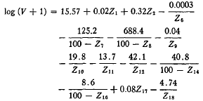
19 This general form had to be modified in several ways to handle problems peculiar to this set of data. The value one was added to all the scale scores sothat the log of these scores, the dependent variable, ranged from zero to 1.609. The reciprocal was not used for the dummy variables, Z1, to Z5. The Z's refer to the variables in Appendix B. This in effect raises or lowers the asymptote depending on the sign of the coefficients. The reciprocal form for Z17, Farm Union membership per 100 people over 25, was not used because there were a large number of zero values for this variable. For any remaining variables with any zero observations, these zeroes were replaced by 0.001 so that the reciprocal took on the value 1000. Finally, since a positive coefficient for any of the reciprocal terms implies a vastly different model than the one hypothesized, any variables with a negative effect on senators' voting behavior was entered as the reciprocal of 100 minus the variable. The following is an example of the constituency model estimated for the Area Redevelopment Act,

The constituency variables were then obtained by subtracting one from the exponential of the estimated value of each senator on each bill. These are not designed to be the “best” equations, and it is not appropriate to make any definite statements aboutthe causal effects of any one variable on Senate voting behavior. Many of the variables are quite co-linear causing additional problems in assigning significance to them. No attempt was made to purge the equations of all the statistically insignificant variables because only the estimated vote is important, not the individual coefficients. Deletion of these insignificant variables would not appreciably change these estimates.
20 Miller, Warren E. and Stokes, Donald E.,“Constituency Influence in Congress,” American Political Science Review, LVII (March, 1963), 51–53 Google Scholar.
21 Interview with Mr. William Gibbon, presently the Chairman of the Department of Political Science, Texas A&M College, College Station, Texas, March 15, 1968.
22 Jackson, John, “Some Indirect Evidences of Constituency Pressures on the Senate,” Public Policy, XVI (1967), pp. 253–270 Google Scholar.
23 Interview with Mr. James Sundquist, The Brookings Institution, Washington, D.C., March 13, 1968.
24 Interview with Mr. Sam Merrick, Office of the Mayor, Boston, Massachusetts, November, 1967. Mr. Merrick had previously handled Congressional Relations for the Labor Department.
25 Interview with Mr. James Sundquist, op. cit.
26 Key, V. O. Jr., Southern Politics (New York: Alfred A. Knopf Co., 1949), pp. 359–360 Google Scholar.
27 Huitt, Ralph K., “The Outsider in the Senate: An Alternative Role,” American Political Science Review, LV (September, 1961), 569 Google Scholar.
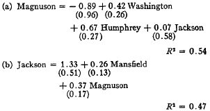
28 These senior-junior influences were examples of relationships where simultaneity was suspected. This possibility was tested in five different cases. The five cases were Magnuson and Jackson (Dem., Washington), McNamara and Hart (Dem., Michigan), Hill and Sparkman (Dem., Alabama), Schoeppel and Carlson (Rep., Kansas) and Hruska and Curtis (Rep., Nebraska). The estimations of these models were made using a two-stageleast squares procedure to test for the presence of simultaneity. In three cases, the coefficient for the effect of the junior senator on the senior senator went to zero, or very close and was not statistically significant, while the effect of the senior on the junior senator stayed very close to the same value, and was still statistically significant. Senators Magnuson and Jackson (Dem., Washington) provide an excellent example of this result. Equations (a) and (b) are the two stage least squares estimates of their models.

(Standard Errors in parentheses)
The significant point in this result is that when the appropriate two-stage procedure isused, the hypothesized influence of Jackson on Magnuson is both small and statistically insignificant. The reverse relationship, that of Magnuson on Jackson, was fairly high and statistically significant. The conclusion is that this is not a simultaneous relationship and that both senators' models can be estimated using anordinary least squares technique, with Jackson omitted from Magnuson's equation.
A minor aberration was Curtis and Hruska (Rep., Nebraska). In the two-stage estimations only the influence of Curtis on Hruska was significant. These two men came into the Senate less than two months apart, Hruska on November 8, 1954, and Curtis on January 1, 1955, so technically Hruska is the senior senator. However, both were former members of the House, Curtis for 16 years and Hruska for only 2. Thus, prior to coming to the Senate, Curtis was clearly the senior person. Consequently, the formal definitions of senior and junior senator are hypothesized to have broken down in this case.
The exception, of the five pairs, was Senators Hill and Sparkman of Alabama. Each of these two has been in the Senate a long time and is a clear anomaly among the other Southern senators as far as their voting records are concerned. For these reasons, I expected that there would be a considerable amount of discussion and interaction between these two and a breakdown of the formal senior-junior role. In spite of these factors, Hill, the senior, had a larger effect on Sparkman, the junior, than vice versa when both were estimated by a two-stage least squares method.
29 This procedure for testing a model's predictions against those of a naive model is suggested by Henri Theil. Their's models are usually trying to predict changes in an economic time series and his naive model is that there will be no change. Consequently, his statistic, called the Theil U, is the positive square root of

(where A1, is the actual change and P1, is the predicted change. The similarity between this and Equation (5) should be apparent). See Theil, Henri, Applied Economic Forecasting (Chicago: Rand McNally & Co., 1966), pp. 26–29 Google Scholar.
30 These evaluations of better and worse are based on a mean squared error criteria. This implies a quadratic loss function which means that many small errors are preferable to one large error. See ibid.
31 This interpretation of the R2 can be shown from the formula used to compute the R2 from a regression model.
where Y i is the observed value of Y and Ŷi is the predicted value of Y i from the regression model. The similarity between this and one minus Equation 5 if Y j is substituted for all Si,j should be obvious.
32 The idea of using the R2 value obtained by regressingthe actual scores against the predicted scores, which is the simple correlation between the two variables squared, was rejected for two reasons. In the first place, this comparison favors the procedure used to make the predictions. Regressing the actual scores on the predicted scores corrects for any systematic errors, such as overpredictions or underpredictions, before the comparison of the type in Equation 5 is made. In fact Theil suggests this precise procedure as one way to improve the forecasting ability of a model. Theil, op. cit., pp. 34–36. Thus the procedure used here will lead to higher values of U than the comparison of simple correlations or R2 between predicted and actual scores. The second reason for using this procedure, is that it permits a direct comparison between the errors of the postulated models and a naive model. A comparison between an R2 or a simple correlation does not provide this because both are arithmetic transformations of the errors from the two models.
33 Evans, Rowland and Novak, Robert, Lyndon B. Johnson: The Exercise of Power (New York: The New AmericanLibrary, 1966), Signet Edition, pp. 141–142, 150 Google Scholar.
- 19
- Cited by


Comments
No Comments have been published for this article.