


1. Introduction
Let
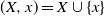
 $X = (X_1, \ldots, X_n)$
be a random vector with coordinates in a Polish space E, and let
$X = (X_1, \ldots, X_n)$
be a random vector with coordinates in a Polish space E, and let
 $f\,:\, E^n \to \mathbb{R}$
be a measurable function such that f(X), for n large, is square-integrable. For a large class of such functions f it is expected that as n grows without bound, f(X) behaves like a normal random variable. To quantify such estimates one is interested in bounding the distance between f(X) and the normal random variable
$f\,:\, E^n \to \mathbb{R}$
be a measurable function such that f(X), for n large, is square-integrable. For a large class of such functions f it is expected that as n grows without bound, f(X) behaves like a normal random variable. To quantify such estimates one is interested in bounding the distance between f(X) and the normal random variable
 $\mathcal{N} \sim N (m_f, \sigma_f^2)$
where
$\mathcal{N} \sim N (m_f, \sigma_f^2)$
where
 $m_f = \mathbb{E}[f(X)]$
and
$m_f = \mathbb{E}[f(X)]$
and
 $\sigma_f^2 = Var (f(X))$
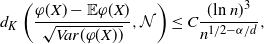
. Two such distances of interest are the Kolmogorov distance
$\sigma_f^2 = Var (f(X))$
. Two such distances of interest are the Kolmogorov distance
 \begin{align}\notag d_K(f(X), \mathcal{N}) \,{:}\,{\raise-1.5pt{=}}\, \sup_{t \in \mathbb{R}} |\mathbb{P} (f(X) \leq t) - \mathbb{P}(\mathcal{N} \leq t)|\end{align}
and the Wasserstein distance
 \begin{align}\notag d_W (f(X), \mathcal{N}) \,{:}\,{\raise-1.5pt{=}}\, \sup_{h} | \mathbb{E}[ h(f(X)) ] - \mathbb{E}[h(\mathcal{N})] |,\end{align}
where this last supremum is taken over real-valued Lipschitz functions h such that
 $|h(x) - h(y)| \leq |x - y|$
for all
$|h(x) - h(y)| \leq |x - y|$
for all
 $x, y \in \mathbb{R}$
.
$x, y \in \mathbb{R}$
.
For the case where the components of X are independent random variables, upper bounds on
 $d_W(f(X), \mathcal{N})$
were first obtained in [Reference Chatterjee2], and these were extended to
$d_W(f(X), \mathcal{N})$
were first obtained in [Reference Chatterjee2], and these were extended to
 $d_K(f(X), \mathcal{N})$
in [Reference Lachièze-Rey and Peccati14]. Both results rely on a class of difference operators that will be described in Section 2.
$d_K(f(X), \mathcal{N})$
in [Reference Lachièze-Rey and Peccati14]. Both results rely on a class of difference operators that will be described in Section 2.
Very few results address the (weakly) dependent case, and in the present work we provide estimates on
 $d_K(f(X), \mathcal{N})$
and
$d_K(f(X), \mathcal{N})$
and
 $d_W(f(X), \mathcal{N})$
when X is generated by a hidden Markov model. Such models are of interest because of their many applications in fields such as computational biology and speech recognition; see e.g. [Reference Durbin, Eddy, Krogh and Mitchison7]. Recall that a hidden Markov model (Z, X) consists of a Markov chain
$d_W(f(X), \mathcal{N})$
when X is generated by a hidden Markov model. Such models are of interest because of their many applications in fields such as computational biology and speech recognition; see e.g. [Reference Durbin, Eddy, Krogh and Mitchison7]. Recall that a hidden Markov model (Z, X) consists of a Markov chain
 $Z = (Z_1, \ldots, Z_n)$
which emits the observed variables
$Z = (Z_1, \ldots, Z_n)$
which emits the observed variables
 $X = (X_1, \ldots, X_n)$
. The possible states in Z are each associated with a distribution on the values of X. In other words the observation X is a mixture model where the choice of the mixture component for each observation depends on the component of the previous observation. The mixture components are given by the sequence Z. Note also that given Z, X is a Markov chain.
$X = (X_1, \ldots, X_n)$
. The possible states in Z are each associated with a distribution on the values of X. In other words the observation X is a mixture model where the choice of the mixture component for each observation depends on the component of the previous observation. The mixture components are given by the sequence Z. Note also that given Z, X is a Markov chain.
The content of the paper is as follows. Section 2 contains a short overview of results on normal approximation in the independent setting and introduces a simple transformation involving independent and identically distributed (i.i.d.) random variables that allows us to adapt these estimates to the hidden Markov model. Moreover, further quantitative bounds are provided for the special case when f is a Lipschitz function with respect to the Hamming distance. Applications to variants of the ones analyzed in [Reference Chatterjee2] and [Reference Lachièze-Rey and Peccati14] are developed in Sections 3 and 4, leading to an extra log-factor in the various rates obtained there. The majority of the more technical computations are carried out and presented in Section 5.
2. Main results
For a comprehensive review of Stein’s method we refer the reader to [Reference Chen, Goldstein and Shao4]. The exchangeable pairs approach was outlined in [Reference Chatterjee2]. We now recall below a few of its main points.
Let
 $W \,{:}\,{\raise-1.5pt{=}}\, f(X)$
. Originally in [Reference Chatterjee2], and then in [Reference Lachièze-Rey and Peccati14], various bounds on the distance between W and the normal distribution were obtained through a variant of Stein’s method. As is well known, Stein’s method is a way to obtain normal approximations based on the observation that the standard normal distribution
$W \,{:}\,{\raise-1.5pt{=}}\, f(X)$
. Originally in [Reference Chatterjee2], and then in [Reference Lachièze-Rey and Peccati14], various bounds on the distance between W and the normal distribution were obtained through a variant of Stein’s method. As is well known, Stein’s method is a way to obtain normal approximations based on the observation that the standard normal distribution
 $\mathcal{N}$
is the only centered and unit-variance distribution that satisfies
$\mathcal{N}$
is the only centered and unit-variance distribution that satisfies
 \begin{align}\notag \mathbb{E}\big[g^{\prime}(\mathcal{N})\big] = \mathbb{E}\big[ \mathcal{N}g(\mathcal{N})\big]\end{align}
for all absolutely continuous g with almost-everywhere (a.e.) derivative g
′ such that
 $\mathbb{E}|g^{\prime}(\mathcal{N})| < \infty$
(see [Reference Chen, Goldstein and Shao4]), and for the random variable W,
$\mathbb{E}|g^{\prime}(\mathcal{N})| < \infty$
(see [Reference Chen, Goldstein and Shao4]), and for the random variable W,
 $|\mathbb{E}[ W g(W) - g^{\prime}(W)]|$
can be thought of as a distance measuring the proximity of W to
$|\mathbb{E}[ W g(W) - g^{\prime}(W)]|$
can be thought of as a distance measuring the proximity of W to
 $\mathcal{N}$
. In particular, for the Kolmogorov distance, the solutions
$\mathcal{N}$
. In particular, for the Kolmogorov distance, the solutions
 $g_t$
to the differential equation
$g_t$
to the differential equation
 \begin{align}\notag \mathbb{P} (W \leq t) - \mathbb{P}(\mathcal{N} \leq t) = g^{\prime}_t(W) - W g_t(W)\end{align}
are absolutely continuous with a.e. derivative such that
 $\mathbb{E}\big| g^{\prime}_t(\mathcal{N})\big| < \infty$
(see [Reference Chen, Goldstein and Shao4]). Then,
$\mathbb{E}\big| g^{\prime}_t(\mathcal{N})\big| < \infty$
(see [Reference Chen, Goldstein and Shao4]). Then,
 \begin{align} d_K(W, \mathcal{N}) = \sup_{t \in \mathbb{R}}\big|\mathbb{E}\big[ g^{\prime}_t(W) - W g_t(W)\big]\big|.\end{align}
Further properties of the solutions
 $g_t$
allow for upper bounds on
$g_t$
allow for upper bounds on
 $\mathbb{E}\big[ g^{\prime}_t (W) - W g_t(W)\big]$
using difference operators associated with W that were introduced in [Reference Chatterjee2] (see [Reference Lachièze-Rey and Peccati14]). This is called the generalized perturbative approach in [Reference Chatterjee3], and we describe it next. First, we recall the perturbations used to bound the right-hand side of (1) in [Reference Chatterjee2, Reference Lachièze-Rey and Peccati14]. Let
$\mathbb{E}\big[ g^{\prime}_t (W) - W g_t(W)\big]$
using difference operators associated with W that were introduced in [Reference Chatterjee2] (see [Reference Lachièze-Rey and Peccati14]). This is called the generalized perturbative approach in [Reference Chatterjee3], and we describe it next. First, we recall the perturbations used to bound the right-hand side of (1) in [Reference Chatterjee2, Reference Lachièze-Rey and Peccati14]. Let
 $X^{\prime} = \big(X^{\prime}_1, \ldots, X^{\prime}_n\big)$
be an independent copy of X, and let
$X^{\prime} = \big(X^{\prime}_1, \ldots, X^{\prime}_n\big)$
be an independent copy of X, and let
 $W^{\prime} = f(X^{\prime})$
. Then (W, W
′) is an exchangeable pair, since it has the same joint distribution as (W
′, W). A perturbation
$W^{\prime} = f(X^{\prime})$
. Then (W, W
′) is an exchangeable pair, since it has the same joint distribution as (W
′, W). A perturbation
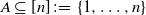
 $W^A = f^A(X) \,{:}\,{\raise-1.5pt{=}}\, f\big(X^A\big)$
of W is defined through the change
$W^A = f^A(X) \,{:}\,{\raise-1.5pt{=}}\, f\big(X^A\big)$
of W is defined through the change
 $X^A$
of X as follows:
$X^A$
of X as follows:
 \begin{align}\notag X_i^{A} =\left\{ \begin{array}{l@{\quad}l} X^{\prime}_i & \mbox{if } i \in A, \\[5pt] X_i & \mbox{if } i \notin A, \end{array}\right.\end{align}
for any
 $A \subseteq [n] \,{:}\,{\raise-1.5pt{=}}\, \{1, \ldots, n\}$
, including
$A \subseteq [n] \,{:}\,{\raise-1.5pt{=}}\, \{1, \ldots, n\}$
, including
 $A = \emptyset$
. With these definitions, still following [Reference Chatterjee2], difference operators are defined for any
$A = \emptyset$
. With these definitions, still following [Reference Chatterjee2], difference operators are defined for any
 $\emptyset \subseteq A \subseteq [n]$
and
$\emptyset \subseteq A \subseteq [n]$
and
 $i \notin A$
, as follows:
$i \notin A$
, as follows:
 \begin{align}\notag \Delta_i f^A = f\big(X^A\big) - f\Big(X^{A \cup \{i\}}\Big).\end{align}
Moreover, set
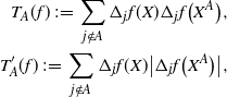 \begin{align}\notag T_A(f) \,{:}\,{\raise-1.5pt{=}}\, \sum_{j \notin A} \Delta_j f(X) \Delta_j f\big(X^A\big), \\\notag T^{\prime}_A (f) \,{:}\,{\raise-1.5pt{=}}\, \sum_{j \notin A} \Delta_j f(X) \big|\Delta_j f\big(X^A\big)\big|,\end{align}
and for
 $k_{n, A} = 1 / \Big(\begin{array}{c}n\\|A|\end{array}\Big) (n - |A|)$
, set
$k_{n, A} = 1 / \Big(\begin{array}{c}n\\|A|\end{array}\Big) (n - |A|)$
, set
 \begin{align}\notag T_n(f) \,{:}\,{\raise-1.5pt{=}}\, \sum_{\emptyset \subseteq A \subsetneq [n] } k_{n, A} T_A(f), \\\notag T^{\prime}_n(f) \,{:}\,{\raise-1.5pt{=}}\, \sum_{\emptyset \subseteq A \subsetneq [n]} k_{n, A} T^{\prime}_A (f).\end{align}
Now, for
 $W = f(X_1, \ldots, X_n)$
such that
$W = f(X_1, \ldots, X_n)$
such that
 $\mathbb{E} [W ]= 0$
,
$\mathbb{E} [W ]= 0$
,
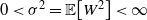
 $0 < \sigma^2 = \mathbb{E} \big[W^2\big] < \infty$
, and assuming all the expectations below are finite, [Reference Chatterjee2, Theorem 2.2] gives the bound
$0 < \sigma^2 = \mathbb{E} \big[W^2\big] < \infty$
, and assuming all the expectations below are finite, [Reference Chatterjee2, Theorem 2.2] gives the bound
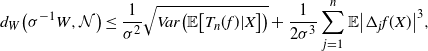 \begin{align} d_W\big(\sigma^{-1} W, \mathcal{N}\big) \leq \frac{1}{\sigma^2} \sqrt{Var \big( \mathbb{E}\big[ T_n(f) |X \big] \big) } + \frac{1}{2 \sigma^3} \sum_{j = 1}^n \mathbb{E} \big| \Delta_j f(X)\big|^3,\end{align}
while [Reference Lachièze-Rey and Peccati14, Theorem 4.2] yields
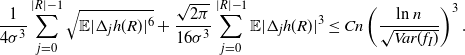
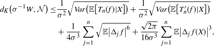 \begin{align}\notag d_K\big(\sigma^{-1} W, \mathcal{N}\big) \leq & \frac{1}{\sigma^2} \sqrt{Var\big( \mathbb{E} \big[ T_n(f) | X\big]\big)} + \frac{1}{\sigma^2} \sqrt{Var\big( \mathbb{E} \big[ T^{\prime}_n (f) | X\big]\big)} \\ & + \frac{1}{4 \sigma^3} \sum_{j = 1}^n \sqrt{\mathbb{E} \big| \Delta_j\, f\big|^6} + \frac{\sqrt{2 \pi} } {16 \sigma^3} \sum_{j = 1}^n \mathbb{E} \big|\Delta_j\, f(X)\big|^3,\end{align}
where in both cases
 $\mathcal{N}$
is now a standard normal random variable.
$\mathcal{N}$
is now a standard normal random variable.
Our main abstract result generalizes (2) and (3) to the case when X is generated by a hidden Markov model. It is as follows.
Proposition 2.1. Let
 $(Z, X)$
be a hidden Markov model with Z an aperiodic time-homogeneous and irreducible Markov chain with finite state space
$(Z, X)$
be a hidden Markov model with Z an aperiodic time-homogeneous and irreducible Markov chain with finite state space
 $\mathcal{S}$
, and X taking values in a non-empty finite
$\mathcal{S}$
, and X taking values in a non-empty finite
 $\mathcal{A}$
. Let
$\mathcal{A}$
. Let
 $W \,{:}\,{\raise-1.5pt{=}}\, f(X_1, \ldots, X_n)$
with
$W \,{:}\,{\raise-1.5pt{=}}\, f(X_1, \ldots, X_n)$
with
 $\mathbb{E}[W] = 0$
and
$\mathbb{E}[W] = 0$
and
 $0 < \sigma^2 = \mathbb{E}\big[W^2\big] < \infty$
. Then there exist a finite sequence of independent random variables
$0 < \sigma^2 = \mathbb{E}\big[W^2\big] < \infty$
. Then there exist a finite sequence of independent random variables
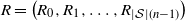 $R = \big(R_0, R_1, \ldots, R_{|\mathcal{S}|(n-1)}\big)$
, with
$R = \big(R_0, R_1, \ldots, R_{|\mathcal{S}|(n-1)}\big)$
, with
 $R_i$
taking values in
$R_i$
taking values in
 $\mathcal{S} \times \mathcal{A}$
for
$\mathcal{S} \times \mathcal{A}$
for
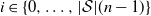
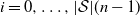 $i = 0, \ldots, |\mathcal{S}|(n-1)$
, and a measurable function
$i = 0, \ldots, |\mathcal{S}|(n-1)$
, and a measurable function
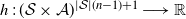 $h\,:\, (\mathcal{S} \times \mathcal{A})^{|\mathcal{S}|(n-1)+1} \longrightarrow \mathbb{R}$
such that
$h\,:\, (\mathcal{S} \times \mathcal{A})^{|\mathcal{S}|(n-1)+1} \longrightarrow \mathbb{R}$
such that
 $h\big(R_0, \ldots, R_{|\mathcal{S}| (n-1)} \big)$
and
$h\big(R_0, \ldots, R_{|\mathcal{S}| (n-1)} \big)$
and
 $f(X_1, \ldots, X_n)$
are identically distributed. Therefore,
$f(X_1, \ldots, X_n)$
are identically distributed. Therefore,
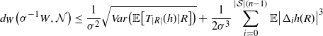 \begin{align} d_W\big(\sigma^{-1} W, \mathcal{N} \big) \leq \frac{1}{\sigma^2} \sqrt{Var\big( \mathbb{E}\big[T_{|R|}(h) |R \big] \big)} + \frac{1}{2 \sigma^3} \sum_{i = 0}^{|\mathcal{S}|(n-1)} \mathbb{E}\big| \Delta_i h(R)\big|^3\end{align}
and
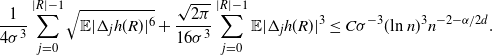
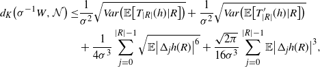 \begin{align}\notag d_K \big(\sigma^{-1} W, \mathcal{N}\big) \leq & \frac{1}{\sigma^2} \sqrt{Var\big( \mathbb{E} \big[ T_{|R|}(h) | R\big]\big)} + \frac{1}{\sigma^2} \sqrt{Var\big( \mathbb{E} \big[ T^{\prime}_{|R|} (h) | R\big]\big)} \\ & + \frac{1}{4 \sigma^3} \sum_{j = 0}^{|R| - 1} \sqrt{\mathbb{E} \big| \Delta_j h(R)\big|^6} + \frac{\sqrt{2 \pi} } {16 \sigma^3} \sum_{j = 0}^{|R| - 1} \mathbb{E} \big|\Delta_j h(R)\big|^3,\end{align}
where
 $\mathcal{N}$
is a standard normal random variable.
$\mathcal{N}$
is a standard normal random variable.
At first glance the above results might appear to be simple corollaries to (2) and (3). Indeed, as is well known, every Markov chain (in a Polish space) admits a representation via i.i.d. random variables
 $U_1, \ldots, U_n$
, uniformly distributed on (0, 1), and the inverse distribution function. Therefore,
$U_1, \ldots, U_n$
, uniformly distributed on (0, 1), and the inverse distribution function. Therefore,
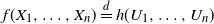 $f(X_1, \ldots, X_n) \overset{d}{=} h(U_1, \ldots, U_n)$
, for some function h, where, as usual,
$f(X_1, \ldots, X_n) \overset{d}{=} h(U_1, \ldots, U_n)$
, for some function h, where, as usual,
 $\overset{d}{=}$
indicates equality in distribution. However, providing quantitative estimates for
$\overset{d}{=}$
indicates equality in distribution. However, providing quantitative estimates for
 $\mathbb{E} |\Delta_j h(U_1, \ldots, U_n)|$
via f seems to be out of reach, since passing from f to h involves the ‘unknown’ inverse distribution function. For this reason, we develop for our analysis a more amenable, although more restrictive, choice of i.i.d. random variables, which is described intuitively in the next paragraph and then again in greater detail in Section 2.1.
$\mathbb{E} |\Delta_j h(U_1, \ldots, U_n)|$
via f seems to be out of reach, since passing from f to h involves the ‘unknown’ inverse distribution function. For this reason, we develop for our analysis a more amenable, although more restrictive, choice of i.i.d. random variables, which is described intuitively in the next paragraph and then again in greater detail in Section 2.1.
Consider
 $R = \big(R_0, \ldots, R_{|\mathcal{S}|(n-1)}\big)$
as stacks of independent random variables on the
$R = \big(R_0, \ldots, R_{|\mathcal{S}|(n-1)}\big)$
as stacks of independent random variables on the
 $|\mathcal{S}|$
possible states of the hidden chain that determine the next step in the process, with
$|\mathcal{S}|$
possible states of the hidden chain that determine the next step in the process, with
 $R_0$
specifying the initial state. Each
$R_0$
specifying the initial state. Each
 $R_i$
takes values in
$R_i$
takes values in
 $\mathcal{S} \times \mathcal{A}$
and is distributed according to the transition probability from the present hidden state. Then, one has
$\mathcal{S} \times \mathcal{A}$
and is distributed according to the transition probability from the present hidden state. Then, one has
 $f\big(X_1, \ldots , X_n\big) \overset{d}{=} h \big(R_0, \ldots , R_{|\mathcal{S}|(n-1)}\big)$
, for
$f\big(X_1, \ldots , X_n\big) \overset{d}{=} h \big(R_0, \ldots , R_{|\mathcal{S}|(n-1)}\big)$
, for
 $h = f \circ \gamma$
, where the function
$h = f \circ \gamma$
, where the function
 $\gamma$
translates between R and X. This construction is carried out in more detail in the next section. Further note that when
$\gamma$
translates between R and X. This construction is carried out in more detail in the next section. Further note that when
 $(X_i)_{i \geq 1}$
is a sequence of independent random variables, the hidden chain in the model consists of a single state, and then the function
$(X_i)_{i \geq 1}$
is a sequence of independent random variables, the hidden chain in the model consists of a single state, and then the function
 $\gamma$
is the identity function and so
$\gamma$
is the identity function and so
 $h = f$
.
$h = f$
.
In order for Proposition 2.1 to be meaningful, a further quantitative study of the terms in the upper bounds is necessary. It turns out that the variance terms determine the order of decay; see Remark 5.2. Nevertheless, we obtain additional quantitative estimates for all the terms involved; the proofs are presented in Section 5.
Proposition 2.2. With the notation as above, let f be Lipschitz with respect to the Hamming distance, i.e., let
 \begin{equation*}|f(x) - f(y)| \leq c \sum_{i = 1}^n \mathbf{1}_{x_i \neq y_i}\end{equation*}
for every
 $x, y \in \mathcal{A}^n$
and where
$x, y \in \mathcal{A}^n$
and where
 $c > 0$
. Then, for any
$c > 0$
. Then, for any
 $r > 0$
,
$r > 0$
,
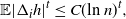
 \begin{align}\notag \mathbb{E} |\Delta_i h(R)|^r \leq & C_1 (\text{ln}\ n)^r, \\\notag \mathbb{E} |h(R) - \mathbb{E}[h(R)]|^r \leq & C_2 n^{r/2} (\text{ln}\ n)^r,\end{align}
for n large enough and
 $C_1, C_2 > 0$
depending on r and the parameters of the model.
$C_1, C_2 > 0$
depending on r and the parameters of the model.
Let R
′ and R
′′ be independent copies of R, and let
 $\widetilde{\mathbf{R}}$
be the random set of recombinations of R, R
′, and R
′′. The set
$\widetilde{\mathbf{R}}$
be the random set of recombinations of R, R
′, and R
′′. The set
 $\widetilde{\mathbf{R}}$
consists of
$\widetilde{\mathbf{R}}$
consists of
 $3^{|R|}$
random vectors of size
$3^{|R|}$
random vectors of size
 $|R|$
:
$|R|$
:
 \begin{align}\notag \widetilde{\mathbf{R}} \,{:}\,{\raise-1.5pt{=}}\, \left\{ Z = \big(Z_0, \ldots, Z_{|R|-1} \big)\,:\, Z_i \in \big\{ R_i, R^{\prime}_i, R^{\prime\prime}_i \big\} \right\}.\end{align}
Let
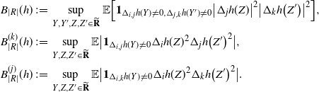 \begin{align}\begin{split} B_{|R|}(h) \,{:}\,{\raise-1.5pt{=}}\, & \sup_{Y, Y^{\prime}, Z, Z^{\prime} \in \widetilde{\mathbf{R}}} \mathbb{E} \Big[\mathbf{1}_{\Delta_{i,j} h(Y) \neq 0, \Delta_{j,k} h(Y^{\prime}) \neq 0} \big|\Delta_j h(Z)\big|^2 \big|\Delta_k h\big(Z^{\prime}\big)\big|^2\Big],\\ B_{|R|}^{(k)}(h) \,{:}\,{\raise-1.5pt{=}}\, & \sup_{Y, Z, Z^{\prime} \in \widetilde{\mathbf{R}} } \mathbb{E} \big| \mathbf{1}_{\Delta_{i,j} h(Y) \neq 0} \Delta_i h(Z)^2 \Delta_j h\big(Z^{\prime}\big)^2\big|, \\ B_{|R|}^{(j)} (h) \,{:}\,{\raise-1.5pt{=}}\, & \sup_{Y, Z, Z^{\prime} \in \widetilde{\mathbf{R}}} \mathbb{E} \big| \mathbf{1}_{\Delta_{i,k} h(Y) \neq 0} \Delta_i h(Z)^2 \Delta_k h\big(Z^{\prime}\big)^2\big|.\end{split}\end{align}
Then the following general bound for the variance terms holds.
Proposition 2.3. With the notation as above and for
 $U = T_{|R|}(h)$
or
$U = T_{|R|}(h)$
or
 $U = T^{\prime}_{|R|}(h)$
, we have
$U = T^{\prime}_{|R|}(h)$
, we have
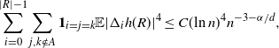
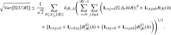 \begin{align}\notag & \sqrt{Var\big(\mathbb{E}[U|R]\big)} \leq \frac{1}{\sqrt{2}} \sum_{\emptyset \subseteq A \subsetneq[|R|]} k_{|R|, A} \Bigg( \sum_{i = 0}^{|R| -1} \sum_{j, k \notin A}\bigg( \mathbf{1}_{i = j = k} \mathbb{E} |\Delta_i h(R)|^4 + \mathbf{1}_{i \neq j \neq k} B_{|R|}(h) \\\notag & \quad \quad \quad \quad \quad \quad \quad \quad + \big(\mathbf{1}_{i \neq j = k} + \mathbf{1}_{i = k \neq j} \big) B_{|R|}^{(k)}(h) + \big(\mathbf{1}_{i \neq j = k} + \mathbf{1}_{i = j \neq k} \big) B_{|R|}^{(j)}(h) \bigg) \Bigg)^{1/2},\end{align}
where
 $[|R|] \,{:}\,{\raise-1.5pt{=}}\, \{1, \ldots, |R| \}$
.
$[|R|] \,{:}\,{\raise-1.5pt{=}}\, \{1, \ldots, |R| \}$
.
Note that in Proposition 2.3, the underlying function f is not assumed to be Lipschitz. Moreover, the function h is not symmetric, and therefore the expression above cannot be simplified further, in contrast to the similar results in [Reference Lachièze-Rey and Peccati14]. The proofs of Propositions 2.2 and 2.3 are technical and are delayed to Sections 5.1 and 5.2 respectively.
2.1. Additional details on the construction of R
Let (Z, X) be a hidden Markov model with Z an aperiodic time-homogeneous and irreducible Markov chain on a finite state space
 $\mathcal{S}$
, and with X taking values in an alphabet
$\mathcal{S}$
, and with X taking values in an alphabet
 $\mathcal{A}$
. Let P be the transition matrix of the hidden chain, and let Q be the
$\mathcal{A}$
. Let P be the transition matrix of the hidden chain, and let Q be the
 $|\mathcal{S}| \times |\mathcal{A}|$
probability matrix for the observations; i.e.,
$|\mathcal{S}| \times |\mathcal{A}|$
probability matrix for the observations; i.e.,
 $Q_{ij}$
is the probability of seeing output j if the latent chain is in state i. Let the initial distribution of the hidden chain be
$Q_{ij}$
is the probability of seeing output j if the latent chain is in state i. Let the initial distribution of the hidden chain be
 $\mu$
. Then
$\mu$
. Then
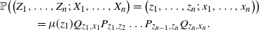 \begin{align}\notag & \mathbb{P} \big( \big(Z_1, \ldots, Z_n;\, X_1, \ldots, X_n\big) = \big(z_1, \ldots, z_n;\, x_1, \ldots, x_n\big) \big) \\\notag & \quad \quad \quad = \mu(z_1) Q_{z_1, x_1} P_{z_1, z_2} \ldots P_{z_{n-1}, z_n} Q_{z_n, x_n}.\end{align}
Next we introduce a sequence of independent random variables
 $R_0, \ldots, R_{|\mathcal{S}|(n-1)}$
taking values in
$R_0, \ldots, R_{|\mathcal{S}|(n-1)}$
taking values in
 $\mathcal{S} \times \mathcal{A}$
and a function
$\mathcal{S} \times \mathcal{A}$
and a function
 $\gamma$
such that
$\gamma$
such that
 $\gamma\big(R_0, \ldots, R_{|\mathcal{S}| (n-1) }\big) = \big(Z_1, \ldots, Z_n;\, X_1, \ldots , X_n\big)$
. For any
$\gamma\big(R_0, \ldots, R_{|\mathcal{S}| (n-1) }\big) = \big(Z_1, \ldots, Z_n;\, X_1, \ldots , X_n\big)$
. For any
 $s, s^{\prime} \in \mathcal{S}$
,
$s, s^{\prime} \in \mathcal{S}$
,
 $x \in \mathcal{A}$
, and
$x \in \mathcal{A}$
, and
 $i \in \{0, \ldots, n-1\}$
, let
$i \in \{0, \ldots, n-1\}$
, let
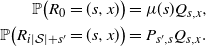 \begin{align}\notag \mathbb{P}\big(R_0 = (s, x) \big) & = \mu(s) Q_{s, x}, \\\notag \mathbb{P} \big(R_{i |\mathcal{S}| + s^{\prime}} = (s, x) \big) & = P_{s^{\prime} , s} Q_{s, x}.\end{align}
The random variables
 $R_i$
are well defined since
$R_i$
are well defined since
 $\sum_x Q_{s, x} = 1$
for any
$\sum_x Q_{s, x} = 1$
for any
 $s \in \mathcal{S}$
and
$s \in \mathcal{S}$
and
 $\sum_s P_{s^{\prime}, s} = \sum_s \mu(s) = 1$
for any
$\sum_s P_{s^{\prime}, s} = \sum_s \mu(s) = 1$
for any
 $s^{\prime} \in \mathcal{S}$
. One can think of the variables
$s^{\prime} \in \mathcal{S}$
. One can think of the variables
 $R_i$
as a set of instructions indicating where the hidden Markov model goes next. The function
$R_i$
as a set of instructions indicating where the hidden Markov model goes next. The function
 $\gamma$
reconstructs the realization
$\gamma$
reconstructs the realization
 $(Z_i, X_i)_{i \geq 1}$
sequentially from the sequence
$(Z_i, X_i)_{i \geq 1}$
sequentially from the sequence
 $(R_i)_{i \geq 0}$
. In particular,
$(R_i)_{i \geq 0}$
. In particular,
 $\gamma$
captures the following relations:
$\gamma$
captures the following relations:
 \begin{align}\notag \big(Z_1, X_1\big) & = R_0, \\\notag \big(Z_{i+1}, X_{i+1}\big) & = R_{i |\mathcal{S}| + s} \quad \mbox{ if } Z_i = s \mbox { for } i \geq 1.\end{align}
One can also think of the sequence
 $(R_i)_{i \geq 0}$
as
$(R_i)_{i \geq 0}$
as
 $|\mathcal{S}|$
stacks of random variables on the
$|\mathcal{S}|$
stacks of random variables on the
 $|\mathcal{S}|$
possible states of the latent Markov chain, and the values being rules for the next step in the model. Note that only one variable on the ith level of the stack will be used to determine the
$|\mathcal{S}|$
possible states of the latent Markov chain, and the values being rules for the next step in the model. Note that only one variable on the ith level of the stack will be used to determine the
 $(i+1)$
th hidden and observed pair. Furthermore, the distribution of the random variables
$(i+1)$
th hidden and observed pair. Furthermore, the distribution of the random variables
 $R_i$
for
$R_i$
for
 $i \geq 1$
encodes the transition and output probabilities in the P and Q matrices of the original model.
$i \geq 1$
encodes the transition and output probabilities in the P and Q matrices of the original model.
Thus one can write
 $f\big(X_1, \ldots, X_n\big) = h\big(R_0, \ldots , R_{|\mathcal{S}| (n-1) }\big)$
, for
$f\big(X_1, \ldots, X_n\big) = h\big(R_0, \ldots , R_{|\mathcal{S}| (n-1) }\big)$
, for
 $h \,{:}\,{\raise-1.5pt{=}}\, f \circ \gamma$
, where the function
$h \,{:}\,{\raise-1.5pt{=}}\, f \circ \gamma$
, where the function
 $\gamma$
does the translation from
$\gamma$
does the translation from
 $(R_i)_{i \geq 0}$
to
$(R_i)_{i \geq 0}$
to
 $\big(Z_i, X_i\big)_{i \geq 1}$
as described above.
$\big(Z_i, X_i\big)_{i \geq 1}$
as described above.
Let
 $R^{\prime} = \big(R^{\prime}_0, \ldots, R_{|\mathcal{S}| (n-1)}^{\prime}\big)$
be an independent copy of R. Let
$R^{\prime} = \big(R^{\prime}_0, \ldots, R_{|\mathcal{S}| (n-1)}^{\prime}\big)$
be an independent copy of R. Let
 $A \subseteq \{0, 1, \ldots, |\mathcal{S}|(n-1)\}$
, and let the change
$A \subseteq \{0, 1, \ldots, |\mathcal{S}|(n-1)\}$
, and let the change
 $R^A$
of R be defined as follows:
$R^A$
of R be defined as follows:
 \begin{align} R_i^A = \left\{ \begin{array}{r@{\quad}l} R^{\prime}_i & \mbox { if } i \in A, \\[4pt] R_i & \mbox{ if } i \notin A, \end{array}\right.\end{align}
where, as before, when
 $A = \{j\}$
we write
$A = \{j\}$
we write
 $R^j$
instead of
$R^j$
instead of
 $R^{\{j\}}$
.
$R^{\{j\}}$
.
Recall that the ‘discrete derivative’ of h with a perturbation A is
 \begin{align}\notag \Delta_i h^A = h\big(R^A\big) - h \big(R^{A \cup \{i\}}\big).\end{align}
Then (4) and (5) follow from (2) and (3), respectively, since when (Z, X) is a hidden Markov model one writes
 \begin{align}\notag W = f\big(X_1, \ldots, X_n\big) \overset{d}{=} h \big(R_0, \ldots, R_{|\mathcal{S}|(n-1)}\big),\end{align}
where the sequence
 $(R_i)_{i \geq 0}$
is a sequence of independent random variables.
$(R_i)_{i \geq 0}$
is a sequence of independent random variables.
Remark 2.1. (i) The idea of using stacks of independent random variables to represent a hidden Markov model is somewhat reminiscent of Wilson’s cycle popping algorithm for generating a random directed spanning tree; see [Reference Wilson17]. The algorithm has also been related to loop-erased random walks in [Reference Gorodezky and Pak9].
(ii) If S consists of a single state, making the hidden chain redundant, there is a single stack of instructions. This corresponds to the independent setting of [Reference Chatterjee2] and [Reference Lachièze-Rey and Peccati14], and then
 $\gamma$
is just the identity function.
$\gamma$
is just the identity function.
(iii) The same approach, via the use of instructions, is also applicable when
 $\mathcal{A}$
and
$\mathcal{A}$
and
 $\mathcal{S}$
are infinite countable. The
$\mathcal{S}$
are infinite countable. The
 $Q_{s,x}$
no longer form a finite matrix, but the same definition holds as long as
$Q_{s,x}$
no longer form a finite matrix, but the same definition holds as long as
 $\sum_{x \in \mathcal{A}} Q_{s,x} = 1$
for all
$\sum_{x \in \mathcal{A}} Q_{s,x} = 1$
for all
 $s \in \mathcal{S}$
. We need a countably infinite number of independent instructions to encode
$s \in \mathcal{S}$
. We need a countably infinite number of independent instructions to encode
 $(Z_i, X_i)_{1 \leq i \leq n}$
. In particular, let
$(Z_i, X_i)_{1 \leq i \leq n}$
. In particular, let
 $R_0$
and
$R_0$
and
 $\big(R_{i, s}\big)_{1 \leq i \leq n, s \in \mathcal{S}}$
be such that
$\big(R_{i, s}\big)_{1 \leq i \leq n, s \in \mathcal{S}}$
be such that
 \begin{align}\notag \mathbb{P}\big(R_0 = (s,x) \big) = \mu(s) Q_{s,x}, \\\notag \mathbb{P}\big(R_{i,s^{\prime}} = (s, x)\big) = P_{s^{\prime}, s} Q_{s,x}.\end{align}
Then the function
 $\gamma$
reconstructs
$\gamma$
reconstructs
 $\big(Z_i, X_i\big)_{1 \leq i \leq n}$
from
$\big(Z_i, X_i\big)_{1 \leq i \leq n}$
from
 $R_0$
and
$R_0$
and
 $\big(R_{i,s}\big)_{1 \leq i \leq n, s \in \mathcal{S}}$
via
$\big(R_{i,s}\big)_{1 \leq i \leq n, s \in \mathcal{S}}$
via
 \begin{align}\notag \big(Z_1, X_1\big) & = R_0, \\\notag \big(Z_{i+1}, X_{i+1} \big) & = R_{i, s} \quad \mbox{ if } Z_i = s \mbox { for } i \geq 1.\end{align}
(iv) It is possible to obtain bounds on the various terms involved in Proposition 2.2 and Proposition 2.3 in the case when
 $|\mathcal{S}|$
is a function of n. Assuming that there exists a general deterministic upper bound
$|\mathcal{S}|$
is a function of n. Assuming that there exists a general deterministic upper bound
 $g_r(n)$
on
$g_r(n)$
on
 $\mathbb{E} |\Delta_i h|^r$
, one can bound the non-variance terms in Proposition 2.2 by
$\mathbb{E} |\Delta_i h|^r$
, one can bound the non-variance terms in Proposition 2.2 by
 $C |\mathcal{S}| \left(\sqrt{ g_6(n) } + g_3(n) \right) /\sigma^3 $
. The variance terms, using Proposition 2.3, will then be bounded by
$C |\mathcal{S}| \left(\sqrt{ g_6(n) } + g_3(n) \right) /\sigma^3 $
. The variance terms, using Proposition 2.3, will then be bounded by
 $C \sqrt{ |\mathcal{S}| g_4(n) + |\mathcal{S}|^3 ( A ) } /\sigma^2$
, where A is a complicated expression that depends on the particular problem as well as on
$C \sqrt{ |\mathcal{S}| g_4(n) + |\mathcal{S}|^3 ( A ) } /\sigma^2$
, where A is a complicated expression that depends on the particular problem as well as on
 $\mathbb{E}|\Delta_i h|^r$
and
$\mathbb{E}|\Delta_i h|^r$
and
 $|\mathcal{S}|$
.
$|\mathcal{S}|$
.
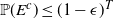
The next crucial part in the analysis is the key result we use everywhere: if a change in an instruction propagates X levels (a random variable), then
 $\mathbb{P} (X > K) \leq (1 - \epsilon)^K$
, for some absolute
$\mathbb{P} (X > K) \leq (1 - \epsilon)^K$
, for some absolute
 $0 < \epsilon < 1$
. If
$0 < \epsilon < 1$
. If
 $|\mathcal{S}|$
is finite, this holds under some standard assumptions on the model. If
$|\mathcal{S}|$
is finite, this holds under some standard assumptions on the model. If
 $|\mathcal{S}|$
grows with n, then under some minor additional restrictions in the hidden Markov model, we have
$|\mathcal{S}|$
grows with n, then under some minor additional restrictions in the hidden Markov model, we have
 $\mathbb{P}(X > K) \leq (1 - 1/|\mathcal{S}|)^K$
. Then K can be chosen to be at most a small power of n (we take
$\mathbb{P}(X > K) \leq (1 - 1/|\mathcal{S}|)^K$
. Then K can be chosen to be at most a small power of n (we take
 $K = \text{ln}\ n$
in the finite case, which explains the logarithmic factors in our bounds). For meaningful bounds,
$K = \text{ln}\ n$
in the finite case, which explains the logarithmic factors in our bounds). For meaningful bounds,
 $|\mathcal{S}|$
could grow at most like
$|\mathcal{S}|$
could grow at most like
 $\text{ln}\ n$
. However, much more fine-tuning is necessary in the actual proof.
$\text{ln}\ n$
. However, much more fine-tuning is necessary in the actual proof.
For some recent results (different from ours) on normal approximation for functions of general Markov chains we refer the reader to [Reference Chen, Shao and Xu5].
3. Covering process
Although our framework was initially motivated by [Reference Houdré and Kerchev11] and the problem of finding a normal approximation result for the length of the longest common subsequences in dependent random words, some applications to stochastic geometry are presented below. Our methodology can be applied to other related settings, in particular to the variant of the occupancy problem introduced in the recent article [Reference Grabchak, Kelbert and Paris10] (see Remark 4.1).
Let
 $(K, \mathcal{K})$
be the space of compact subsets of
$(K, \mathcal{K})$
be the space of compact subsets of
 $\mathbb{R}^d$
, endowed with the hit-and-miss topology. Let
$\mathbb{R}^d$
, endowed with the hit-and-miss topology. Let
 $E_n$
be a cube of volume n, and let
$E_n$
be a cube of volume n, and let
 $C_1, \ldots, C_n$
be random variables in
$C_1, \ldots, C_n$
be random variables in
 $E_n$
, called germs. In the i.i.d. setting of [Reference Lachièze-Rey and Peccati14], each
$E_n$
, called germs. In the i.i.d. setting of [Reference Lachièze-Rey and Peccati14], each
 $C_i$
is sampled uniformly and independently in
$C_i$
is sampled uniformly and independently in
 $E_n$
; i.e., if
$E_n$
; i.e., if
 $T \subset E_n$
with measure
$T \subset E_n$
with measure
 $|T|$
, then
$|T|$
, then
 \begin{align}\notag \mathbb{P}(C_i \in T) = \frac{|T|}{n},\end{align}
for all
 $i \in \{1, \ldots, n\}$
.
$i \in \{1, \ldots, n\}$
.
Here, we consider
 $C_1, \ldots, C_n$
, generated by a hidden Markov model in the following way. Let
$C_1, \ldots, C_n$
, generated by a hidden Markov model in the following way. Let
 $Z_1, \ldots, Z_n$
be an aperiodic irreducible Markov chain on a finite state space
$Z_1, \ldots, Z_n$
be an aperiodic irreducible Markov chain on a finite state space
 $\mathcal{S}$
. Each
$\mathcal{S}$
. Each
 $s \in \mathcal{S}$
is associated with a measure
$s \in \mathcal{S}$
is associated with a measure
 $m_s$
on
$m_s$
on
 $E_n$
. Then for each measurable
$E_n$
. Then for each measurable
 $T \subseteq E_n$
,
$T \subseteq E_n$
,
 \begin{align}\notag \mathbb{P} \big(C_i \in T | Z_i = s\big) = m_s(T).\end{align}
Assume that there are constants
 $0 < c_m \leq c_M$
such that for any
$0 < c_m \leq c_M$
such that for any
 $s \in \mathcal{S}$
and measurable
$s \in \mathcal{S}$
and measurable
 $T \subseteq E_n$
,
$T \subseteq E_n$
,
 \begin{align}\notag \frac{c_m |T|}{n} \leq m_s(T) \leq \frac{c_M |T|}{n}.\end{align}
Note that
 $c_m = c_M = 1$
recovers the setting of [Reference Lachièze-Rey and Peccati14].
$c_m = c_M = 1$
recovers the setting of [Reference Lachièze-Rey and Peccati14].
Let
 $K_1, \ldots, K_n$
be compact sets (grains) with
$K_1, \ldots, K_n$
be compact sets (grains) with
 $Vol (K_i) \in (V_1, V_2)$
(absolute constants) for
$Vol (K_i) \in (V_1, V_2)$
(absolute constants) for
 $i = 1,\ldots, n$
. Let
$i = 1,\ldots, n$
. Let
 $X_i = C_i + K_i$
for
$X_i = C_i + K_i$
for
 $i = 1, \ldots, n$
be the germ–grain process. Consider the closed set formed by the union of the germs translated by the grains
$i = 1, \ldots, n$
be the germ–grain process. Consider the closed set formed by the union of the germs translated by the grains
 \begin{align}\notag F_n = \left( \bigcup_{k =1}^n X_K\right) \cap E_n.\end{align}
We are interested in the volume covered by
 $F_n$
,
$F_n$
,
 \begin{align}\notag f_V\big(X_1, \ldots, X_n\big) = Vol(F_n),\end{align}
and the number of isolated grains,
 \begin{align}\notag f_I\big(X_1, \ldots, X_n\big) = \# \big\{ k \,:\, X_k \cap X_j \cap E_n = \emptyset, k \neq j \big\}.\end{align}
Theorem 3.1. Let
 $\mathcal{N}$
be a standard normal random variable. Then, for all
$\mathcal{N}$
be a standard normal random variable. Then, for all
 $n \in \mathbb{N}$
,
$n \in \mathbb{N}$
,
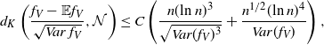 \begin{align} d_K\left(\frac{f_V - \mathbb{E} f_V}{\sqrt{Var\, f_V}} , \mathcal{N} \right) \leq C \left( \frac{ n(\text{ln}\ n)^3} {\sqrt{Var(f_V)^3}} + \frac{ n^{1/2} (\text{ln}\ n)^4}{ Var(f_V)} \right), \end{align}
 \begin{align} d_K\left(\frac{f_I - \mathbb{E} f_I}{\sqrt{Var\, f_I}} , \mathcal{N} \right) \leq C \left( \frac{ n(\text{ln}\ n)^3} {\sqrt{Var(f_I)^3}} + \frac{n^{1/2} (\text{ln}\ n)^4} {Var(f_I)}\right), \end{align}
for some constant
 $C > 0$
independent of n.
$C > 0$
independent of n.
The study of the order of growth of
 $Var f_I$
and
$Var f_I$
and
 $Var f_V$
is not really part of the scope of the present paper. In the independent case, there are constants
$Var f_V$
is not really part of the scope of the present paper. In the independent case, there are constants
 $0 < c_V \leq C_V$
such that
$0 < c_V \leq C_V$
such that
 $c_V n \leq Var f_V \leq C_V n$
and
$c_V n \leq Var f_V \leq C_V n$
and
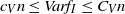 $c_V n \leq Var f_I \leq C_V n $
for n sufficiently large (see [Reference Kendall and Molchanov13, Theorem 4.4]). In our dependent setting, a variance lower bound of order n will thus provide a rate of order
$c_V n \leq Var f_I \leq C_V n $
for n sufficiently large (see [Reference Kendall and Molchanov13, Theorem 4.4]). In our dependent setting, a variance lower bound of order n will thus provide a rate of order
 $(\log n)^4/\sqrt{n}$
.
$(\log n)^4/\sqrt{n}$
.
The proofs of the normal approximations for
 $f_V$
and
$f_V$
and
 $f_I$
are carried out in Sections 3.1 and 3.2. Many of the more technical computations are carried out in Section 5.
$f_I$
are carried out in Sections 3.1 and 3.2. Many of the more technical computations are carried out in Section 5.
3.1. Normal approximation for
 $\textbf{\textit{f}}_{\textbf{\textit{V}}}$

Write
 $f_V\big(X_1, \ldots, X_n\big) = h\big(R_0, \ldots, R_{|\mathcal{S}|(n-1)}\big)$
for a set of instructions R defined as in Section 2.1. The volume of each grain is bounded by
$f_V\big(X_1, \ldots, X_n\big) = h\big(R_0, \ldots, R_{|\mathcal{S}|(n-1)}\big)$
for a set of instructions R defined as in Section 2.1. The volume of each grain is bounded by
 $V_2$
, so
$V_2$
, so
 $f_V$
is Lipschitz with respect to the Hamming distance, with constant
$f_V$
is Lipschitz with respect to the Hamming distance, with constant
 $V_2$
. Proposition 2.1 holds, and from Proposition 2.2, the non-variance terms in the bounds in Proposition 2.1 are bounded by
$V_2$
. Proposition 2.1 holds, and from Proposition 2.2, the non-variance terms in the bounds in Proposition 2.1 are bounded by
 $C (\text{ln}\ n)^3 / \sqrt{n}$
. Here and below, C is a constant, independent of n, which can vary from line to line. Indeed, for instance,
$C (\text{ln}\ n)^3 / \sqrt{n}$
. Here and below, C is a constant, independent of n, which can vary from line to line. Indeed, for instance,
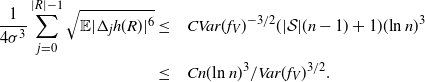 \begin{align}\notag \frac{1}{4 \sigma^3} \sum_{j = 0}^{|R| - 1} \sqrt{ \mathbb{E} |\Delta_j h(R)|^6} \leq & \quad C Var(f_V)^{-3/2} (|\mathcal{S}|(n-1) + 1) (\text{ln}\ n )^3 \\ \leq & \quad C n(\text{ln}\ n)^3 / Var(f_V)^{3/2}.\end{align}
To analyze the bound on the variance terms given by Proposition 2.3, first note that
 \begin{align}\notag \sum_{i = 0}^{|R| -1} \sum_{j, k \notin A} \mathbf{1}_{i = j = k} \mathbb{E} | \Delta_i h(R)|^4 \leq Cn (\text{ln}\ n)^4,\end{align}
using Proposition 2.2. The other terms are bounded as follows.
Proposition 3.1. Let
 $A \subsetneq [ | R | ] $
, and let
$A \subsetneq [ | R | ] $
, and let
 $B_{|R|}(h)$
,
$B_{|R|}(h)$
,
 $B_{|R|}^k(h)$
, and
$B_{|R|}^k(h)$
, and
 $B_{|R|}^j(h)$
be as in (6). Then
$B_{|R|}^j(h)$
be as in (6). Then
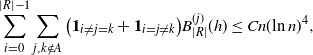
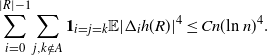
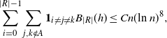 \begin{align} \sum_{i = 0}^{|R| -1} & \sum_{j, k \notin A} \mathbf{1}_{i \neq j \neq k} B_{|R|}(h) \leq Cn (\text{ln}\ n)^8, \qquad\qquad\end{align}
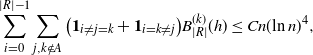 \begin{align}\sum_{i = 0}^{|R| -1} & \sum_{j, k \notin A} \big(\mathbf{1}_{i \neq j = k} + \mathbf{1}_{i = k \neq j} \big) B_{|R|}^{(k)}(h) \leq Cn (\text{ln}\ n)^4, \end{align}
 \begin{align} \sum_{i = 0}^{|R| -1} & \sum_{j, k \notin A} \big(\mathbf{1}_{i \neq j = k} + \mathbf{1}_{i = j \neq k} \big) B_{|R|}^{(j)}(h) \leq Cn (\text{ln}\ n)^4, \end{align}
for some constant
 $C > 0$
that does not depend on n.
$C > 0$
that does not depend on n.
Proof. See Section 5.3 for the proof of the first bound. The others follow similarly.
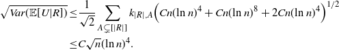
The bound on the variance terms in Proposition 2.3 becomes
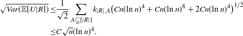 \begin{align}\notag \sqrt{Var(\mathbb{E}[U|R])} \leq & \frac{1}{\sqrt{2}} \sum_{A \subsetneq[|R|]} k_{|R|, A} \big( C n (\text{ln}\ n)^4 + Cn (\text{ln}\ n)^8 + 2 C n (\text{ln}\ n)^4 \big)^{1/2}\\ \leq & C \sqrt{n} (\text{ln}\ n)^4.\end{align}
3.2. Normal approximation for
$\textbf{\textit{f}}_{\textbf{\textit{I}}}$

The proof of (9) is more involved since the function
 $f_I$
is not Lipschitz. Abusing notation, write
$f_I$
is not Lipschitz. Abusing notation, write
 $f_I\big(X_1, \ldots, X_n\big) = h\big(R_0, \ldots, R_{|\mathcal{S}|(n-1)}\big)$
for a set of instructions R as in Section 2.1. Proposition 2.1 holds, and, as in our analysis for
$f_I\big(X_1, \ldots, X_n\big) = h\big(R_0, \ldots, R_{|\mathcal{S}|(n-1)}\big)$
for a set of instructions R as in Section 2.1. Proposition 2.1 holds, and, as in our analysis for
 $f_V$
, we proceed by estimating the non-variance terms in the bounds. The following holds.
$f_V$
, we proceed by estimating the non-variance terms in the bounds. The following holds.
Proposition 3.2. For any
 $t = 1, 2, \ldots$
and
$t = 1, 2, \ldots$
and
 $i \in \{0, \ldots, |\mathcal{S}|(n-1)\}$
,
$i \in \{0, \ldots, |\mathcal{S}|(n-1)\}$
,
 \begin{align} \mathbb{E} |\Delta_i h |^t \leq C (\text{ln}\ n)^t,\end{align}
where
 $C = C(t) > 0$
.
$C = C(t) > 0$
.
Proof. See Section 5.4. The approach is similar to the one employed for Proposition 2.2 and uses a graph representation.
Therefore, for the non-variance term in Proposition 2.1, we have
 \begin{align} \frac{1}{4 \sigma^3} \sum_{j = 0}^{|R| - 1} \sqrt{\mathbb{E} | \Delta_j h(R)|^6} + \frac{\sqrt{2 \pi} } {16 \sigma^3} \sum_{j = 0}^{|R| - 1} \mathbb{E} |\Delta_j h(R)|^3\leq C n \left( \frac{\text{ln}\ n }{ \sqrt{ Var(f_I) } }\right)^3.\end{align}
We are left to analyze the bound on the variance terms given by Proposition 2.3. First, note that using Proposition 3.2,
 \begin{align}\notag \sum_{i = 0}^{|R| -1} \sum_{j, k \notin A} \mathbf{1}_{i = j = k} \mathbb{E} | \Delta_i h(R)|^4 \leq Cn (\text{ln}\ n)^4.\end{align}
Proposition 3.3. Let
 $A \subsetneq [ | R | ] $
, and let
$A \subsetneq [ | R | ] $
, and let
 $B_{|R|}(h)$
,
$B_{|R|}(h)$
,
 $B_{|R|}^k(h)$
, and
$B_{|R|}^k(h)$
, and
 $B_{|R|}^j(h)$
be as in (6). Then the bounds (11), (12), and (13) hold in this setting as well.
$B_{|R|}^j(h)$
be as in (6). Then the bounds (11), (12), and (13) hold in this setting as well.
Proof. See Section 5.5.
The bound on the variance terms in Proposition 2.3 becomes
 \begin{align}\notag \sqrt{Var(\mathbb{E}[U|R])} \leq & \frac{1}{\sqrt{2}} \sum_{A \subsetneq[|R|]} k_{|R|, A} \Big( C n (\text{ln}\ n)^4 + Cn (\text{ln}\ n)^8 + 2 C n (\text{ln}\ n)^4 \Big)^{1/2}\\ \leq & C \sqrt{n} (\text{ln}\ n)^4.\end{align}
4. Set approximation with random tessellations
Let
 $K \subseteq [0,1]^d$
be compact, and let X be a finite collection of points in K. The Voronoi reconstruction, or the Voronoi approximation, of K based on X is given by
$K \subseteq [0,1]^d$
be compact, and let X be a finite collection of points in K. The Voronoi reconstruction, or the Voronoi approximation, of K based on X is given by
 \begin{align}\notag K^X \,{:}\,{\raise-1.5pt{=}}\, \big\{ y \in \mathbb{R}^d\,:\, \text{ the closest point to } y \text{ in } X \text{ lies in } K\big\}.\end{align}
For
 $x \in [0,1]^d$
, denote by
$x \in [0,1]^d$
, denote by
 $V(x;\, X)$
the Voronoi cell with nucleus x within X, given by
$V(x;\, X)$
the Voronoi cell with nucleus x within X, given by
 \begin{align}\notag V(x;\, X) \,{:}\,{\raise-1.5pt{=}}\, \big\{ y \in [0,1]^d \,:\, ||y - x|| \leq || y - x^{\prime}|| \text{ for any } x^{\prime} \in (X,x) \big\},\end{align}
where
 $(X, x) = X \cup \{x\}$
, and where, as usual,
$(X, x) = X \cup \{x\}$
, and where, as usual,
 $||\cdot||$
is the Euclidean norm in
$||\cdot||$
is the Euclidean norm in
 $\mathbb{R}^d$
. The volume approximation of interest is
$\mathbb{R}^d$
. The volume approximation of interest is
 \begin{align}\notag \varphi(X) \,{:}\,{\raise-1.5pt{=}}\, Vol\big(K^X\big) = \sum_i \mathbf{1}_{X_i \in K} Vol\big( V\big(X_i;\, X\big)\big).\end{align}
In [Reference Lachièze-Rey and Peccati14],
 $X = (X_1, \ldots, X_n)$
is a vector of n i.i.d. random variables uniformly distributed on
$X = (X_1, \ldots, X_n)$
is a vector of n i.i.d. random variables uniformly distributed on
 $[0,1]^d$
. Here, we consider
$[0,1]^d$
. Here, we consider
 $X_1, \ldots, X_n$
generated by a hidden Markov model in the following way. Let
$X_1, \ldots, X_n$
generated by a hidden Markov model in the following way. Let
 $Z_1, \ldots, Z_n$
be an aperiodic irreducible Markov chain on a finite state space
$Z_1, \ldots, Z_n$
be an aperiodic irreducible Markov chain on a finite state space
 $\mathcal{S}$
. Each
$\mathcal{S}$
. Each
 $s \in \mathcal{S}$
is associated with a measure
$s \in \mathcal{S}$
is associated with a measure
 $m_s$
on
$m_s$
on
 $[0,1]^d$
. Then for each measurable
$[0,1]^d$
. Then for each measurable
 $T \subseteq [0,1]^d$
,
$T \subseteq [0,1]^d$
,
 \begin{align}\notag \mathbb{P}\big(X_i \in T | Z_i = s\big) = m_s(T).\end{align}
Assume, moreover, that there are constants
 $0 < c_m \leq c_M$
such that for any
$0 < c_m \leq c_M$
such that for any
 $s \in \mathcal{S}$
and measurable
$s \in \mathcal{S}$
and measurable
 $T \subseteq [0,1]^n$
,
$T \subseteq [0,1]^n$
,
 \begin{align}\notag c_m\frac{ |T|}{n} \leq m_s(T) \leq c_M \frac{ |T|}{n}.\end{align}
Recall the notions of Lebesgue boundary of K given by
 \begin{align}\notag &\partial K \,{:}\,{\raise-1.5pt{=}}\, \{ x \in [0,1]^d \,:\, Vol(B(x, \epsilon) \cap K) > 0 \text{ and } Vol\big(B(x, \epsilon) \cap K^c\big) > 0, \text{ for any } \epsilon > 0 \} &&\end{align}
and
 \begin{align}\notag & \partial K^r \,{:}\,{\raise-1.5pt{=}}\, \big\{ x \,:\, d(x, \partial K) \leq r\big\}, \partial K_+^r \,{:}\,{\raise-1.5pt{=}}\, K^c \cap \partial K^r, &&\end{align}
where d(x, A) is the Euclidean distance from
 $x \in \mathbb{R}^d$
to
$x \in \mathbb{R}^d$
to
 $A \subseteq \mathbb{R}^d$
.
$A \subseteq \mathbb{R}^d$
.
Now, for
 $\beta > 0$
, let
$\beta > 0$
, let
 \begin{align}\notag \gamma (K,r, \beta) \,{:}\,{\raise-1.5pt{=}}\, & \int_{\partial K_+^r} \left( \frac{Vol(B(x, \beta r) \cap K)}{r^d}\right)^2 dx.\end{align}
Next, recall that K is said to satisfy the (weak) rolling ball condition if
 \begin{align} \gamma(K, \beta) \,{:}\,{\raise-1.5pt{=}}\, \liminf_{r > 0} Vol\big(\partial K^r\big)^{-1} \big(\gamma(K, r, \beta) + \gamma\big(K^c, r, \beta\big) \big) > 0.\end{align}
Our main result is as follows.
Theorem 4.1. Let
 $K \subseteq [0,1]^d$
satisfy the rolling ball condition. Moreover, assume that there exist
$K \subseteq [0,1]^d$
satisfy the rolling ball condition. Moreover, assume that there exist
 $S_-(K), \, S_+(K), \, \alpha > 0$
such that
$S_-(K), \, S_+(K), \, \alpha > 0$
such that
 \begin{align}\notag S_+(K)r^{\alpha} \leq Vol\big(\partial K^r\big) \leq S_+(K)r^{\alpha} \quad { for\ every }\ r > 0.\end{align}
Then, for
 $n \geq 1$
,
$n \geq 1$
,
 \begin{align} d_K \left( \frac{ \varphi(X) - \mathbb{E} \varphi(X) }{\sqrt{ Var (\varphi(X)) }}, \mathcal{N}\right) \leq C \frac{ (\text{ln}\ n)^{3 }}{n^{1/2 - \alpha/d}},\end{align}
where
 $C > 0$
is a constant not depending on n.
$C > 0$
is a constant not depending on n.
As in [Reference Lachièze-Rey and Peccati14], we split Theorem 4.1 into two results. The first one establishes a central limit theorem.
Proposition 4.1. Let
 $0 < \sigma^2 = Var( \varphi(X))$
. Assume that
$0 < \sigma^2 = Var( \varphi(X))$
. Assume that
 $Vol(\partial K^r) \leq S_+(K) r^{\alpha}$
for some
$Vol(\partial K^r) \leq S_+(K) r^{\alpha}$
for some
 $S_+(K), \alpha > 0$
. Then, for
$S_+(K), \alpha > 0$
. Then, for
 $n \geq 1$
,
$n \geq 1$
,
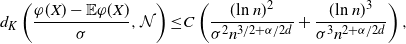 \begin{align} d_K \left( \frac{ \varphi(X) - \mathbb{E} \varphi(X) }{\sigma }, \mathcal{N}\right)\leq & C\left( \frac{ (\text{ln}\ n)^{2} }{ \sigma^2 n^{3/2 + \alpha/2d}} + \frac{ (\text{ln}\ n)^3}{ \sigma^3 n^{2 + \alpha/2d}}\right),\end{align}
where
 $C > 0$
is a constant not depending on n.
$C > 0$
is a constant not depending on n.
The second result introduces bounds on the variance under some additional assumptions.
Proposition 4.2. Let
 $K \subseteq [0,1]^d$
satisfy the rolling ball condition. Moreover, assume that there exist
$K \subseteq [0,1]^d$
satisfy the rolling ball condition. Moreover, assume that there exist
 $S_-(K), \, S_+(K), \, \alpha > 0$
such that
$S_-(K), \, S_+(K), \, \alpha > 0$
such that
 \begin{align}\notag S_+(K)r^{\alpha} \leq Vol(\partial K^r) \leq S_+(K)r^{\alpha} \quad { for\ every }\ r > 0.\end{align}
Then, for n sufficiently large,
 \begin{align} C_d^- S_- (K) \gamma(K) \leq \frac{Var ( \varphi(X)) }{n^{-1 - \alpha/d} } \leq C_d^+ S_+ (K)\end{align}
for some
 $C_d^-, C_d^+ > 0$
.
$C_d^-, C_d^+ > 0$
.
It is clear that Theorem 4.1 will be proved once Proposition 4.1 and Proposition 4.2 are established.
4.1. Proof of Proposition 4.1
Again, as before, we introduce a set of instructions R and a function h such that
 $h(R) = \varphi(X)$
. We apply Proposition 2.1, and the initial step is to bound
$h(R) = \varphi(X)$
. We apply Proposition 2.1, and the initial step is to bound
 $\mathbb{E}|\Delta_i h(R)|^r$
, where
$\mathbb{E}|\Delta_i h(R)|^r$
, where
 $ r > 0$
. In fact, the following holds.
$ r > 0$
. In fact, the following holds.
Proposition 4.3. Under the assumptions of Proposition 4.1,
 \begin{align} \mathbb{E} |\Delta_i h(R)|^r \leq c_{d,r, \alpha} S_+(K) (\text{ln}\ n)^r n^{- r - \alpha /d},\end{align}
where
 $c_{d,r , \alpha}$
depends on the parameters of the model and the dimension d, as well as on r and
$c_{d,r , \alpha}$
depends on the parameters of the model and the dimension d, as well as on r and
 $\alpha$
. Moreover, for
$\alpha$
. Moreover, for
 $n,q \geq 1$
,
$n,q \geq 1$
,
 \begin{align} \mathbb{E} |\varphi(X) - \mathbb{E} \varphi(X) |^r \leq C_{d, r, \alpha} S_+ (K) (\text{ln}\ n)^{r} n^{-r/2 - \alpha /d}\end{align}
for some
 $C_{d, r, \alpha} > 0$
.
$C_{d, r, \alpha} > 0$
.
Before presenting the proof, we introduce some notation. Recall that
 $x, y \in [0,1]^d$
are said to be Voronoi neighbors within the set X if
$x, y \in [0,1]^d$
are said to be Voronoi neighbors within the set X if
 $V(x;\, X) \cap V(y;\, X) \neq \emptyset$
. In general, the Voronoi distance
$V(x;\, X) \cap V(y;\, X) \neq \emptyset$
. In general, the Voronoi distance
 $d_V(x, y;\, X)$
between x and y within X is given by the smallest
$d_V(x, y;\, X)$
between x and y within X is given by the smallest
 $k \geq 1$
such that there exist
$k \geq 1$
such that there exist
 $x = x_0, x_1 \in X, \ldots, x_{k-1} \in X, x_k = y$
such that
$x = x_0, x_1 \in X, \ldots, x_{k-1} \in X, x_k = y$
such that
 $x_i, x_{i+1}$
are Voronoi neighbors for
$x_i, x_{i+1}$
are Voronoi neighbors for
 $i = 0, \ldots, k-1$
.
$i = 0, \ldots, k-1$
.
Denote by
 $v(x, y;\, X) = Vol\big(V(y;\, X) \cap V(x;\, (y, X)) \big)$
the volume that
$v(x, y;\, X) = Vol\big(V(y;\, X) \cap V(x;\, (y, X)) \big)$
the volume that
 $V(y;\,X)$
loses when x is added to X. Then, for
$V(y;\,X)$
loses when x is added to X. Then, for
 $x \notin X$
,
$x \notin X$
,
 \begin{align}\notag \varphi(X, x) - \varphi(X) = \mathbf{1}_{x \in K} \sum_{y \in X \cap K^c} v(x, y;\, X) - \mathbf{1}_{x \in K^c} \sum_{y \in X \cap K} v(x, y;\, X).\end{align}
Let
 $R_k(x;\, X)$
be the distance from x to the farthest point in the cell of a kth-order Voronoi neighbor in X; i.e., for
$R_k(x;\, X)$
be the distance from x to the farthest point in the cell of a kth-order Voronoi neighbor in X; i.e., for
 $X = (X_1, \ldots, X_n)$
,
$X = (X_1, \ldots, X_n)$
,
 \begin{align}\notag R_k(x;\, X) = \sup \big\{ || y - x|| \,:\, y \in V\big(X_i;\, X\big), d_V\big(x, X_i;\, X\big) \leq k\big\},\end{align}
with
 $R(x;\, X) \,{:}\,{\raise-1.5pt{=}}\, R_1(x;\, X)$
. If x does not have kth-order neighbors, take
$R(x;\, X) \,{:}\,{\raise-1.5pt{=}}\, R_1(x;\, X)$
. If x does not have kth-order neighbors, take
 $R_k(x;\, X) = \sqrt{d}$
. Then
$R_k(x;\, X) = \sqrt{d}$
. Then
 \begin{align}\notag Vol(V(x;\, X)) \leq \kappa_d R(x;\, X)^d,\end{align}
where
 $\kappa_d = \pi^{d/2} / \Gamma(d/2 + 1)$
is the volume of the unit ball in
$\kappa_d = \pi^{d/2} / \Gamma(d/2 + 1)$
is the volume of the unit ball in
 $\mathbb{R}^d$
.
$\mathbb{R}^d$
.
Proof of Proposition 4.3. The proof relies on two results. First, we have the following technical lemma which is established in Section 5.6.
Lemma 4.1. Assume there exist
 $S_+(K), \alpha > 0$
such that
$S_+(K), \alpha > 0$
such that
 $Vol(\partial K^r) \leq S_+(K) r^{\alpha}$
for all
$Vol(\partial K^r) \leq S_+(K) r^{\alpha}$
for all
 $r > 0$
. Let
$r > 0$
. Let
 \begin{align}\notag U_k(i) = \mathbf{1}_{d\big(X_i, \partial K\big) \leq R_k\big(X_i;\, X\big)} R_k\big(X_i;\, X\big)^d.\end{align}
Then, for some
 $c_{d, qd + \alpha, k} >0$
,
$c_{d, qd + \alpha, k} >0$
,
 \begin{align}\notag \mathbb{E} U_k^q(i) \leq S_+ (K) c_{d,q d + \alpha, k} n^{- q - \alpha/d}\end{align}
for all
 $n \geq 1$
,
$n \geq 1$
,
 $q \geq 1$
.
$q \geq 1$
.
Second, within our framework, we have the following version of [Reference Lachièze-Rey and Peccati14, Proposition 6.4] where S(R) is the original set of points generated by R and
 $S(R^i)$
is the set of points generated after the change in the instruction
$S(R^i)$
is the set of points generated after the change in the instruction
 $R_i$
.
$R_i$
.
Proposition 4.4. (i) If, for every
 $s \in S(R) \setminus S\big(R^i\big)$
, the set
$s \in S(R) \setminus S\big(R^i\big)$
, the set
 $R_1(s, S(R))$
, which contains s and all its neighbors, is either entirely in K or entirely in
$R_1(s, S(R))$
, which contains s and all its neighbors, is either entirely in K or entirely in
 $K^c$
, then
$K^c$
, then
 $\Delta_i h(R)= 0$
. A similar result holds for
$\Delta_i h(R)= 0$
. A similar result holds for
 $s \in S\big(R^i\big) \setminus S(R)$
and the set
$s \in S\big(R^i\big) \setminus S(R)$
and the set
 $R_1\big(s, S\big(R^i\big)\big)$
.
$R_1\big(s, S\big(R^i\big)\big)$
.
(ii) Assume
 $|i - j|$
is large enough so that
$|i - j|$
is large enough so that
 $(S\big(R^i\big) \setminus S(R) ) \cup (S(R^j) \setminus S(R)) = S\big(R^{ij}\big) \setminus S(R)$
, where
$(S\big(R^i\big) \setminus S(R) ) \cup (S(R^j) \setminus S(R)) = S\big(R^{ij}\big) \setminus S(R)$
, where
 $S\big(R^{ij}\big)$
is the set of points generated after the changes in both
$S\big(R^{ij}\big)$
is the set of points generated after the changes in both
 $R_i$
and
$R_i$
and
 $R_j$
. Suppose that for every
$R_j$
. Suppose that for every
 $s_1 \in S\big(R^i\big) \Delta S(R)$
and
$s_1 \in S\big(R^i\big) \Delta S(R)$
and
 $s_2 \in S\big(R^j\big) \Delta S(R)$
, at least one of the following holds:
$s_2 \in S\big(R^j\big) \Delta S(R)$
, at least one of the following holds:
-
1.
$d_V( s_1, s_2;\, S\big(R^{ij}\big) \cap S(R)) \geq 2$
, or -
2.
$d_V\big(s_1, \partial K;\, S\big(R^{ij}\big) \cap S(R)\big) \geq 2$
and
$d_V\big(s_2, \partial K;\, S\big(R^{ij}\big) \cap S(R) \big) \cap S(R)) \geq 2$
.

Then
 $\Delta_{i,j} h(R) = 0$
.
$\Delta_{i,j} h(R) = 0$
.
Now, write
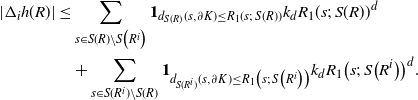 \begin{align}\notag |\Delta_i h(R)| \leq & \sum_{s \in S(R) \setminus S\big(R^i\big)} \mathbf{1}_{d_{S(R)}(s, \partial K) \leq R_1(s;\, S(R))} k_d R_1(s;\, S(R))^d \\\notag & + \sum_{s \in S(R^i) \setminus S(R)} \mathbf{1}_{d_{S(R^i)}(s, \partial K) \leq R_1\big(s;\, S\big(R^i\big)\big)} k_d R_1\big(s;\, S\big(R^i\big)\big)^d.\end{align}
As before, for some
 $T > 0$
, there exist an event E and
$T > 0$
, there exist an event E and
 $\epsilon > 0$
such that, conditioned on E,
$\epsilon > 0$
such that, conditioned on E,
 $|S(R^i) \setminus S(R)| = |S(R) \setminus S(R^i)| \leq T$
and
$|S(R^i) \setminus S(R)| = |S(R) \setminus S(R^i)| \leq T$
and
 $\mathbb{P}(E^c) \leq (1 - \epsilon)^T$
. Then, from Lemma 4.1, there exist
$\mathbb{P}(E^c) \leq (1 - \epsilon)^T$
. Then, from Lemma 4.1, there exist
 $S_+(K), \alpha > 0$
such that
$S_+(K), \alpha > 0$
such that
 \begin{align}\notag \mathbb{E} |\Delta_i h(R)|^r \leq c_{d,r, \alpha} (1 - \epsilon)^T + c_{d,r, \alpha} S_+(K) T^r n^{- r - \alpha /d},\end{align}
where
 $c_{d,r , \alpha}$
depends on the parameters of the model and the dimension d, as well as on r and
$c_{d,r , \alpha}$
depends on the parameters of the model and the dimension d, as well as on r and
 $\alpha$
. If
$\alpha$
. If
 $T = c\text{ln}\ n$
for a suitable
$T = c\text{ln}\ n$
for a suitable
 $c > 0$
, then
$c > 0$
, then
 \begin{align}\notag \mathbb{E} |\Delta_i h(R)|^r \leq c_{d,r, \alpha} S_+(K) (\text{ln}\ n)^r n^{- r - \alpha /d},\end{align}
as desired. An application of the rth-moment Efron–Stein inequality (see [Reference Houdré and Ma12, Reference Rhee and Talagrand16]) then yields (23).
For the non-variance term in Theorem 2.1, we have
 \begin{align} \frac{1}{4 \sigma^3} \sum_{j = 0}^{|R| - 1} \sqrt{\mathbb{E} | \Delta_j h(R)|^6} + \frac{\sqrt{2 \pi} } {16 \sigma^3} \sum_{j = 0}^{|R| - 1} \mathbb{E} |\Delta_j h(R)|^3 \leq C \sigma^{-3} (\text{ln}\ n)^3 n^{- 2 - \alpha /2d}.\end{align}
To analyze the bound on the variance terms given by Proposition 2.3, first note that
 \begin{align}\notag \sum_{i = 0}^{|R| -1} \sum_{j, k \notin A} \mathbf{1}_{i = j = k} \mathbb{E} | \Delta_i h(R)|^4 \leq C(\text{ln}\ n)^4 n^{- 3 - \alpha /d},\end{align}
again using Proposition 4.3. The other terms are bounded as follows.
Proposition 4.5. Let
 $A \subsetneq [ | R | ] $
, and let
$A \subsetneq [ | R | ] $
, and let
 $B_{|R|}(h), B_{|R|}^k(h)$
and
$B_{|R|}(h), B_{|R|}^k(h)$
and
 $B_{|R|}^j(h)$
be as in (6). Then, for
$B_{|R|}^j(h)$
be as in (6). Then, for
 $\epsilon > 0$
,
$\epsilon > 0$
,
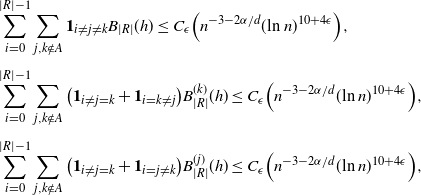 \begin{align}\notag \sum_{i = 0}^{|R| -1} & \sum_{j, k \notin A} \mathbf{1}_{i \neq j \neq k} B_{|R|}(h) \leq C_\epsilon \Big( n^{-3 - 2 \alpha/d} (\text{ln}\ n)^{10 + 4 \epsilon}\Big), \\[4pt]\notag \sum_{i = 0}^{|R| -1} & \sum_{j, k \notin A} \big(\mathbf{1}_{i \neq j = k} + \mathbf{1}_{i = k \neq j} \big) B_{|R|}^{(k)}(h) \leq C_\epsilon \Big( n^{-3 - 2 \alpha/d} (\text{ln}\ n)^{10 + 4 \epsilon}\Big) , \\[4pt]\notag \sum_{i = 0}^{|R| -1} & \sum_{j, k \notin A} \big(\mathbf{1}_{i \neq j = k} + \mathbf{1}_{i = j \neq k} \big) B_{|R|}^{(j)}(h) \leq C_\epsilon \Big( n^{-3 - 2 \alpha/d} (\text{ln}\ n)^{10 + 4 \epsilon}\Big) ,\end{align}
for some constant
 $C_\epsilon> 0$
that does not depend on n.
$C_\epsilon> 0$
that does not depend on n.
Proof. See Section 5.7 for the proof of the first bound. The others follow similarly.
The bounds on the variance terms in Proposition 2.3 become
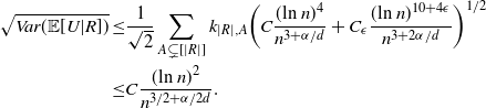 \begin{align}\notag \sqrt{Var(\mathbb{E}[U|R])} \leq & \frac{1}{\sqrt{2}} \sum_{A \subsetneq[|R|]} k_{|R|, A} \bigg( C \frac{(\text{ln}\ n)^4}{n^{3 + \alpha/d} } + C_\epsilon \frac{(\text{ln}\ n)^{10 + 4 \epsilon}}{n^{3 + 2\alpha /d}} \bigg)^{1/2}\\ \leq & C \frac{(\text{ln}\ n)^2 }{n^{3/2 + \alpha/2d}}.\end{align}
4.2. Proof of Proposition 4.2
The upper bound follows immediately from Proposition 4.3.
Recall the following result ([Reference Lachièze-Rey and Peccati14, Corollary 2.4]) concerning the variance. Let
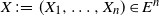 $X \,{:}\,{\raise-1.5pt{=}}\, (X_1, \ldots, X_n) \in E^n$
, where E is a Polish space. If X
′ is an independent copy of X, and
$X \,{:}\,{\raise-1.5pt{=}}\, (X_1, \ldots, X_n) \in E^n$
, where E is a Polish space. If X
′ is an independent copy of X, and
 $f\,:\, E^n \to \mathbb{R}$
is measurable, with
$f\,:\, E^n \to \mathbb{R}$
is measurable, with
 $\mathbb{E}\big[ f(X)^2\big] < \infty$
,
$\mathbb{E}\big[ f(X)^2\big] < \infty$
,
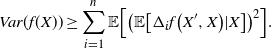 \begin{align} Var(f(X)) \geq \sum_{i = 1}^n \mathbb{E}\Big[ \big( \mathbb{E} \big[ \Delta_i f\big(X^{\prime},X\big) |X \big] \big)^2\Big].\end{align}
In our setting we take
 $f = \varphi$
. Unlike in [Reference Lachièze-Rey and Peccati14], the function
$f = \varphi$
. Unlike in [Reference Lachièze-Rey and Peccati14], the function
 $\varphi$
is not symmetric, and the right-hand side of (26) cannot be simplified. The lower bound provided by [Reference Lachièze-Rey and Peccati14, Corollary 2.4] recovers the correct order of growth of the variance, which is enough for our purposes. However, more precise generic results are also available; see e.g. [Reference Bousquet and Houdré1].
$\varphi$
is not symmetric, and the right-hand side of (26) cannot be simplified. The lower bound provided by [Reference Lachièze-Rey and Peccati14, Corollary 2.4] recovers the correct order of growth of the variance, which is enough for our purposes. However, more precise generic results are also available; see e.g. [Reference Bousquet and Houdré1].
Let H be the realization of the hidden chain for X. By the law of total variance,
 $Var(\varphi(X)) \geq Var(\varphi(X) | H)$
. Let X
′ be an independent copy of X, given H. Note that, given H,
$Var(\varphi(X)) \geq Var(\varphi(X) | H)$
. Let X
′ be an independent copy of X, given H. Note that, given H,
 $(X_i)_{i = 1, \ldots, n}$
and
$(X_i)_{i = 1, \ldots, n}$
and
 $\big(X^{\prime}_i\big)_{ i = 1, \ldots, n}$
are independent random variables which are not identically distributed.
$\big(X^{\prime}_i\big)_{ i = 1, \ldots, n}$
are independent random variables which are not identically distributed.
Applying (26) to
 $\varphi(X | H)$
, we obtain
$\varphi(X | H)$
, we obtain
 \begin{align}\notag Var(\varphi(X) | H) \geq \sum_{i = 1}^n \mathbb{E}_{X^{\prime}_i}^H \Big( \mathbb{E}_X^H \big[ \varphi\big(X^i\big) - \varphi(X) \big] \Big)^2,\end{align}
where
 $X^i = \big(X_1, \ldots, X_{i-1}, X^{\prime}_i, X_{i+1}, \ldots, X_n\big)$
, and
$X^i = \big(X_1, \ldots, X_{i-1}, X^{\prime}_i, X_{i+1}, \ldots, X_n\big)$
, and
 $\mathbb{E}^H$
indicates that H is given. (To simplify notation in what follows we drop the H.) The difference from the proof in [Reference Lachièze-Rey and Peccati14] is that now the variables are no longer identically distributed. Write
$\mathbb{E}^H$
indicates that H is given. (To simplify notation in what follows we drop the H.) The difference from the proof in [Reference Lachièze-Rey and Peccati14] is that now the variables are no longer identically distributed. Write
 \begin{align}\notag \mathbb{E}_X \big[ \varphi\big(X^i\big) - \varphi(X) \big] = \mathbb{E}_X \big[ \varphi\big(X^i\big) - \varphi\big(X^{(i)}\big)\big] - \mathbb{E}_X\big[ \varphi(X) - \varphi\big(X^{(i)}\big)\big],\end{align}
where
 $X^{(i)} = \big(X_1, \ldots, X_{i-1}, X_{i+1}, \ldots, X_n\big)$
. By Lemma 4.1,
$X^{(i)} = \big(X_1, \ldots, X_{i-1}, X_{i+1}, \ldots, X_n\big)$
. By Lemma 4.1,
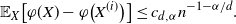 \begin{align} \mathbb{E}_X\big[ \varphi(X) - \varphi\big(X^{(i)}\big)\big] \leq c_{d, \alpha} n^{-1 - \alpha/d}.\end{align}
We are left to study
 $\mathbb{E} \big[ \varphi\big(X^i\big) - \varphi\big(X^{(i)}\big)\big]$
. Recall that
$\mathbb{E} \big[ \varphi\big(X^i\big) - \varphi\big(X^{(i)}\big)\big]$
. Recall that
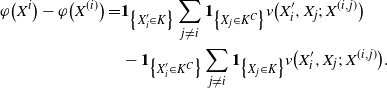 \begin{align}\notag \varphi\big(X^i\big) - \varphi\big(X^{(i)}\big) = & \mathbf{1}_{\big\{X^{\prime}_i \in K\big\}} \sum_{j \neq i} \mathbf{1}_{\big\{X_j \in K^C\big\}} v\big(X^{\prime}_i, X_j;\, X^{(i,j)}\big) \\\notag & - \mathbf{1}_{\big\{X^{\prime}_i \in K^C\big\}} \sum_{j \neq i} \mathbf{1}_{\big\{X_j \in K\big\}} v\big(X^{\prime}_i, X_j;\, X^{(i,j)}\big).\end{align}
Now, for the case
 $X^{\prime}_i \in K^C$
(the other case being equivalent), we have
$X^{\prime}_i \in K^C$
(the other case being equivalent), we have
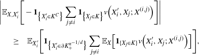 \begin{align}\notag \Bigg|\mathbb{E}_{X, X^{\prime}_i} & \Bigg[ - \mathbf{1}_{\big\{X^{\prime}_i \in K^C\big\}} \sum_{j \neq i} \mathbf{1}_{\big\{X_j \in K\big\}} v\Big(X^{\prime}_i, X_j;\, X^{(i,j)}\Big) \Bigg] \Bigg| \\\notag \geq & \quad \mathbb{E}_{X^{\prime}_i} \Bigg[\mathbf{1}_{\big\{X^{\prime}_i \in \partial K_+^{n^{-1/d}} \big\}} \sum_{j \neq i} \mathbb{E}_X\Big[ \mathbf{1}_{\{X_j \in K\}} v\Big(X^{\prime}_i, X_j;\, X^{(i,j)}\Big) \Big] \Bigg],\end{align}
since
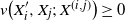 $v\big(X^{\prime}_i, X_j;\, X^{(i,j)}\big) \geq 0$
. Then
$v\big(X^{\prime}_i, X_j;\, X^{(i,j)}\big) \geq 0$
. Then
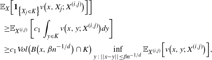 \begin{align}\notag \mathbb{E}_X & \Big[ \mathbf{1}_{\big\{X_j \in K\big\}} v\big(x, X_j;\, X^{(i,j)}\big) \Big]\Big ] \\\notag \geq & \mathbb{E}_{X^{(i,j)}} \left[ c_1 \int_{y \in K} v\big(x, y;\, X^{(i,j)}\big) dy \right] \\\notag \geq & c_1 Vol\big(B\big(x, \beta n^{-1/d}\big) \cap K\big) \inf_{y \,:\, ||x- y || \leq \beta n^{-1/d}} \mathbb{E}_{X^{(i,j)}}\Big[ v\big(x,y;\, X^{(i,j)}\big)\Big],\end{align}
using the independence after conditioning on H and the properties of the model. We want to find an event that implies that
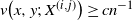 $v\big(x,y;\, X^{(i,j)}\big) \geq c n^{-1}$
. One instance is when no point of
$v\big(x,y;\, X^{(i,j)}\big) \geq c n^{-1}$
. One instance is when no point of
 $X^{(i,j)}$
falls in
$X^{(i,j)}$
falls in
 $B\big(y, 6 \beta n^{-1/d}\big)$
. Indeed, then
$B\big(y, 6 \beta n^{-1/d}\big)$
. Indeed, then
 $B\big(y, 3 \beta n^{-1/d}\big) \subset V\big(y, X^{(i,j)}\big)$
. The distance between y and x is less than
$B\big(y, 3 \beta n^{-1/d}\big) \subset V\big(y, X^{(i,j)}\big)$
. The distance between y and x is less than
 $\beta n^{-1/d}$
, and so there is
$\beta n^{-1/d}$
, and so there is
 $z \in B\big(y, 3 \beta n^{-1/d}\big)$
, namely
$z \in B\big(y, 3 \beta n^{-1/d}\big)$
, namely
 $z = x + \beta n^{-1/d} (x - y)/||x-y||$
, such that
$z = x + \beta n^{-1/d} (x - y)/||x-y||$
, such that
 \begin{align}\notag B\big(z, \beta n^{-1/d}\big) \subset V\big(x, \big(X^{(i,j)}, y\big)\big) \subset B\big(y, 3 \beta n^{-1/d}\big) \subset V\big(y;\, X^{(i,j)}\big).\end{align}
Then
 $v\big(x,y;\, X^{(i,j)}\big) \geq Vol\big(B\big(z, \beta n^{-1/d}\big) = \kappa_d \beta^d n^{-1}$
. Finally,
$v\big(x,y;\, X^{(i,j)}\big) \geq Vol\big(B\big(z, \beta n^{-1/d}\big) = \kappa_d \beta^d n^{-1}$
. Finally,
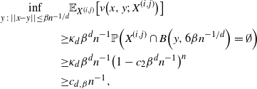 \begin{align}\notag \inf_{y \,:\, ||x- y || \leq \beta n^{-1/d}} & \mathbb{E}_{X^{(i,j)}}\big[ v\big(x,y;\, X^{(i,j)}\big)\big] \\\notag \geq & \kappa_d \beta^d n^{-1} \mathbb{P} \Big( X^{(i,j)} \cap B\Big(y, 6 \beta n^{-1/d}\Big) = \emptyset\Big) \\\notag \geq & \kappa_d \beta^d n^{-1} \big( 1 - c_2 \beta^d n^{-1}\big)^n \\\notag \geq & c_{d, \beta} n^{-1},\end{align}
for some
 $c_{d, \beta} > 0$
depending on the parameters of the model, the dimension d, and
$c_{d, \beta} > 0$
depending on the parameters of the model, the dimension d, and
 $ \beta$
. Then
$ \beta$
. Then
 \begin{align}\notag \mathbb{E}_X \Big[ \mathbf{1}_{\big\{X_j \in K\big\}} v\big(x, X_j;\, X^{(i,j)}\big) \Big]\Big ] \geq c_{d, \beta} Vol\big(B\big(x, \beta n^{-1/d}\big) \big) n^{-1}.\end{align}
Therefore, by the very definition of
 $\gamma(K, r, \beta)$
and since the case
$\gamma(K, r, \beta)$
and since the case
 $X^{\prime}_i \in K$
is symmetric,
$X^{\prime}_i \in K$
is symmetric,
 \begin{align}\notag \mathbb{E}_{X^{\prime}_i} \mathbb{E}_X \Big[ \big(\varphi\big(X^i\big) - \varphi\big(X^{(i)}\big)^2\Big ] \geq & c_{d, \beta} \bigg( c_1 \int_{\partial K_+^{n^{-1/d}} } Vol\big(B \big( x, \beta n^{-1/d}\big) \cap K\big)^2 dx \\\notag & \quad + c_1 \int_{\partial K_-^{n^{-1/d}} } Vol\big(B \big( x, \beta n^{-1/d}\big) \cap K^c\big)^2 dx\bigg) \\\notag = & c_{d, \beta} \big( n^{-2} \gamma\big(K, n^{-1/d}, \beta\big) + n^{-2} \gamma\big(K^c, n^{-1/d}, \beta\big) \big).\end{align}
If the rolling ball condition (18) and the lower bound on
 $\partial{K}^{n^{-1/d}}$
both hold, then
$\partial{K}^{n^{-1/d}}$
both hold, then
 \begin{align}\notag \mathbb{E}_{X^{\prime}_i} \mathbb{E}_X \Big[ \big(\varphi\big(X^i\big) - \varphi\big(X^{(i)}\big)^2 \Big] \geq c_{d, \beta} S_-(K) \gamma(K, \beta) n^{-2 - \alpha/d},\end{align}
which dominates the contribution (27) from
 $\mathbb{E}\big[\varphi (X) - \varphi\big(X^{(i)}\big)\big]$
. Therefore, finally,
$\mathbb{E}\big[\varphi (X) - \varphi\big(X^{(i)}\big)\big]$
. Therefore, finally,
 \begin{align}\notag Var(\varphi(X)) \geq c_{d, \beta}^- S_-(K) \gamma(K, \beta) n^{-1 - \alpha/d},\end{align}
as desired.
Remark 4.1. Let us expand a bit on another potential application of our generic framework, namely the occupancy problem as studied in [Reference Grabchak, Kelbert and Paris10]. To set up the notation,
 $(Z_1, \ldots, Z_n)$
is an aperiodic, irreducible, and time-homogeneous (hidden) Markov chain that transitions between different alphabets. To each alphabet is associated a distribution over the collection of all possible letters, giving rise to the observed letters
$(Z_1, \ldots, Z_n)$
is an aperiodic, irreducible, and time-homogeneous (hidden) Markov chain that transitions between different alphabets. To each alphabet is associated a distribution over the collection of all possible letters, giving rise to the observed letters
 $(X_1, \ldots, X_n)$
. We assume that the number of alphabets is finite but that the number of total letters is
$(X_1, \ldots, X_n)$
. We assume that the number of alphabets is finite but that the number of total letters is
 $\lfloor\alpha n\rfloor$
, for some fixed
$\lfloor\alpha n\rfloor$
, for some fixed
 $\alpha >0$
. One studies
$\alpha >0$
. One studies
 $W \,{:}\,{\raise-1.5pt{=}}\, f(X_1, \ldots, X_n)$
—the number of letters that have not appeared among the
$W \,{:}\,{\raise-1.5pt{=}}\, f(X_1, \ldots, X_n)$
—the number of letters that have not appeared among the
 $X_1, \ldots, X_n$
. Then an analysis as in the proof of Theorem 3.1 leads to the following:
$X_1, \ldots, X_n$
. Then an analysis as in the proof of Theorem 3.1 leads to the following:
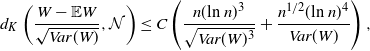 \begin{align}\notag d_K\left(\frac{W - \mathbb{E} W}{\sqrt{Var (W)}} , \mathcal{N} \right) \leq C \left( \frac{ n(\text{ln}\ n)^3} {\sqrt{Var(W)^3}} + \frac{ n^{1/2} (\text{ln}\ n)^4}{ Var(W)} \right),\end{align}
where Var(W) is a function of n,
 $\mathcal{N}$
is the standard normal distribution, and
$\mathcal{N}$
is the standard normal distribution, and
 $C > 0$
is a constant depending on the parameters of the model but not on n. As mentioned at the beginning of the section, the study of the precise order of growth of the variance of W, in our dependent framework, is not within the scope of the current paper. For the i.i.d. case one can show (see e.g. [Reference Englund8]) that
$C > 0$
is a constant depending on the parameters of the model but not on n. As mentioned at the beginning of the section, the study of the precise order of growth of the variance of W, in our dependent framework, is not within the scope of the current paper. For the i.i.d. case one can show (see e.g. [Reference Englund8]) that
 $Var(W) \sim \big(\alpha e^{-1/ \alpha} - (1 + \alpha) e^{-2 / \alpha} \big) n$
as
$Var(W) \sim \big(\alpha e^{-1/ \alpha} - (1 + \alpha) e^{-2 / \alpha} \big) n$
as
 $n \to \infty$
.
$n \to \infty$
.
5. Technical results
5.1. Bounds on terms involving
$\Delta_i h$

Recall the setting of Proposition 2.2 and Proposition 2.3. Let (Z, X) be a hidden Markov model and let the latent chain Z be irreducible and aperiodic, with finite state space
 $\mathcal{S}$
. Assume that Z is started at the stationary distribution.
$\mathcal{S}$
. Assume that Z is started at the stationary distribution.
We start by establishing a technical result regarding Z.
First, note that there exist
 $K \geq 1$
and
$K \geq 1$
and
 $\epsilon \in (0,1)$
such that
$\epsilon \in (0,1)$
such that
 \begin{align}\notag \mathbb{P} \big(Z_n = s, Z_{n + K} = s^{\prime}\big) \geq \epsilon,\end{align}
and thus,
 \begin{align} \mathbb{P}\big(Z_{n + K} = s^{\prime}\big) \geq \epsilon, \quad \mathbb{P}\big(Z_{n+K} = s^{\prime} | Z_n = s\big) \geq \epsilon\end{align}
for all
 $n \geq 1$
and
$n \geq 1$
and
 $s, s^{\prime} \in \mathcal{S}$
.
$s, s^{\prime} \in \mathcal{S}$
.
Lemma 5.1. Let
 $K \geq 1$
and
$K \geq 1$
and
 $\epsilon \in (0,1)$
be as in (28), and let
$\epsilon \in (0,1)$
be as in (28), and let
 $(Z_i)_{i \geq 1}$
be an irreducible and aperiodic Markov chain with finite state space
$(Z_i)_{i \geq 1}$
be an irreducible and aperiodic Markov chain with finite state space
 $\mathcal{S}$
. Then
$\mathcal{S}$
. Then
 \begin{align} \mathbb{P}\left(Z_{j+K} \neq s_1, Z_{j+2K} \neq s_2, \ldots, Z_{j+tK} \neq s_t\right) \leq (1 - \epsilon)^t\end{align}
for any
 $t \geq 1$
,
$t \geq 1$
,
 $j \geq 1$
, and
$j \geq 1$
, and
 $(s_1, \ldots, s_t) \in \mathcal{S}^t$
.
$(s_1, \ldots, s_t) \in \mathcal{S}^t$
.
Proof. We show (29) by induction. The case
 $t = 1$
follows from (28). Next, for
$t = 1$
follows from (28). Next, for
 $(s_1, \ldots, s_{t+1}) \in \mathcal{S}^{t+1}$
,
$(s_1, \ldots, s_{t+1}) \in \mathcal{S}^{t+1}$
,
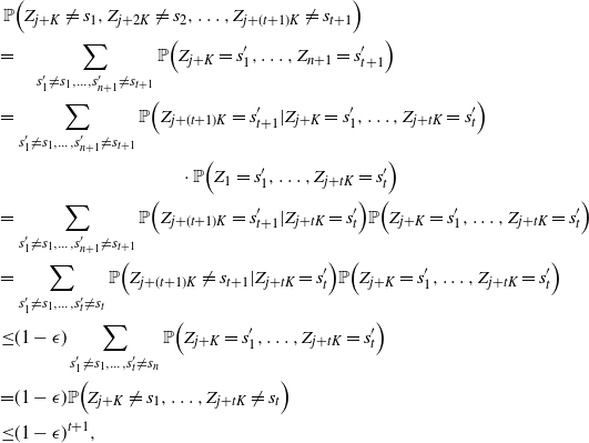 \begin{align}\notag \mathbb{P}& \Big(Z_{j+K} \neq s_1, Z_{j+2K} \neq s_2, \ldots, Z_{j+(t+1)K} \neq s_{t+1}\Big) \\\notag = & \quad \sum_{s^{\prime}_1 \neq s_1, \ldots, s^{\prime}_{n+1} \neq s_{t+1} } \mathbb{P} \Big(Z_{j+K} = s^{\prime}_1, \ldots, Z_{n+1} = s^{\prime}_{t+1}\Big) \\\notag = & \sum_{s^{\prime}_1 \neq s_1, \ldots, s^{\prime}_{n+1} \neq s_{t+1} } \mathbb{P} \Big(Z_{j+(t+1)K} = s^{\prime}_{t+1} | Z_{j+K} = s^{\prime}_1, \ldots, Z_{j + tK} = s^{\prime}_{t}\Big) \\\notag & \quad \quad \quad \quad\quad\quad \quad\quad \quad \cdot \mathbb{P} \Big( Z_1 = s^{\prime}_1, \ldots, Z_{j + tK} = s^{\prime}_{t}\Big) \\\notag = & \sum_{s^{\prime}_1 \neq s_1, \ldots, s^{\prime}_{n+1} \neq s_{t+1} } \mathbb{P} \Big(Z_{j+(t+1)K} = s^{\prime}_{t+1} | Z_{j + tK} = s^{\prime}_t\Big) \mathbb{P} \Big( Z_{j+K} = s^{\prime}_1, \ldots, Z_{j + tK} = s^{\prime}_{t}\Big) \\\notag = & \sum_{s^{\prime}_1 \neq s_1, \ldots, s^{\prime}_{t} \neq s_{t} } \mathbb{P} \Big(Z_{j+(t+1)K} \neq s_{t+1} | Z_{j + tK} = s^{\prime}_{t}\Big) \mathbb{P} \Big( Z_{j+K} = s^{\prime}_1, \ldots, Z_{j + tK} = s^{\prime}_{t}\Big) \\\notag \leq & (1 - \epsilon) \sum_{s^{\prime}_1 \neq s_1, \ldots, s^{\prime}_{t} \neq s_{n} } \mathbb{P} \Big( Z_{j+K} = s^{\prime}_1, \ldots, Z_{j + tK} = s^{\prime}_{t}\Big) \\\notag = & (1 - \epsilon) \mathbb{P} \Big(Z_{j+K} \neq s_1, \ldots, Z_{j + tK} \neq s_t\Big) \\\notag \leq & (1 - \epsilon)^{t+1},\end{align}
where we have used the Markov property, (28), and finally the induction hypothesis. This suffices for the proof of (29), and thus the proof of the lemma is complete.
Let
 $f\,:\, \mathcal{A}^n \to \mathbb{R}$
be Lipschitz, i.e., be such that
$f\,:\, \mathcal{A}^n \to \mathbb{R}$
be Lipschitz, i.e., be such that
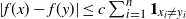 $|f(x) - f(y)| \leq c\sum_{i =1}^n \mathbf{1}_{x_i \neq y_i}$
for every
$|f(x) - f(y)| \leq c\sum_{i =1}^n \mathbf{1}_{x_i \neq y_i}$
for every
 $x, y \in \mathcal{A}^n$
, where
$x, y \in \mathcal{A}^n$
, where
 $c > 0$
. Let
$c > 0$
. Let
 $R = \big(R_0, \ldots, R_{|\mathcal{S}|(n-1)}\big)$
be a vector of independent random variables, and let h be the function such that
$R = \big(R_0, \ldots, R_{|\mathcal{S}|(n-1)}\big)$
be a vector of independent random variables, and let h be the function such that
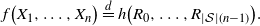 \begin{align}\notag f\big(X_1, \ldots, X_n\big) \overset{d}{=} h\big(R_0, \ldots, R_{|\mathcal{S}|(n-1)}\big).\end{align}
Let R ′ be an independent copy of R. The next result provides a tail inequality that is key for Proposition 2.2.
Proposition 5.1. Let
 $K > 0$
and
$K > 0$
and
 $\epsilon > 0$
be as in (28). Then
$\epsilon > 0$
be as in (28). Then
 \begin{align} \mathbb{P} (|\Delta_i h(R)| \geq c x ) \leq C (1 - \epsilon)^{x/K}\end{align}
for any
 $x \in \mathbb{N}$
, where
$x \in \mathbb{N}$
, where
 $C > 0$
depends on the parameters of the model but neither on n nor on x.
$C > 0$
depends on the parameters of the model but neither on n nor on x.
Proof. The sequence of instructions
 $R^i \,{:}\,{\raise-1.5pt{=}}\, \big(R_0, \ldots, R^{\prime}_i, \ldots, R_{|\mathcal{S}(n-1)|}\big)$
may give rise to a different realization (Z
′, X
′) of the hidden Markov model, as compared to (Z, X), the one generated by R. The two models are not independent. In particular, if instruction
$R^i \,{:}\,{\raise-1.5pt{=}}\, \big(R_0, \ldots, R^{\prime}_i, \ldots, R_{|\mathcal{S}(n-1)|}\big)$
may give rise to a different realization (Z
′, X
′) of the hidden Markov model, as compared to (Z, X), the one generated by R. The two models are not independent. In particular, if instruction
 $R_i$
determines
$R_i$
determines
 $\big(Z_j, X_j\big)$
and
$\big(Z_j, X_j\big)$
and
 $R^{\prime}_i$
determines
$R^{\prime}_i$
determines
 $\big(Z^{\prime}_j, X^{\prime}_j\big)$
, then
$\big(Z^{\prime}_j, X^{\prime}_j\big)$
, then
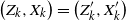 $\big(Z_k, X_k\big) = \big(Z^{\prime}_k, X^{\prime}_k\big)$
for
$\big(Z_k, X_k\big) = \big(Z^{\prime}_k, X^{\prime}_k\big)$
for
 $k < j$
. Let s be the smallest nonnegative integer (possibly
$k < j$
. Let s be the smallest nonnegative integer (possibly
 $s = \infty$
) such that
$s = \infty$
) such that
 $Z_{j+s} = Z^{\prime}_{j+s}$
. Then for any
$Z_{j+s} = Z^{\prime}_{j+s}$
. Then for any
 $k > j+s$
,
$k > j+s$
,
 $\big(Z_k, X_k\big) = \big(Z^{\prime}_k, X^{\prime}_k\big)$
as well. Finally, if
$\big(Z_k, X_k\big) = \big(Z^{\prime}_k, X^{\prime}_k\big)$
as well. Finally, if
 $k \in \{j, \ldots, j + s - 1\}$
, the pairs
$k \in \{j, \ldots, j + s - 1\}$
, the pairs
 $\big(Z_k, X_k\big)$
and
$\big(Z_k, X_k\big)$
and
 $\big(Z^{\prime}_k, X^{\prime}_k\big)$
are independent. We show next that for
$\big(Z^{\prime}_k, X^{\prime}_k\big)$
are independent. We show next that for
 $K \geq 1$
as in (28), and any
$K \geq 1$
as in (28), and any
 $t \in \mathbb{N}$
,
$t \in \mathbb{N}$
,
 \begin{align} \mathbb{P}(s \geq tK) \leq (1 - \epsilon)^t.\end{align}
Indeed,
 \begin{align}\notag \mathbb{P}(s > tK) \leq & \quad \mathbb{P} \left(Z_{j + K} \neq Z^{\prime}_{j+K},Z_{j + 2K} \neq Z^{\prime}_{j+2K},\ldots, Z_{j + tK} \neq Z^{\prime}_{j+tK} \right) \\\notag = & \quad \sum_{(s_1, \ldots, s_t) \in \mathcal{S}^t} \mathbb{P} \left(Z_{j + K} \neq s_1, Z^{\prime}_{j+K} = s_1, \ldots, Z_{j + tK} \neq s_t, Z^{\prime}_{j+tK} = s_t\right).\end{align}
By independence,
 \begin{align}\notag \mathbb{P} & \left(Z_{j + K} \neq s_1, Z^{\prime}_{j+K} = s_1, \ldots, Z_{j + tK} \neq s_t, Z^{\prime}_{j+tK} = s_t\right) \\\notag = & \quad \mathbb{P}\Big(Z_{j+K} \neq s_1, \ldots, Z_{j + tK} \neq s_t\Big) \mathbb{P}\Big(Z^{\prime}_{j+K} = s_1, \ldots, Z^{\prime}_{j+ tK} = s_t\Big),\end{align}
and thus by Lemma 5.1
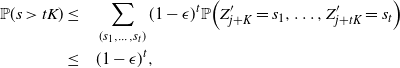 \begin{align}\notag \mathbb{P}(s > tK) \leq& \quad \sum_{(s_1, \ldots, s_t)} ( 1- \epsilon)^t \mathbb{P}\Big(Z^{\prime}_{j+K} = s_1, \ldots, Z^{\prime}_{j + tK} = s_t\Big) \\\notag \leq & \quad (1 - \epsilon)^t,\end{align}
as desired.
Let E(t) be the event
 \begin{align}\notag E(t) \,{:}\,{\raise-1.5pt{=}}\, \Big\{X_{j + K} \neq X^{\prime}_{j + K}, X_{j + 2K} \neq X^{\prime}_{j + 2K}, \ldots, X_{j + tK} \neq X^{\prime}_{j + tK}\Big\}.\end{align}
Note that
 $\mathbb{P} ( E(t) ) \leq \mathbb{P}(s \geq tK) \leq (1 - \epsilon)^{t}$
. In particular, if
$\mathbb{P} ( E(t) ) \leq \mathbb{P}(s \geq tK) \leq (1 - \epsilon)^{t}$
. In particular, if
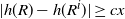 $|h(R) - h(R^i)| \geq cx$
, where
$|h(R) - h(R^i)| \geq cx$
, where
 $c > 0$
is the Lipschitz constant of the associated function f, then
$c > 0$
is the Lipschitz constant of the associated function f, then
 $s \geq x$
, as there are at least x positions k such that
$s \geq x$
, as there are at least x positions k such that
 $X_k \neq X^{\prime}_k $
. Thus,
$X_k \neq X^{\prime}_k $
. Thus,
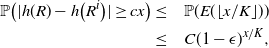 \begin{align}\notag \mathbb{P} \big( |h(R) - h\big(R^i\big) | \geq cx\big) \leq & \quad \mathbb{P} (E(\lfloor x/K \rfloor)) \\ \leq & \quad C (1 - \epsilon)^{x/K},\end{align}
where
 $C > 0$
depends on the parameters of the model but not on x. This suffices for the proof of (30).
$C > 0$
depends on the parameters of the model but not on x. This suffices for the proof of (30).
We now turn to the proof of Proposition 2.2.
Proof of Proposition 2.2. Let
 $E_t$
be the event that
$E_t$
be the event that
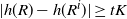 $|h(R) - h(R^i)| \geq tK$
. Then
$|h(R) - h(R^i)| \geq tK$
. Then
 \begin{align}\notag \mathbb{E} |h(R) - h\big(R^i\big)|^r = \mathbb{E} |h(R) - h\big(R^i\big)|^r \mathbf{1}_{E_t} + \mathbb{E} |h(R) - h\big(R^i\big)|^r \mathbf{1}_{E_t^c}.\end{align}
Recall that
 $|g(x)| \leq cn$
for all
$|g(x)| \leq cn$
for all
 $x \in \mathcal{A}^n$
, and then
$x \in \mathcal{A}^n$
, and then
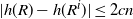 $|h(R) - h(R^i)| \leq 2cn$
. Using (32),
$|h(R) - h(R^i)| \leq 2cn$
. Using (32),
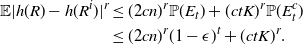 \begin{align}\notag \mathbb{E} |h(R) - h(R^i)|^r & \leq (2cn)^r \mathbb{P}(E_t) + (ctK)^r \mathbb{P}(E_t^c) \\ & \leq (2cn)^r (1 - \epsilon)^{t} + (ctK)^r.\end{align}
Let
 $t = - r \text{ln}\ n / (\text{ln}\ (1 - \epsilon) ) > 0$
. Then
$t = - r \text{ln}\ n / (\text{ln}\ (1 - \epsilon) ) > 0$
. Then
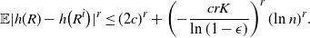 \begin{align} \mathbb{E}|h(R) - h\big(R^i\big) |^r \leq (2c)^r + \left( - \frac{ c r K }{\text{ln}\ (1 - \epsilon) } \right)^r (\text{ln}\ n)^r.\end{align}
The order of the bound is optimal for t such that
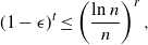 \begin{align} (1 - \epsilon)^{t } \leq \left( \frac{\text{ln}\ n}{n}\right)^r,\end{align}
or
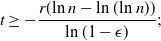 \begin{align}\notag t \geq - \frac{r (\text{ln}\ n - \text{ln}\ (\text{ln}\ n)) }{\text{ln}\ (1 - \epsilon)};\end{align}
it follows that
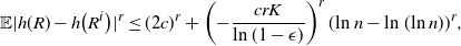 \begin{align}\notag \mathbb{E}|h(R) - h\big(R^i\big) |^r \leq (2c)^r + \left( - \frac{c r K }{\text{ln}\ (1 - \epsilon) } \right)^r (\text{ln}\ n - \text{ln}\ (\text{ln}\ n))^r,\end{align}
and the right-hand side has the same order of growth as (34).
If the growth order of
 $(1 - \epsilon)^{t}$
is larger than the one in (35), the bound on the second term in (33) is of larger order as well.
$(1 - \epsilon)^{t}$
is larger than the one in (35), the bound on the second term in (33) is of larger order as well.
Then
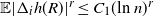 $\mathbb{E}| \Delta_i h(R)|^r \leq C_1 (\text{ln}\ n)^r$
, for
$\mathbb{E}| \Delta_i h(R)|^r \leq C_1 (\text{ln}\ n)^r$
, for
 $ C_1 > 0$
depending on the parameters of the model and r. The first part of Proposition 2.2 is established.
$ C_1 > 0$
depending on the parameters of the model and r. The first part of Proposition 2.2 is established.
For the upper bound on the central moments of f(X), recall the following generalizations of the Efron–Stein inequality (see [Reference Houdré and Ma12, Reference Rhee and Talagrand16]): for
 $r \geq 2$
,
$r \geq 2$
,
 \begin{align}\notag \big(\mathbb{E}|h(R) - \mathbb{E}h(R)|^r\big)^{1/r} \leq \frac{r - 1}{2^{1/r}} \left( \sum_{i = 0}^{|R|-1} \big(\mathbb{E}| h(R) - h\big(R^i\big)|^r \big)^{2/r}\right)^{1/2},\end{align}
and for
 $ r \in (0,2)$
,
$ r \in (0,2)$
,
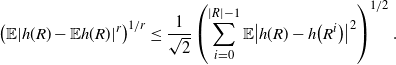 \begin{align}\notag \big(\mathbb{E}|h(R) - \mathbb{E}h(R)|^r\big)^{1/r} \leq \frac{1}{\sqrt{2}} \left( \sum_{i = 0}^{|R|-1} \mathbb{E}\big| h(R) - h\big(R^i\big)\big|^2 \right)^{1/2}.\end{align}
Then, for all
 $r > 0$
,
$r > 0$
,
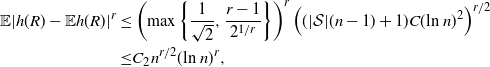 \begin{align}\notag \mathbb{E}|h(R) - \mathbb{E}h(R)|^r \leq & \left( \max \left\{\frac{1}{\sqrt{2}}, \frac{r-1}{2^{1/r}} \right\} \right)^r \left( ( |\mathcal{S}| (n-1) +1 ) C (\text{ln}\ n)^2 \right)^{r/2} \\\notag \leq & C_2 n^{r/2} (\text{ln}\ n)^r,\end{align}
where
 $C_2>0$
is a function of
$C_2>0$
is a function of
 $|\mathcal{S}|$
and r.
$|\mathcal{S}|$
and r.
Remark 5.1. (i) Recall that in the independent setting, there is a single stack, or equivalently, the state space of the latent chain consists of a single element. Then for s as defined in the first paragraph of the above proof,
 $\mathbb{P}(s > 1) = 0$
. Thus we can take
$\mathbb{P}(s > 1) = 0$
. Thus we can take
 $tK = 2$
, and since
$tK = 2$
, and since
 $\mathbb{P}(E_t ) \leq \mathbb{P}(s \geq tk) = 0$
, (33) becomes
$\mathbb{P}(E_t ) \leq \mathbb{P}(s \geq tk) = 0$
, (33) becomes
 \begin{align}\notag \mathbb{E} |h(R) - h\big(R^i\big)|^r \leq (2c)^r,\end{align}
which recovers the independent case.
(ii) Note that the bound on the central moments also follows from using an exponential bounded difference inequality for Markov chains proved by Paulin [Reference Paulin15]. This holds for the general case when X is a Markov chain (not necessarily time-homogeneous) taking values in a Polish space
 $\Lambda = \Lambda_1 \times \cdots \times \Lambda_n$
, with mixing time
$\Lambda = \Lambda_1 \times \cdots \times \Lambda_n$
, with mixing time
 $\tau_{min}$
. Then, for any
$\tau_{min}$
. Then, for any
 $ t \geq 0$
,
$ t \geq 0$
,
 \begin{align}\notag \mathbb{P}( | f(X) - \mathbb{E} [f(X)] | \geq t) \leq 2 \exp \left( \frac{- 2t^2}{||c^*||^2 \tau_{min}} \right),\end{align}
where f is such that
 \begin{align}\notag |f(x) - f(y)| \leq \sum_{i =1}^n c_i \mathbf{1}_{x_i \neq y_i},\end{align}
for any
 $x, y \in \mathbb{R}^n$
and some
$x, y \in \mathbb{R}^n$
and some
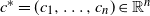 $c^* = (c_1, \ldots, c_n) \in \mathbb{R}^n$
, and where
$c^* = (c_1, \ldots, c_n) \in \mathbb{R}^n$
, and where
 $||c^*||^2 = \sum_{i = 1}^n c_i^2$
.
$||c^*||^2 = \sum_{i = 1}^n c_i^2$
.
5.2. Proof of Proposition 2.3
In this section we no longer require the underlying function f to be Lipschitz.
Let
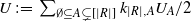 $U \,{:}\,{\raise-1.5pt{=}}\, \sum_{ \emptyset \subseteq A \subsetneq[|R|]} k_{|R|, A} U_A /2$
for a general family of square-integrable random variables
$U \,{:}\,{\raise-1.5pt{=}}\, \sum_{ \emptyset \subseteq A \subsetneq[|R|]} k_{|R|, A} U_A /2$
for a general family of square-integrable random variables
 $U_A(R, R^{\prime})$
. From [Reference Chatterjee2, Lemma 4.4],
$U_A(R, R^{\prime})$
. From [Reference Chatterjee2, Lemma 4.4],
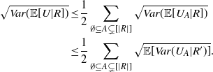 \begin{align}\notag \sqrt{Var(\mathbb{E}[U|R])} \leq & \frac{1}{2} \sum_{\emptyset \subseteq A \subsetneq[|R|]} \sqrt{Var(\mathbb{E}[ U_A | R])} \\\notag \leq & \frac{1}{2} \sum_{\emptyset \subseteq A \subsetneq[|R|]} \sqrt{\mathbb{E}[ Var(U_A | R^{\prime})]}.\end{align}
As in [Reference Lachièze-Rey and Peccati14], this inequality will be used for both
 $U_A = T_A(h)$
and
$U_A = T_A(h)$
and
 $U_A = T^{\prime}_A (h)$
. A major difference from the setting in [Reference Lachièze-Rey and Peccati14, Section 5] is that the function h is not symmetric; i.e., if
$U_A = T^{\prime}_A (h)$
. A major difference from the setting in [Reference Lachièze-Rey and Peccati14, Section 5] is that the function h is not symmetric; i.e., if
 $\sigma$
is a permutation of
$\sigma$
is a permutation of
 $\{ 0, \ldots, |\mathcal{S}|(n-1)\}$
, it is not necessarily the case that
$\{ 0, \ldots, |\mathcal{S}|(n-1)\}$
, it is not necessarily the case that
 $h\big(R_0, \ldots, R_{|\mathcal{S}|(n-1)}\big) = h\big(R_{\sigma(0)}, \ldots, R_{\sigma(|R|(n-1))}\big)$
. Indeed, each variable in R is associated with a transition at a particular step and from a particular state. Fix
$h\big(R_0, \ldots, R_{|\mathcal{S}|(n-1)}\big) = h\big(R_{\sigma(0)}, \ldots, R_{\sigma(|R|(n-1))}\big)$
. Indeed, each variable in R is associated with a transition at a particular step and from a particular state. Fix
 $A \subsetneq[|R|]$
and let
$A \subsetneq[|R|]$
and let
 $\tilde{R}$
be another independent copy of R. Introduce the substitution operator
$\tilde{R}$
be another independent copy of R. Introduce the substitution operator
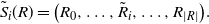 \begin{align}\notag \tilde{S}_i(R) = \big(R_0, \ldots, \tilde{R}_i, \ldots, R_{|R|}\big).\end{align}
Recall that from the Efron–Stein inequality,
 \begin{align}\notag Var\big( U_A | R^{\prime}\big) \leq \frac{1}{2} \sum_{i = 0}^{|R|-1} \mathbb{E}\big[ \big( \tilde{\Delta}_i U_A(R) \big)^2 | R^{\prime}\big],\end{align}
where
 $\tilde{\Delta}_i U_A(R) = U_A\big(\tilde{S}_i(R)\big) - U_A(R)$
.
$\tilde{\Delta}_i U_A(R) = U_A\big(\tilde{S}_i(R)\big) - U_A(R)$
.
Then,
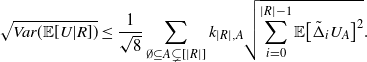 \begin{align} \sqrt{Var( \mathbb{E}[ U| R] )} \leq \frac{1}{\sqrt{8}} \sum_{\emptyset \subseteq A \subsetneq [|R|]} k_{|R|, A} \sqrt{\sum_{i = 0}^{|R| -1} \mathbb{E}\big[ \tilde{\Delta}_i U_A\big]^2}.\end{align}
Recall also that
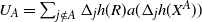 $U_A = \sum_{j \notin A} \Delta_j h(R) a (\Delta_j h(X^A))$
, where the function a is either the identity, or
$U_A = \sum_{j \notin A} \Delta_j h(R) a (\Delta_j h(X^A))$
, where the function a is either the identity, or
 $a ({\cdot}) = | \cdot |$
. Then
$a ({\cdot}) = | \cdot |$
. Then
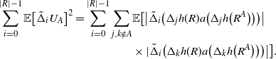 \begin{align}\notag \sum_{i = 0}^{|R| -1} \mathbb{E} \big[ \tilde{\Delta}_i U_A\big]^2 = \sum_{i = 0}^{|R| - 1} \sum_{j, k \notin A} & \mathbb{E} \big[\big| \tilde{\Delta}_i \big( \Delta_j h(R) a \big(\Delta_j h\big(R^A\big)\big)\big)\big| \\ & \times |\tilde{\Delta}_i \big( \Delta_k h(R) a\big(\Delta_k h\big(R^A\big)\big) \big) \big|\big].\end{align}
Fix
 $0 \leq i \leq |R| - 1$
, and note that for
$0 \leq i \leq |R| - 1$
, and note that for
 $j \notin A$
,
$j \notin A$
,
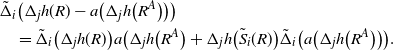 \begin{align}\notag & \tilde{\Delta}_i \big( \Delta_j h(R) - a\big( \Delta_j h\big(R^A\big)\big) \big) \\ & \quad = \tilde{\Delta}_i \big(\Delta_j h(R)\big) a\big(\Delta_j h\big(R^A\big) + \Delta_j h\big(\tilde{S}_i(R)\big) \tilde{\Delta}_i\big(a \big(\Delta_j h\big(R^A\big)\big)\big).\end{align}
Then, using
 $|\tilde{\Delta}_i a({\cdot}) | \leq |\tilde{\Delta}_i ({\cdot})|$
, the summands in (37) are bounded by
$|\tilde{\Delta}_i a({\cdot}) | \leq |\tilde{\Delta}_i ({\cdot})|$
, the summands in (37) are bounded by
 \begin{align} 4 \sup_{Y, Y^{\prime}, Z, Z^{\prime} } \mathbb{E} |\tilde{\Delta}_i \big({\Delta}_j h(Y) \big) {\Delta}_j h\big(Y^{\prime}\big) \tilde{\Delta}_i \big({\Delta}_k h(Z) \big) {\Delta}_k h\big(Z^{\prime}\big)\big|,\end{align}
where Y, Y
′, Z, Z
′ are recombinations of
 $R, R^{\prime}, \tilde{R}$
; i.e.,
$R, R^{\prime}, \tilde{R}$
; i.e.,
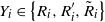 $Y_i \in \big\{R_i, R^{\prime}_i, \tilde{R}_i\big\}$
, for
$Y_i \in \big\{R_i, R^{\prime}_i, \tilde{R}_i\big\}$
, for
 $i \in [0, |R| -1]$
.
$i \in [0, |R| -1]$
.
Next, as in [Reference Lachièze-Rey and Peccati14], we bound each type of summand appearing in (37).
If
 $i = j = k$
, and using
$i = j = k$
, and using
 $\tilde{\Delta}_i \big(\Delta_i ({\cdot})\big) = \Delta_i ({\cdot})$
, (39) is bounded by
$\tilde{\Delta}_i \big(\Delta_i ({\cdot})\big) = \Delta_i ({\cdot})$
, (39) is bounded by
 \begin{align}\notag 4 \sup_{Y, Y^{\prime}, Z, Z^{\prime} } \mathbb{E} | \Delta_i h(Y) \Delta_i h\big(Y^{\prime}\big) \Delta_i h(Z) \Delta_i h\big(Z^{\prime}\big)| \leq 4 \mathbb{E} |\Delta_i h(R)|^4.\end{align}
If
 $i \neq j \neq k$
, we can switch
$i \neq j \neq k$
, we can switch
 $\tilde{R}_i$
and
$\tilde{R}_i$
and
 $R^{\prime}_i $
, and Y is still a recombination. Then (39) is equal to
$R^{\prime}_i $
, and Y is still a recombination. Then (39) is equal to
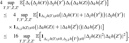 \begin{align}\notag 4 & \sup_{Y, Y^{\prime}, Z, Z^{\prime} } \mathbb{E}\big[ {\Delta}_i \big({\Delta}_j h(Y) \big) {\Delta}_j h\big(Y^{\prime}\big) {\Delta}_i \big({\Delta}_k h(Z) \big) {\Delta}_k h\big(Z^{\prime}\big)\big] \\\notag & \leq \quad 4 \sup_{Y, Y^{\prime}, Z, Z^{\prime}} \mathbb{E}\big[ \mathbf{1}_{\Delta_{i,j} h(Y) \neq 0} \big( | \Delta_j h(Y) | + |\Delta_j h\big(Y^i\big)| \big) | \Delta_j h\big(Y^{\prime}\big) | \\\notag & \quad \times \mathbf{1}_{\Delta_{i,k} h(Z) \neq 0} \big( | \Delta_k h(Z) | + | \Delta_k h\big(Z^i\big) | \big) |\Delta_k h\big(Z^{\prime}\big)|\big] \\ & \leq \quad 16 \sup_{Y, Y^{\prime}, Z, Z^{\prime}} \mathbb{E} \Big[\mathbf{1}_{\Delta_{i,j} h(Y) \neq 0, \Delta_{j,k} h\big(Y^{\prime}\big) \neq 0} |\Delta_j h(Z)|^2 |\Delta_k h\big(Z^{\prime}\big)|^2\Big],\end{align}
where the last step follows from the Cauchy–Schwarz inequality.
If
 $i \neq j = k$
, (39) is equal to
$i \neq j = k$
, (39) is equal to
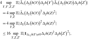 \begin{align}\notag 4 & \sup_{Y, Y^{\prime}, Z, Z^{\prime}} \mathbb{E} | \tilde{\Delta}_i \big(\Delta_j \big(h(Y)\big) \Delta_j h\big(Y^{\prime}\big) \tilde{\Delta}_i \big(\Delta_j \big(h(Z)\big) \Delta_j h\big(Z^{\prime}\big)| \\\notag & = 4 \sup_{Y, Z} \mathbb{E} | \tilde{\Delta}_i \big(\Delta_j \big(h(Y)\big)^2 \Delta_j h(Z)^2 | \\\notag & = 4 \sup_{Y, Z} \mathbb{E} | \Delta_j \big(\Delta_i \big(h(Y)\big)^2 \Delta_j h(Z)^2| \\ & \leq 16 \sup_{Y, Z, Z^{\prime}} \mathbb{E} | \mathbf{1}_{\Delta_{i,j} h(Y) \neq 0} \Delta_i h(Z)^2 \Delta_j h\big(Z^{\prime}\big)^2|,\end{align}
where we have exchanged
 $\tilde{R}_i$
and
$\tilde{R}_i$
and
 $R^{\prime}_i$
and used the Cauchy–Schwarz inequality as in (40).
$R^{\prime}_i$
and used the Cauchy–Schwarz inequality as in (40).
Similarly, if
 $i = j \neq k$
, the bound is
$i = j \neq k$
, the bound is
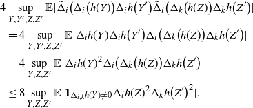 \begin{align}\notag 4 & \sup_{Y, Y^{\prime}, Z, Z^{\prime}} \mathbb{E} | \tilde{\Delta}_i \big(\Delta_i \big(h(Y)\big) \Delta_i h\big(Y^{\prime}\big) \tilde{\Delta}_i \big(\Delta_k \big(h(Z)\big) \Delta_k h\big(Z^{\prime}\big)| \\\notag & = 4 \sup_{Y, Y^{\prime}, Z, Z^{\prime}} \mathbb{E} | \Delta_i h(Y) \Delta_i h\big(Y^{\prime}\big) \Delta_i \big(\Delta_k \big(h(Z)\big) \Delta_k h\big(Z^{\prime}\big) |\\\notag & = 4 \sup_{Y, Z, Z^{\prime}} \mathbb{E} | \Delta_i h(Y)^2 \Delta_i \big(\Delta_k \big(h(Z)\big) \Delta_k h\big(Z^{\prime}\big) |\\ & \leq 8 \sup_{Y, Z, Z^{\prime}} \mathbb{E} | \mathbf{1}_{\Delta_{i,k} h(Y) \neq 0} \Delta_i h(Z)^2 \Delta_k h\big(Z^{\prime}\big)^2|.\end{align}
Finally, if
 $i = k \neq j$
, the bound is by symmetry
$i = k \neq j$
, the bound is by symmetry
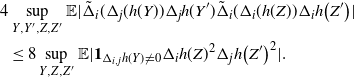 \begin{align}\notag 4 & \sup_{Y, Y^{\prime}, Z, Z^{\prime}} \mathbb{E} | \tilde{\Delta}_i (\Delta_j (h(Y)) \Delta_j h(Y^{\prime}) \tilde{\Delta}_i (\Delta_i (h(Z)) \Delta_i h\big(Z^{\prime}\big)| \\ & \leq 8 \sup_{Y, Z, Z^{\prime}} \mathbb{E} | \mathbf{1}_{\Delta_{i,j} h(Y) \neq 0} \Delta_i h(Z)^2 \Delta_j h\big(Z^{\prime}\big)^2|.\end{align}
Combining (40), (41), (42), and (43) in (37), we finally get
 \begin{align}\notag & \sum_{i = 0}^{|R| -1} \mathbb{E} \big[ \tilde{\Delta}_i U_A\big]^2 \\\notag & \leq 16 \sum_{i = 0}^{|R| -1} \sum_{j, k \notin A}\bigg( \mathbf{1}_{i = j = k} \mathbb{E} |\Delta_i h(R)|^4 + \mathbf{1}_{i \neq j \neq k} B_{|R|}(h) \\\notag & \quad \quad + \big(\mathbf{1}_{i \neq j = k} +\mathbf{1}_{i = k \neq j} \big) B_{|R|}^{(k)}(h) + \big(\mathbf{1}_{i \neq j = k} + \mathbf{1}_{i = j \neq k} \big) B_{|R|}^{(j)}(h) \bigg),\end{align}
where
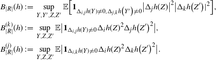 \begin{align}\notag B_{|R|}(h) & \,{:}\,{\raise-1.5pt{=}}\, \sup_{Y, Y^{\prime}, Z, Z^{\prime}} \mathbb{E} \Big[\mathbf{1}_{\Delta_{i,j} h(Y) \neq 0, \Delta_{j,k} h\big(Y^{\prime}\big) \neq 0} \big|\Delta_j h(Z)\big|^2 \big|\Delta_k h\big(Z^{\prime}\big)|^2\Big],\\\notag B_{|R|}^{(k)}(h) & \,{:}\,{\raise-1.5pt{=}}\, \sup_{Y, Z, Z^{\prime}} \mathbb{E} \big| \mathbf{1}_{\Delta_{i,j} h(Y) \neq 0} \Delta_i h(Z)^2 \Delta_j h\big(Z^{\prime}\big)^2\big|, \\\notag B_{|R|}^{(j)} (h) & \,{:}\,{\raise-1.5pt{=}}\, \sup_{Y, Z, Z^{\prime}} \mathbb{E} \big| \mathbf{1}_{\Delta_{i,k} h(Y) \neq 0} \Delta_i h(Z)^2 \Delta_k h\big(Z^{\prime}\big)^2\big|.\end{align}
This suffices for the proof of Proposition 2.3.
Remark 5.2. As observed in [Reference Chu, Shao and Zhang6], the terms involving
 $\Delta_i h(R)$
in (4) and (5) can be removed, leaving only the variance terms. Here is a different way to establish this fact for the particular framework we consider in Section 3. Recall that the expressions on the right-hand sides of (4) and (5) are bounds on terms of the form
$\Delta_i h(R)$
in (4) and (5) can be removed, leaving only the variance terms. Here is a different way to establish this fact for the particular framework we consider in Section 3. Recall that the expressions on the right-hand sides of (4) and (5) are bounds on terms of the form
 \begin{equation*}\mathbb{E}\big| g^{\prime}_t (W) - g^{\prime}_t (W) T\big| + \big|\mathbb{E} \big[g_t(W) W - g^{\prime}_t (W) T\big] \big|,\end{equation*}
where
 $|g^{\prime}_t | \leq 1$
and
$|g^{\prime}_t | \leq 1$
and
 $|g_t(W)W - g^{\prime}_t (W)| = |\mathbf{1}_{W \leq t} - \mathbb{P}(\mathcal{N} \leq t)| \leq 1$
(see [Reference Lachièze-Rey and Peccati14] and [Reference Chatterjee3]). First, note that
$|g_t(W)W - g^{\prime}_t (W)| = |\mathbf{1}_{W \leq t} - \mathbb{P}(\mathcal{N} \leq t)| \leq 1$
(see [Reference Lachièze-Rey and Peccati14] and [Reference Chatterjee3]). First, note that
 \begin{align}\notag \big|g^{\prime}_t(W) - g^{\prime}_t(W)T \big| \geq \big|g^{\prime}_t(W) T \big| - 1\end{align}
and
 \begin{align}\notag 1 \geq \big|g_t(W)W - g^{\prime}_t(W)\big| \geq \big|g_t(W) W\big| - 1.\end{align}
Then, by the triangle inequality and the above,
 \begin{align}\notag \big|g_t(W) W - g^{\prime}_t(W) T\big| \leq \big|g_t(W) W\big| + \big|g^{\prime}_t(W) T\big| \leq \big|g^{\prime}_t(W) - g^{\prime}_t(W)T \big| + 3.\end{align}
Let
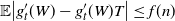 $\mathbb{E} \big| g^{\prime}_t(W) - g^{\prime}_t(W) T\big| \leq f(n)$
for some function f, with
$\mathbb{E} \big| g^{\prime}_t(W) - g^{\prime}_t(W) T\big| \leq f(n)$
for some function f, with
 $f(n) \to \infty$
and such that for
$f(n) \to \infty$
and such that for
 $\sigma^2 = \sigma^2(n)$
,
$\sigma^2 = \sigma^2(n)$
,
 $f(n) / \sigma^2 \to 0$
. Then
$f(n) / \sigma^2 \to 0$
. Then
 \begin{align}\notag \big| \mathbb{E}\big[ g_t(W)W - g^{\prime}_t(W)T\big]| / \sigma^3 \leq C f(n) / \sigma^2,\end{align}
for some constant
 $C > 0$
that does not depend on n. Therefore, the asymptotic behavior of the bounds in (4) and (5) is given by the terms corresponding to
$C > 0$
that does not depend on n. Therefore, the asymptotic behavior of the bounds in (4) and (5) is given by the terms corresponding to
 $\mathbb{E} | g^{\prime}_t(W) - g^{\prime}_t(W)T|$
, i.e., the terms involving the variance. This modification of the method is also valid in our framework and would ‘improve’ our results. However, it does not have a significant effect on the rates obtained in our applications in Section 3, and so we will not pursue it any further here.
$\mathbb{E} | g^{\prime}_t(W) - g^{\prime}_t(W)T|$
, i.e., the terms involving the variance. This modification of the method is also valid in our framework and would ‘improve’ our results. However, it does not have a significant effect on the rates obtained in our applications in Section 3, and so we will not pursue it any further here.
5.3. Proof of Proposition 3.1
Recall that
 \begin{align} B_{|R|}(h) & \,{:}\,{\raise-1.5pt{=}}\, \sup_{Y, Y^{\prime}, Z, Z^{\prime}} \mathbb{E} \Big[\mathbf{1}_{\Delta_{i,j} h(Y) \neq 0, \Delta_{j,k} h\big(Y^{\prime}\big) \neq 0} |\Delta_j h(Z)|^2 |\Delta_k h\big(Z^{\prime}\big)|^2\Big],\end{align}
where the supremum is taken over recombinations of R and its independent copies R ′ and R ′′.
Let E be the event that at least one of the perturbations of the instructions in (44) yields a difference in more than K points. By Proposition 5.1, there is
 $\epsilon > 0$
such that
$\epsilon > 0$
such that
 $\mathbb{P}( E) \leq (1 - \epsilon)^K$
. Then, by the Lipschitz property of h,
$\mathbb{P}( E) \leq (1 - \epsilon)^K$
. Then, by the Lipschitz property of h,
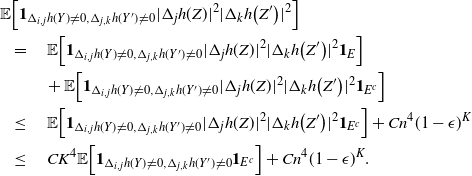 \begin{align}\notag \mathbb{E} & \Big[\mathbf{1}_{\Delta_{i,j} h(Y) \neq 0, \Delta_{j,k} h(Y^{\prime}) \neq 0} |\Delta_j h(Z)|^2 |\Delta_k h\big(Z^{\prime}\big)|^2\Big] \\\notag & = \quad \mathbb{E} \Big[\mathbf{1}_{\Delta_{i,j} h(Y) \neq 0, \Delta_{j,k} h(Y^{\prime}) \neq 0} |\Delta_j h(Z)|^2 |\Delta_k h\big(Z^{\prime}\big)|^2 \mathbf{1}_{E}\Big] \\\notag & \quad \quad + \mathbb{E} \Big[\mathbf{1}_{\Delta_{i,j} h(Y) \neq 0, \Delta_{j,k} h(Y^{\prime}) \neq 0} |\Delta_j h(Z)|^2 |\Delta_k h\big(Z^{\prime}\big)|^2 \mathbf{1}_{E^c}\Big] \\\notag & \leq \quad \mathbb{E} \Big[\mathbf{1}_{\Delta_{i,j} h(Y) \neq 0, \Delta_{j,k} h(Y^{\prime}) \neq 0} |\Delta_j h(Z)|^2 |\Delta_k h\big(Z^{\prime}\big)|^2 \mathbf{1}_{E^c}\Big] + Cn^4 (1- \epsilon)^K \\ & \leq \quad CK^4 \mathbb{E} \Big[ \mathbf{1}_{\Delta_{i,j} h(Y) \neq 0, \Delta_{j,k} h(Y^{\prime}) \neq 0} \mathbf{1}_{E^c}\Big] + Cn^4 (1- \epsilon)^K.\end{align}
If S(Y) is the set of points generated by the instructions Y and
 $S(Y^i)$
—the set of points generated by Y after the perturbation of
$S(Y^i)$
—the set of points generated by Y after the perturbation of
 $Y_i$
—let
$Y_i$
—let
 \begin{align}\notag S_1 \,{:}\,{\raise-1.5pt{=}}\, & S(Y) \Delta S\big(Y^i\big),\end{align}
where
 $\Delta$
is the symmetric difference operator. Similarly, let
$\Delta$
is the symmetric difference operator. Similarly, let
 \begin{align}\notag S_2 \,{:}\,{\raise-1.5pt{=}}\, & S(Y) \Delta S\big(Y^j\big), \\\notag S_3 \,{:}\,{\raise-1.5pt{=}}\, & S(Y^{\prime}) \Delta S\big(\big(Y^{\prime}\big)^i\big), \\\notag S_4 \,{:}\,{\raise-1.5pt{=}}\, & S(Y^{\prime}) \Delta S\big(\big(Y^{\prime}\big)^j\big).\end{align}
Note that, conditioned on
 $E^c$
,
$E^c$
,
 $|S_i| \leq 2K$
for
$|S_i| \leq 2K$
for
 $i = 1, 2,3, 4$
. Furthermore, if
$i = 1, 2,3, 4$
. Furthermore, if
 $s_1 \cap s_2 = \emptyset$
for all
$s_1 \cap s_2 = \emptyset$
for all
 $(s_1, s_2) \in (S_1, S_2)$
, then
$(s_1, s_2) \in (S_1, S_2)$
, then
 $\Delta_{i, j} h(Y) = 0$
. Then
$\Delta_{i, j} h(Y) = 0$
. Then
 \begin{align}\notag \mathbf{1}_{\Delta_{i,j} h(Y)} \leq \sum_{(s_1, s_2) \in (S_1, S_2) } \mathbf{1}_{s_1 \cap s_2 \neq \emptyset}.\end{align}
This bound is meaningful if the sets
 $S_1$
and
$S_1$
and
 $S_2$
are disjoint sets of random variables. Conditioned on
$S_2$
are disjoint sets of random variables. Conditioned on
 $E^c$
, this is the case if
$E^c$
, this is the case if
 $|i - j| \geq |\mathcal{S}|K$
. We introduce events
$|i - j| \geq |\mathcal{S}|K$
. We introduce events
 $E_1$
,
$E_1$
,
 $E_2$
, and
$E_2$
, and
 $E_3$
corresponding to 0, 1, or 2 of the conditions
$E_3$
corresponding to 0, 1, or 2 of the conditions
 $\{ |i - j| \geq |\mathcal{S}| K, |j- k| \geq |\mathcal{S}| K\}$
holding, respectively. The events
$\{ |i - j| \geq |\mathcal{S}| K, |j- k| \geq |\mathcal{S}| K\}$
holding, respectively. The events
 $E_1$
,
$E_1$
,
 $E_2,$
and
$E_2,$
and
 $E_3$
are deterministic. Then we have
$E_3$
are deterministic. Then we have
 \begin{align}\notag \mathbb{E}& \big[ \mathbf{1}_{\Delta_{i,j} h(Y) \neq 0, \Delta_{j,k} h(Y^{\prime}) \neq 0} \mathbf{1}_{E^c}\big] = \mathbb{E} \Big[ \mathbf{1}_{\Delta_{i,j} h(Y) \neq 0, \Delta_{j,k} h(Y^{\prime}) \neq 0} \mathbf{1}_{E^c} \big( \mathbf{1}_{E_1} + \mathbf{1}_{E_2} + \mathbf{1}_{E_3}\big)\Big].\end{align}
First we use the trivial bound
 $\mathbf{1}_{\Delta_{i,j} h(Y) \neq 0, \Delta_{j,k} h(Y^{\prime}) \neq 0} \leq 1$
to get
$\mathbf{1}_{\Delta_{i,j} h(Y) \neq 0, \Delta_{j,k} h(Y^{\prime}) \neq 0} \leq 1$
to get
 \begin{align} \mathbb{E}& \Big[ \mathbf{1}_{\Delta_{i,j} h(Y) \neq 0, \Delta_{j,k} h(Y^{\prime}) \neq 0} \mathbf{1}_{E^c} \mathbf{1}_{E_1} \Big] \leq \mathbf{1}_{E_1}.\end{align}
Then, for the term with
 $\mathbf{1}_{E_3}$
,
$\mathbf{1}_{E_3}$
,
 \begin{align}\notag \mathbb{E}& \Big[ \mathbf{1}_{\Delta_{i,j} h(Y) \neq 0, \Delta_{j,k} h(Y^{\prime}) \neq 0} \mathbf{1}_{E^c} \mathbf{1}_{E_3} \Big] \leq \mathbf{1}_{E_3} \mathbb{E} \left[ \sum_{(s_1, s_2) \in (S_1, S_2) } \sum_{(s_3, s_4) \in (S_3, S_4) } \mathbf{1}_{s_1 \cap s_2 \neq \emptyset, s_3 \cap s_4 \neq \emptyset}\right].\end{align}
To bound
 $\mathbb{E} \big[ \mathbf{1}_{s_1 \cap s_2 \neq \emptyset, s_3 \cap s_4 \neq \emptyset}\big]$
, we condition on
$\mathbb{E} \big[ \mathbf{1}_{s_1 \cap s_2 \neq \emptyset, s_3 \cap s_4 \neq \emptyset}\big]$
, we condition on
 $s_2$
,
$s_2$
,
 $s_3$
, and the values of all hidden variables H. Then, since
$s_3$
, and the values of all hidden variables H. Then, since
 $S_1$
and
$S_1$
and
 $S_4$
are disjoint, we have independence:
$S_4$
are disjoint, we have independence:
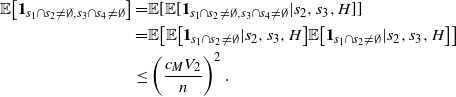 \begin{align}\notag \mathbb{E} \big[ \mathbf{1}_{s_1 \cap s_2 \neq \emptyset, s_3 \cap s_4 \neq \emptyset}\big] = & \mathbb{E} [ \mathbb{E} [ \mathbf{1}_{s_1 \cap s_2 \neq \emptyset, s_3 \cap s_4 \neq \emptyset} | s_2, s_3, H]] \\\notag = & \mathbb{E} \big[ \mathbb{E} \big[ \mathbf{1}_{s_1 \cap s_2 \neq \emptyset} |s_2, s_3, H\big] \mathbb{E} \big[ \mathbf{1}_{s_1 \cap s_2 \neq \emptyset} | s_2, s_3, H\big] \big] \\\notag \leq & \left(\frac{c_M V_2}{n}\right)^2.\end{align}
Therefore,
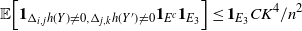 \begin{align} \mathbb{E}& \Big[ \mathbf{1}_{\Delta_{i,j} h(Y) \neq 0, \Delta_{j,k} h(Y^{\prime}) \neq 0} \mathbf{1}_{E^c} \mathbf{1}_{E_3} \Big] \leq \mathbf{1}_{E_3} C K^4/n^2\end{align}
for some
 $C > 0$
independent of K and n, where we have used that
$C > 0$
independent of K and n, where we have used that
 $|S_i| \leq 2K$
for
$|S_i| \leq 2K$
for
 $i = 1,2,3,4$
.
$i = 1,2,3,4$
.
Finally, for the term with
 $E_2$
, we may assume that
$E_2$
, we may assume that
 $|i - j| \geq |\mathcal{S}|K$
, since the case
$|i - j| \geq |\mathcal{S}|K$
, since the case
 $|j - k| \geq |\mathcal{S}|K$
is identical. Write, using the trivial bound on
$|j - k| \geq |\mathcal{S}|K$
is identical. Write, using the trivial bound on
 $\mathbf{1}_{\Delta_{j,k} h(Y^{\prime})} \neq 0$
,
$\mathbf{1}_{\Delta_{j,k} h(Y^{\prime})} \neq 0$
,
 \begin{align}\notag \mathbb{E}& \big[ \mathbf{1}_{\Delta_{i,j} h(Y) \neq 0, \Delta_{j,k} h(Y^{\prime}) \neq 0} \mathbf{1}_{E^c} \mathbf{1}_{E_2} \big] \leq \mathbf{1}_{E_3} \mathbb{E} \left[ \sum_{(s_1, s_2) \in (S_1, S_2) } \mathbf{1}_{s_1 \cap s_2 \neq \emptyset}\right].\end{align}
Next, as before,
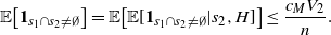 \begin{align}\notag \mathbb{E} \big[ \mathbf{1}_{s_1 \cap s_2 \neq \emptyset}\big] = \mathbb{E}\big[ \mathbb{E} [ \mathbf{1}_{s_1 \cap s_2 \neq \emptyset} | s_2, H]\big] \leq \frac{c_M V_2}{n}.\end{align}
Then
 \begin{align} \mathbb{E}& \big[ \mathbf{1}_{\Delta_{i,j} h(Y) \neq 0, \Delta_{j,k} h(Y^{\prime}) \neq 0} \mathbf{1}_{E^c} \mathbf{1}_{E_2} \big] \leq \mathbf{1}_{E_2} C K^2/n.\end{align}
Combining (45), (46), (48), and (47), we get the following bound on (44):
 \begin{align}\notag B_{|R|}(h) \leq C\Big( \mathbf{1}_{E_1} K^4 + \mathbf{1}_{E_2} K^6/n + \mathbf{1}_{E_3} K^8/n^2 + n^4 (1 - \epsilon)^K\Big).\end{align}
Then,
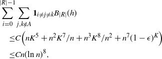 \begin{align}\notag \sum_{i = 0}^{|R| -1} & \sum_{j, k \notin A} \mathbf{1}_{i \neq j \neq k} B_{|R|}(h) \\\notag \leq & C\Big( n K^5 + n^2 K^7 /n + n^3 K^8 /n^2 + n^7 (1 - \epsilon)^K \Big) \\\notag \leq & Cn (\text{ln}\ n)^8,\end{align}
when we choose
 $K = c \text{ln}\ n$
for a suitable
$K = c \text{ln}\ n$
for a suitable
 $ c> 0$
, independent of n.
$ c> 0$
, independent of n.
5.4. Proof of Proposition 3.2
As in the proof of Proposition 5.1, the sequence of instructions
 $R^i$
may give rise to a different realization (Z
′, X
′). Indeed, if the instruction
$R^i$
may give rise to a different realization (Z
′, X
′). Indeed, if the instruction
 $R_i$
determines
$R_i$
determines
 $\big(Z_j, X_j\big)$
and
$\big(Z_j, X_j\big)$
and
 $R^{\prime}_i $
determines
$R^{\prime}_i $
determines
 $\big(Z^{\prime}_j, X^{\prime}_j\big)$
, it is possible that
$\big(Z^{\prime}_j, X^{\prime}_j\big)$
, it is possible that
 $\big(Z_j, X_j\big) \neq \big(Z^{\prime}_j, X^{\prime}_j\big)$
. Let
$\big(Z_j, X_j\big) \neq \big(Z^{\prime}_j, X^{\prime}_j\big)$
. Let
 $s \geq 0$
be the smallest integer (possibly
$s \geq 0$
be the smallest integer (possibly
 $s = \infty$
) such that
$s = \infty$
) such that
 $Z_{j + s} = Z^{\prime}_{j+s} $
. Then, as in (31), there is
$Z_{j + s} = Z^{\prime}_{j+s} $
. Then, as in (31), there is
 $\epsilon > 0$
such that for
$\epsilon > 0$
such that for
 $K \in \mathbb{N}$
,
$K \in \mathbb{N}$
,
 \begin{align}\notag \mathbb{P}(s \geq K) \leq (1 - \epsilon)^K.\end{align}
Fix K, and let E be the event corresponding to
 $\{s \geq K\}$
. Using the trivial bound
$\{s \geq K\}$
. Using the trivial bound
 $|h(R)| \leq n$
, and thus
$|h(R)| \leq n$
, and thus
 $|\Delta_i h(R)| \leq 2n$
, we have
$|\Delta_i h(R)| \leq 2n$
, we have
 \begin{align}\notag \mathbb{E} |\Delta_i h |^t = & \quad \mathbb{E} \big[ |\Delta_i h |^t \mathbf{1}_E\big] + \mathbb{E} \big[|\Delta_i h |^t \mathbf{1}_{E^c} \big] \\ \leq & \quad (2n)^t (1 - \epsilon)^K + \mathbb{E} \big[|\Delta_i h |^t \mathbf{1}_{E^c} \big].\end{align}
Let S(R) be the set of points generated by the sequence of instructions R, and let
 $S(R^j)$
be the points generated by R after the perturbation of
$S(R^j)$
be the points generated by R after the perturbation of
 $R_j$
. Set
$R_j$
. Set
 $S = S(R) \Delta S(R^j)$
for the symmetric difference and
$S = S(R) \Delta S(R^j)$
for the symmetric difference and
 $S^c = S(R) \cap S(R^j)$
. Note that
$S^c = S(R) \cap S(R^j)$
. Note that
 $E^c$
implies that
$E^c$
implies that
 $|\mathcal{S}| \leq 2K$
. Furthermore,
$|\mathcal{S}| \leq 2K$
. Furthermore,
 \begin{align}\notag |\Delta_i h| \leq \sum_{s \in S} \sum_{x \in S^c} \mathbf{1}_{s \cap x \neq \emptyset},\end{align}
and
 \begin{align}\notag |\Delta_i h|^t \leq \sum_{(s_1, \ldots, s_t) \in S^t} \sum_{(x_1, \ldots, x_t) \in (S^c)^t} \prod_{j, \ell = 1}^t \mathbf{1}_{s_j \cap x_{\ell} \neq \emptyset},\end{align}
To estimate (49), we need to evaluate
 \begin{equation*}\mathbb{E}\Bigg[ \prod_{j, \ell = 1}^t \mathbf{1}_{s_j \cap x_{\ell} \neq \emptyset}\Bigg],\end{equation*}
and to do so we proceed as in [Reference Lachièze-Rey and Peccati14] by studying the shape of the relations of
 $(s_j, x_{\ell})_{j, \ell \in \{1, \ldots, t\}}$
.
$(s_j, x_{\ell})_{j, \ell \in \{1, \ldots, t\}}$
.
Identify the set
 $(s_j, x_{\ell})_{j, \ell \in \{1, \ldots, t\}}$
with the edges of the graph G whose vertices correspond to
$(s_j, x_{\ell})_{j, \ell \in \{1, \ldots, t\}}$
with the edges of the graph G whose vertices correspond to
 $(s_j)_{j \in \{1, \ldots, t\}}$
and
$(s_j)_{j \in \{1, \ldots, t\}}$
and
 $(x_{\ell})_{ \ell \in \{1, \ldots, t\}}$
. In particular, if
$(x_{\ell})_{ \ell \in \{1, \ldots, t\}}$
. In particular, if
 $s_{j_1} = s_{j_2}$
for some
$s_{j_1} = s_{j_2}$
for some
 $j_1 \neq j_2$
, we identify them with the same point in the graph G. Conditioned on the realization of the hidden chain Z, we have independence. Then, if G is a tree, fix a root and condition recursively on vertices at different distances from the root. By the restrictions on the volume of the grain and the sampling distribution,
$j_1 \neq j_2$
, we identify them with the same point in the graph G. Conditioned on the realization of the hidden chain Z, we have independence. Then, if G is a tree, fix a root and condition recursively on vertices at different distances from the root. By the restrictions on the volume of the grain and the sampling distribution,
 \begin{align}\notag \mathbb{E}\left[ \prod_{j, \ell = 1}^t \mathbf{1}_{s_j \cap x_{\ell} \neq \emptyset} \bigg| Z = z^n\right] \leq \left(\frac{c_M V_2}{n}\right)^{|E(G)|},\end{align}
where
 $|E(G)|$
is the number of edges in the graph G. Furthermore,
$|E(G)|$
is the number of edges in the graph G. Furthermore,
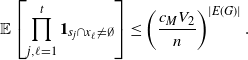 \begin{align}\notag \mathbb{E}\left[ \prod_{j, \ell = 1}^t \mathbf{1}_{s_j \cap x_{\ell} \neq \emptyset} \right] \leq \left(\frac{c_M V_2}{n}\right)^{|E(G)|}.\end{align}
Note that the same result holds if G is a graph without cycles, i.e., a collection of disjoint trees. In general, G might have cycles. Let T be a subgraph of G that contains no cycles. Then
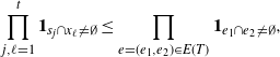 \begin{align}\notag \prod_{j, \ell = 1}^t \mathbf{1}_{s_j \cap x_{\ell} \neq \emptyset} \leq \prod_{e = (e_1,e_2) \in E(T)} \mathbf{1}_{e_1 \cap e_2 \neq \emptyset},\end{align}
where the product on the right-hand side runs over the edges
 $e = (e_1, e_2)$
of the graph T with
$e = (e_1, e_2)$
of the graph T with
 $e_1 \in S$
and
$e_1 \in S$
and
 $e_2 \in S^c$
. Let
$e_2 \in S^c$
. Let
 $|\mathcal{S}|$
be the number of distinct vertices in
$|\mathcal{S}|$
be the number of distinct vertices in
 $(s_1, \ldots, s_t)$
, and similarly let
$(s_1, \ldots, s_t)$
, and similarly let
 $|x|$
be the number for
$|x|$
be the number for
 $(x_1, \ldots, x_t)$
. The graph G is complete bipartite with
$(x_1, \ldots, x_t)$
. The graph G is complete bipartite with
 $|S| + |x|$
vertices. We can find a subgraph T of G, also with
$|S| + |x|$
vertices. We can find a subgraph T of G, also with
 $|S| + |x|$
vertices and no cycles. Then
$|S| + |x|$
vertices and no cycles. Then
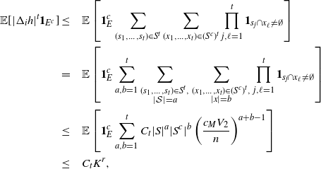 \begin{align}\notag \mathbb{E} [ |\Delta_i h|^t \mathbf{1}_{E^c} ] \leq & \quad \mathbb{E} \left[ \mathbf{1}_E^c \sum_{(s_1, \ldots, s_t) \in S^t} \sum_{(x_1, \ldots, x_t) \in (S^c)^t} \prod_{j, \ell = 1}^t \mathbf{1}_{s_j \cap x_{\ell} \neq \emptyset}\right] \\\notag = & \quad \mathbb{E} \left[ \mathbf{1}_E^c \sum_{a, b = 1}^t \sum_{ \substack{(s_1, \ldots, s_t) \in S^t,\\ |\mathcal{S}| = a}} \sum_{\substack{(x_1, \ldots, x_t) \in (S^c)^t,\\ |x| = b}} \prod_{j, \ell = 1}^t \mathbf{1}_{s_j \cap x_{\ell} \neq \emptyset}\right] \\\notag \leq & \quad \mathbb{E} \left[ \mathbf{1}_E^c \sum_{a, b = 1}^t C_t |S|^a |S^c|^b \left(\frac{c_M V_2}{n}\right)^{a + b -1} \right] \\\notag \leq & \quad C_t K^r,\end{align}
where
 $C_t > 0$
is a constant depending on t, and where we have used that
$C_t > 0$
is a constant depending on t, and where we have used that
 $|\mathcal{S}| \leq 2K$
and
$|\mathcal{S}| \leq 2K$
and
 $|S^c| \leq 2n$
.
$|S^c| \leq 2n$
.
Let
 $K = c\text{ln}\ n$
for a suitable
$K = c\text{ln}\ n$
for a suitable
 $c > 0$
; then (49) implies (15) as desired.
$c > 0$
; then (49) implies (15) as desired.
5.5. Proof of Proposition 3.3
As before, let E be the event that all perturbations of instructions in (44) propagate at most K levels. We have that
 $\mathbb{P}(E^c) \leq (1 - \epsilon)^K$
for some
$\mathbb{P}(E^c) \leq (1 - \epsilon)^K$
for some
 $\epsilon \in (0,1)$
. Using the trivial bound
$\epsilon \in (0,1)$
. Using the trivial bound
 $|h(Y)| \leq n$
,
$|h(Y)| \leq n$
,
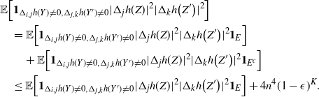 \begin{align}\notag & \mathbb{E} \Big[ \mathbf{1}_{\Delta_{i,j} h(Y) \neq 0,\Delta_{j,k} h(Y^{\prime}) \neq 0} |\Delta_j h(Z)|^2 |\Delta_k h\big(Z^{\prime}\big)|^2 \Big] \\\notag & \quad = \mathbb{E} \Big[ \mathbf{1}_{\Delta_{i,j} h(Y) \neq 0,\Delta_{j,k} h(Y^{\prime}) \neq 0} |\Delta_j h(Z)|^2 |\Delta_k h\big(Z^{\prime}\big)|^2 \mathbf{1}_E\Big] \\\notag & \qquad + \mathbb{E} \Big[ \mathbf{1}_{\Delta_{i,j} h(Y) \neq 0,\Delta_{j,k} h(Y^{\prime}) \neq 0} |\Delta_j h(Z)|^2 |\Delta_k h\big(Z^{\prime}\big)|^2 \mathbf{1}_{E^c}\Big]\\ & \quad \leq \mathbb{E} \Big[ \mathbf{1}_{\Delta_{i,j} h(Y) \neq 0,\Delta_{j,k} h(Y^{\prime}) \neq 0} |\Delta_j h(Z)|^2 |\Delta_k h\big(Z^{\prime}\big)|^2 \mathbf{1}_E\Big] + 4n^4 (1 -\epsilon)^K.\end{align}
Let
 $S(Y^i)$
be the set of points generated by the sequence of instructions Y after the perturbation of
$S(Y^i)$
be the set of points generated by the sequence of instructions Y after the perturbation of
 $Y_i$
. Let S be the set of all points in the expectation above, and furthermore let
$Y_i$
. Let S be the set of all points in the expectation above, and furthermore let
 \begin{align}\notag S_1 \,{:}\,{\raise-1.5pt{=}}\, & S(Y) \Delta S\big(Y^i\big), \quad S_2 \,{:}\,{\raise-1.5pt{=}}\, S(Y) \Delta S\big(Y^j\big), \\\notag S_3 \,{:}\,{\raise-1.5pt{=}}\, & S\big(Y^{\prime}\big) \Delta S\big(\big(Y^{\prime}\big)^j\big), \quad S_4 \,{:}\,{\raise-1.5pt{=}}\, S\big(Y^{\prime}\big) \Delta S\big(\big(Y^{\prime}\big)^k\big), \\\notag S_5 \,{:}\,{\raise-1.5pt{=}}\, & S(Z) \Delta S\big(Z^j \big), \quad S_6 \,{:}\,{\raise-1.5pt{=}}\, S\big(Z^{\prime}\big) \Delta S\big(Z^k\big),\end{align}
where
 $\Delta$
is the symmetric difference operator. Conditioned on E,
$\Delta$
is the symmetric difference operator. Conditioned on E,
 $|S_i| \leq 2K$
for
$|S_i| \leq 2K$
for
 $i = 1, \ldots, 6$
and
$i = 1, \ldots, 6$
and
 $ |\mathcal{S}| \leq 10n$
.
$ |\mathcal{S}| \leq 10n$
.
Conditioned on E, if
 $j - i \leq |\mathcal{S}| K$
, the perturbation in i might be propagating past the position corresponding to the instruction j, leading to difficulties in the analysis of
$j - i \leq |\mathcal{S}| K$
, the perturbation in i might be propagating past the position corresponding to the instruction j, leading to difficulties in the analysis of
 $\Delta_{i,j} h(Y)$
. This is why we condition further on the events
$\Delta_{i,j} h(Y)$
. This is why we condition further on the events
 $E_1, E_2, E_3$
corresponding respectively to 0, 1, or 2 of the conditions
$E_1, E_2, E_3$
corresponding respectively to 0, 1, or 2 of the conditions
 $\{|i - j| \geq |\mathcal{S}|K, |j - k| \geq |\mathcal{S}|K\}$
holding true. Note that
$\{|i - j| \geq |\mathcal{S}|K, |j - k| \geq |\mathcal{S}|K\}$
holding true. Note that
 $E_1$
,
$E_1$
,
 $E_2$
, and
$E_2$
, and
 $E_3$
are deterministic.
$E_3$
are deterministic.
If
 $E_1$
holds, we use the trivial bound
$E_1$
holds, we use the trivial bound
 $ \mathbf{1}_{\Delta_{i,j} h(Y) \neq 0,\Delta_{j,k} h(Y^{\prime}) \neq 0} \leq 1$
, which leads to
$ \mathbf{1}_{\Delta_{i,j} h(Y) \neq 0,\Delta_{j,k} h(Y^{\prime}) \neq 0} \leq 1$
, which leads to
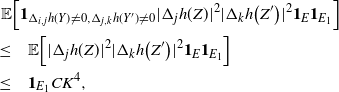 \begin{align}\notag \mathbb{E} & \Big[ \mathbf{1}_{\Delta_{i,j} h(Y) \neq 0,\Delta_{j,k} h(Y^{\prime}) \neq 0} |\Delta_j h(Z)|^2 |\Delta_k h\big(Z^{\prime}\big)|^2 \mathbf{1}_E \mathbf{1}_{E_1}\Big] \\\notag \leq & \quad \mathbb{E} \Big[ |\Delta_j h(Z)|^2 |\Delta_k h\big(Z^{\prime}\big)|^2 \mathbf{1}_E \mathbf{1}_{E_1}\Big] \\ \leq & \quad \mathbf{1}_{E_1} C K^4,\end{align}
using the Cauchy–Schwarz inequality.
Conditioned on
 $E_3$
, the sets
$E_3$
, the sets
 $S_1$
,
$S_1$
,
 $S_2 \cup S_3$
, and
$S_2 \cup S_3$
, and
 $S_4$
are pairwise disjoint. Next, in similarity to an argument presented in [Reference Lachièze-Rey and Peccati14], if
$S_4$
are pairwise disjoint. Next, in similarity to an argument presented in [Reference Lachièze-Rey and Peccati14], if
 $s_1 \cap s = \emptyset$
and
$s_1 \cap s = \emptyset$
and
 $s_2 \cap s = \emptyset$
for all
$s_2 \cap s = \emptyset$
for all
 $(s_1, s_2, s) \in (S_1, S_2, S)$
, then
$(s_1, s_2, s) \in (S_1, S_2, S)$
, then
 $\Delta_{i,j} h(Y) = 0$
. Therefore,
$\Delta_{i,j} h(Y) = 0$
. Therefore,
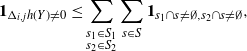 \begin{align}\notag \mathbf{1}_{\Delta_{i,j} h(Y) \neq 0} \leq \sum_{ \substack{ s_1 \in S_1 \\ s_2 \in S_2 } } \sum_{s \in S} \mathbf{1}_{s_1 \cap s \neq \emptyset, s_2 \cap s \neq \emptyset},\end{align}
and also
 \begin{align}\notag \mathbf{1}_{\Delta_{j,k} h(Y^{\prime}) \neq 0} \leq \sum_{\substack{ s_3 \in S_3 \\ s_4 \in S_4} } \sum_{s \in S} \mathbf{1}_{s_3 \cap s \neq \emptyset, s_4 \cap s \neq \emptyset}.\end{align}
Furthermore,
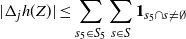 \begin{align}\notag |\Delta_j h(Z) | \leq \sum_{s_5 \in S_5} \sum_{s \in S} \mathbf{1}_{s_5 \cap s \neq \emptyset}\end{align}
and
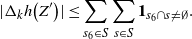 \begin{align}\notag |\Delta_k h\big(Z^{\prime}\big) | \leq \sum_{s_6 \in S} \sum_{s \in S} \mathbf{1}_{s_6 \cap s \neq \emptyset}.\end{align}
Therefore,
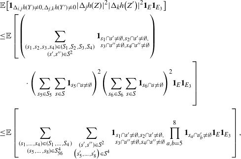 \begin{align}\notag \mathbb{E} & \big[ \mathbf{1}_{\Delta_{i,j} h(Y) \neq 0,\Delta_{j,k} h(Y^{\prime}) \neq 0} |\Delta_j h(Z)|^2 |\Delta_k h\big(Z^{\prime}\big)|^2 \mathbf{1}_E \mathbf{1}_{E_3} \big] \\
\notag \leq & \mathbb{E} \left[ \left( \sum_{ \substack {(s_1, s_2, s_3, s_4) \in (S_1, S_2, S_3, S_4) \\ (s^{\prime}, s^{\prime\prime}) \in S^2} } \mathbf{1}_{\substack{ s_1 \cap s^{\prime} \neq \emptyset, s_2 \cap s^{\prime} \neq \emptyset,\\ s_3 \cap s^{\prime\prime} \neq \emptyset, s_4 \cap s^{\prime\prime} \neq \emptyset}}\right)\right. \\
\notag & \quad \quad \left. \vphantom{\sum_{ \substack {(s_1, s_2, s_3, s_4) \in (S_1, S_2, S_3, S_4) \\ (s^{\prime}, s^{\prime\prime}) \in S^2} }} \cdot \Bigg( \sum_{s_5 \in S_5} \sum_{s \in S} \mathbf{1}_{s_5 \cap s \neq \emptyset}\Bigg)^2 \Bigg( \sum_{s_6 \in S_6} \sum_{s \in S} \mathbf{1}_{s_6 \cap s \neq \emptyset}\Bigg)^2 \mathbf{1}_E \mathbf{1}_{E_3} \right] \\
\leq & \mathbb{E} \left[ \sum_{ \substack {(s_1, \ldots, s_4) \in (S_1, \ldots, S_4) \\ (s_5, \ldots, s_8) \in S_{56}^4 } } \sum_{\substack{ (s^{\prime}, s^{\prime\prime}) \in S^2 \\ \big(s^{\prime}_5, \ldots, s^{\prime}_8\big) \in S^4}} \mathbf{1}_{\substack{ s_1 \cap s^{\prime} \neq \emptyset, s_2 \cap s^{\prime} \neq \emptyset,\\ s_3 \cap s^{\prime\prime} \neq \emptyset, s_4 \cap s^{\prime\prime} \neq \emptyset}} \prod_{a, b = 5}^8 \mathbf{1}_{s_a \cap s^{\prime}_b \neq \emptyset} \mathbf{1}_E \mathbf{1}_{E_3} \right],\end{align}
\begin{align}\notag \mathbb{E} & \big[ \mathbf{1}_{\Delta_{i,j} h(Y) \neq 0,\Delta_{j,k} h(Y^{\prime}) \neq 0} |\Delta_j h(Z)|^2 |\Delta_k h\big(Z^{\prime}\big)|^2 \mathbf{1}_E \mathbf{1}_{E_3} \big] \\
\notag \leq & \mathbb{E} \left[ \left( \sum_{ \substack {(s_1, s_2, s_3, s_4) \in (S_1, S_2, S_3, S_4) \\ (s^{\prime}, s^{\prime\prime}) \in S^2} } \mathbf{1}_{\substack{ s_1 \cap s^{\prime} \neq \emptyset, s_2 \cap s^{\prime} \neq \emptyset,\\ s_3 \cap s^{\prime\prime} \neq \emptyset, s_4 \cap s^{\prime\prime} \neq \emptyset}}\right)\right. \\
\notag & \quad \quad \left. \vphantom{\sum_{ \substack {(s_1, s_2, s_3, s_4) \in (S_1, S_2, S_3, S_4) \\ (s^{\prime}, s^{\prime\prime}) \in S^2} }} \cdot \Bigg( \sum_{s_5 \in S_5} \sum_{s \in S} \mathbf{1}_{s_5 \cap s \neq \emptyset}\Bigg)^2 \Bigg( \sum_{s_6 \in S_6} \sum_{s \in S} \mathbf{1}_{s_6 \cap s \neq \emptyset}\Bigg)^2 \mathbf{1}_E \mathbf{1}_{E_3} \right] \\
\leq & \mathbb{E} \left[ \sum_{ \substack {(s_1, \ldots, s_4) \in (S_1, \ldots, S_4) \\ (s_5, \ldots, s_8) \in S_{56}^4 } } \sum_{\substack{ (s^{\prime}, s^{\prime\prime}) \in S^2 \\ \big(s^{\prime}_5, \ldots, s^{\prime}_8\big) \in S^4}} \mathbf{1}_{\substack{ s_1 \cap s^{\prime} \neq \emptyset, s_2 \cap s^{\prime} \neq \emptyset,\\ s_3 \cap s^{\prime\prime} \neq \emptyset, s_4 \cap s^{\prime\prime} \neq \emptyset}} \prod_{a, b = 5}^8 \mathbf{1}_{s_a \cap s^{\prime}_b \neq \emptyset} \mathbf{1}_E \mathbf{1}_{E_3} \right],\end{align}
where
 $S_{56} = S_5 \cup S_6$
and
$S_{56} = S_5 \cup S_6$
and
 $|S_{56}| \leq 4K$
, conditioned on E.
$|S_{56}| \leq 4K$
, conditioned on E.
To evaluate the summand expression we use the graph representation. Let
 $E_{\ell}$
be the event that there are
$E_{\ell}$
be the event that there are
 $\ell$
distinct points among
$\ell$
distinct points among
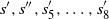 $s^{\prime},s^{\prime\prime}, s^{\prime}_5, \ldots, s^{\prime}_8$
, different from
$s^{\prime},s^{\prime\prime}, s^{\prime}_5, \ldots, s^{\prime}_8$
, different from
 $s_1, \ldots, s_8$
. Note that
$s_1, \ldots, s_8$
. Note that
 $\ell \in [0, 6]$
. Conditioned on
$\ell \in [0, 6]$
. Conditioned on
 $E_{\ell}$
, we can find a subgraph with no cycles and
$E_{\ell}$
, we can find a subgraph with no cycles and
 $\ell + 2$
edges, of the graph with edges
$\ell + 2$
edges, of the graph with edges
 $\{ \{s_1, s^{\prime}\}, \{s_2, s^{\prime}\}, \{s_3, s^{\prime\prime}\}, \{s_4, s^{\prime\prime}\} \} \cup \{ \big\{s_a, s^{\prime}_b \big\}\,:\, a, b \in [5,8]\}$
. Indeed, note that there are at least 3 different points among
$\{ \{s_1, s^{\prime}\}, \{s_2, s^{\prime}\}, \{s_3, s^{\prime\prime}\}, \{s_4, s^{\prime\prime}\} \} \cup \{ \big\{s_a, s^{\prime}_b \big\}\,:\, a, b \in [5,8]\}$
. Indeed, note that there are at least 3 different points among
 $s_1, \ldots, s_4$
. Next, if there are x points present among s
′, s
′′ and
$s_1, \ldots, s_4$
. Next, if there are x points present among s
′, s
′′ and
 $\ell - x$
points among
$\ell - x$
points among
 $s^{\prime}_5, \ldots, s^{\prime}_8 $
, we can find a subgraph with no cycles with at least
$s^{\prime}_5, \ldots, s^{\prime}_8 $
, we can find a subgraph with no cycles with at least
 $\ell - x$
edges among
$\ell - x$
edges among
 $\{ \big\{s_a, s^{\prime}_b \big\}\,:\, a, b \in [5,8]\}$
and
$\{ \big\{s_a, s^{\prime}_b \big\}\,:\, a, b \in [5,8]\}$
and
 $x + 2$
edges among
$x + 2$
edges among
 $\{ \{s_1, s^{\prime}\}, \{s_2, s^{\prime}\}, \{s_3, s^{\prime\prime}\}, \{s_4, s^{\prime\prime}\} \}$
.
$\{ \{s_1, s^{\prime}\}, \{s_2, s^{\prime}\}, \{s_3, s^{\prime\prime}\}, \{s_4, s^{\prime\prime}\} \}$
.
Then, if we further condition on the values of the hidden variables H, we get, by independence,
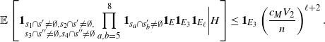 \begin{align}\notag \mathbb{E} \left[ \mathbf{1}_{\substack{ s_1 \cap s^{\prime} \neq \emptyset, s_2 \cap s^{\prime} \neq \emptyset,\\ s_3 \cap s^{\prime\prime} \neq \emptyset, s_4 \cap s^{\prime\prime} \neq \emptyset}} \prod_{a, b = 5}^8 \mathbf{1}_{s_a \cap s^{\prime}_b \neq \emptyset} \mathbf{1}_E \mathbf{1}_{E_3} \mathbf{1}_{E_{\ell}} \bigg| H\right] \leq \mathbf{1}_{E_3} \left( \frac{c_M V_2}{n}\right)^{\ell + 2}.\end{align}
Then (52) is further bounded by
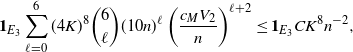 \begin{align} \mathbf{1}_{E_3} \sum_{\ell = 0}^6 (4K)^8 \binom{6}{\ell} (10n)^{\ell} \left( \frac{c_M V_2}{n}\right)^{\ell + 2} \leq \mathbf{1}_{E_3} C K^8 n^{-2},\end{align}
for some
 $C > 0$
independent of n and K.
$C > 0$
independent of n and K.
Finally, assume that
 $E_2$
holds and that
$E_2$
holds and that
 $|i - j| \geq |\mathcal{S}| K$
. The case
$|i - j| \geq |\mathcal{S}| K$
. The case
 $|j - k| \geq |\mathcal{S}|K$
is identical. As above, using the trivial bound
$|j - k| \geq |\mathcal{S}|K$
is identical. As above, using the trivial bound
 $\mathbf{1}_{\Delta_{j,k} h(Y^{\prime}) \neq 0} \leq 1$
,
$\mathbf{1}_{\Delta_{j,k} h(Y^{\prime}) \neq 0} \leq 1$
,
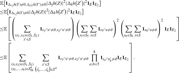 \begin{align}\notag \mathbb{E} & \big[ \mathbf{1}_{\Delta_{i,j} h(Y) \neq 0,\Delta_{j,k} h(Y^{\prime}) \neq 0} |\Delta_j h(Z)|^2 |\Delta_k h\big(Z^{\prime}\big)|^2 \mathbf{1}_E \mathbf{1}_{E_2} \big] \\
\notag \leq & \mathbb{E} \big[ \mathbf{1}_{\Delta_{i,j} h(Y) \neq 0} |\Delta_j h(Z)|^2 |\Delta_k h\big(Z^{\prime}\big)|^2 \mathbf{1}_E \mathbf{1}_{E_2} \big] \\
\notag \leq & \mathbb{E} \left[ \left( \sum_{ \substack {(s_1, s_2) \in (S_1, S_2) \\ s^{\prime} \in S} } \mathbf{1}_{ s_1 \cap s^{\prime} \neq \emptyset, s_2 \cap s^{\prime} \neq \emptyset}\right) \left( \sum_{s_5 \in S_5} \sum_{s \in S} \mathbf{1}_{s_5 \cap s \neq \emptyset}\right)^2 \left( \sum_{s_6 \in S_6} \sum_{s \in S} \mathbf{1}_{s_6 \cap s \neq \emptyset}\right)^2 \mathbf{1}_E \mathbf{1}_{E_2} \right] \\
\leq & \mathbb{E} \left[ \sum_{ \substack {(s_1 s_2) \in (S_1, S_2) \\ (s_5, \ldots, s_8) \in S_{56}^4 } } \sum_{\substack{ s^{\prime} \in S \\ \big(s^{\prime}_5, \ldots, s^{\prime}_8\big) \in S^4}} \mathbf{1}_{ s_1 \cap s^{\prime} \neq \emptyset, s_2 \cap s^{\prime} \neq \emptyset} \prod_{a, b = 5}^8 \mathbf{1}_{s_a \cap s^{\prime}_b \neq \emptyset} \mathbf{1}_E \mathbf{1}_{E_2} \right].\end{align}
\begin{align}\notag \mathbb{E} & \big[ \mathbf{1}_{\Delta_{i,j} h(Y) \neq 0,\Delta_{j,k} h(Y^{\prime}) \neq 0} |\Delta_j h(Z)|^2 |\Delta_k h\big(Z^{\prime}\big)|^2 \mathbf{1}_E \mathbf{1}_{E_2} \big] \\
\notag \leq & \mathbb{E} \big[ \mathbf{1}_{\Delta_{i,j} h(Y) \neq 0} |\Delta_j h(Z)|^2 |\Delta_k h\big(Z^{\prime}\big)|^2 \mathbf{1}_E \mathbf{1}_{E_2} \big] \\
\notag \leq & \mathbb{E} \left[ \left( \sum_{ \substack {(s_1, s_2) \in (S_1, S_2) \\ s^{\prime} \in S} } \mathbf{1}_{ s_1 \cap s^{\prime} \neq \emptyset, s_2 \cap s^{\prime} \neq \emptyset}\right) \left( \sum_{s_5 \in S_5} \sum_{s \in S} \mathbf{1}_{s_5 \cap s \neq \emptyset}\right)^2 \left( \sum_{s_6 \in S_6} \sum_{s \in S} \mathbf{1}_{s_6 \cap s \neq \emptyset}\right)^2 \mathbf{1}_E \mathbf{1}_{E_2} \right] \\
\leq & \mathbb{E} \left[ \sum_{ \substack {(s_1 s_2) \in (S_1, S_2) \\ (s_5, \ldots, s_8) \in S_{56}^4 } } \sum_{\substack{ s^{\prime} \in S \\ \big(s^{\prime}_5, \ldots, s^{\prime}_8\big) \in S^4}} \mathbf{1}_{ s_1 \cap s^{\prime} \neq \emptyset, s_2 \cap s^{\prime} \neq \emptyset} \prod_{a, b = 5}^8 \mathbf{1}_{s_a \cap s^{\prime}_b \neq \emptyset} \mathbf{1}_E \mathbf{1}_{E_2} \right].\end{align}
If we condition on
 $E_{\ell}$
and the values of the hidden variables H, we get
$E_{\ell}$
and the values of the hidden variables H, we get
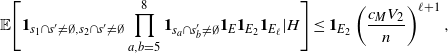 \begin{align}\notag \mathbb{E} \Bigg[ \mathbf{1}_{ s_1 \cap s^{\prime} \neq \emptyset, s_2 \cap s^{\prime} \neq \emptyset} \prod_{a, b = 5}^8 \mathbf{1}_{s_a \cap s^{\prime}_b \neq \emptyset} \mathbf{1}_E \mathbf{1}_{E_2} \mathbf{1}_{E_{\ell}} | H \Bigg] \leq \mathbf{1}_{E_2} \left( \frac{c_M V_2}{n}\right)^{\ell + 1},\end{align}
since in this case
 $s_1$
and
$s_1$
and
 $s_2$
are distinct and we can find a subgraph with
$s_2$
are distinct and we can find a subgraph with
 $\ell + 1$
edges and no cycles.
$\ell + 1$
edges and no cycles.
Then (54) is bounded by
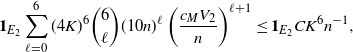 \begin{align} \mathbf{1}_{E_2} \sum_{\ell = 0}^6 (4K)^6 \binom{6}{\ell} (10n)^{\ell} \left( \frac{c_M V_2}{n}\right)^{\ell + 1} \leq \mathbf{1}_{E_2} C K^6 n^{-1},\end{align}
for some
 $C > 0$
.
$C > 0$
.
We get the following bound on
 $B_{|R|} (h)$
using (50), (51), (55), and (53):
$B_{|R|} (h)$
using (50), (51), (55), and (53):
 \begin{align}\notag B_{|R|}(h) \leq C \Big( \mathbf{1}_{E_1} K^4 + \mathbf{1}_{E_2} K^6 /n + \mathbf{1}_{E_3} K^8 / n^2 + n^4 (1 - \epsilon)^K\Big).\end{align}
Then,
 \begin{align}\notag \sum_{i = 0}^{|R| - 1} & \sum_{j, k \notin A} \mathbf{1}_{i \neq j \neq k} B_{|R|} (h) \\\notag \leq & C \Big( n K^6 + n^2 K^7/n + n^3 K^8 /n^2 + n^7 (1 - \epsilon)^K\Big) \\\notag \leq & C n (\text{ln}\ n)^8,\end{align}
where we have chosen
 $K = c \text{ln}\ n$
for a suitable
$K = c \text{ln}\ n$
for a suitable
 $c > 0$
, independent of n.
$c > 0$
, independent of n.
5.6. Proof of Lemma 4.1
To simplify computations, we introduce the process X ′ defined as
 \begin{align}\notag X^{\prime} = \bigcup_{m \in \mathbb{Z}^d} (X + m).\end{align}
Unlike in the independent setting in [Reference Lachièze-Rey and Peccati14], here the law of X
′ is invariant only under integer-valued translations. Note that, almost surely, X
′ has exactly n points in any cube
 $[t, t+1]^d$
, where
$[t, t+1]^d$
, where
 $t \in \mathbb{R}$
. Let
$t \in \mathbb{R}$
. Let
 $T_x = \big\{ [y, y+1]^d \,:\, y \in \mathbb{R}^d, x \in [y, y+1]^d\big\}$
. Define
$T_x = \big\{ [y, y+1]^d \,:\, y \in \mathbb{R}^d, x \in [y, y+1]^d\big\}$
. Define
 $\overline{R_k}(x;\, X)$
as
$\overline{R_k}(x;\, X)$
as
 \begin{align}\notag \overline{R_k}(x;\, X) \,{:}\,{\raise-1.5pt{=}}\, \sup_{T \in T_x} R_k (x;\, X^{\prime} \cap T).\end{align}
Note that if
 $x \in [0,1]^d$
, then
$x \in [0,1]^d$
, then
 $[0,1 ]^d \in T_x$
and so
$[0,1 ]^d \in T_x$
and so
 $\overline{R_k}(x;\, X^{\prime}) \geq R_k(x;\, X)$
. When the
$\overline{R_k}(x;\, X^{\prime}) \geq R_k(x;\, X)$
. When the
 $X_i$
are sampled independently and uniformly, as in [Reference Lachièze-Rey and Peccati14], it is the case that
$X_i$
are sampled independently and uniformly, as in [Reference Lachièze-Rey and Peccati14], it is the case that
 $\overline{R_k}(x;\, X^{\prime})$
does not depend on the position of x. However, in the hidden Markov model case we need to find a further bound on
$\overline{R_k}(x;\, X^{\prime})$
does not depend on the position of x. However, in the hidden Markov model case we need to find a further bound on
 $\overline{R_k}(x;\, X^{\prime})$
.
$\overline{R_k}(x;\, X^{\prime})$
.
For that purpose, consider the cube
 $K_0 \,{:}\,{\raise-1.5pt{=}}\, [-1/2, 1/2]^d$
of volume 1 centered at
$K_0 \,{:}\,{\raise-1.5pt{=}}\, [-1/2, 1/2]^d$
of volume 1 centered at
 $\mathbf{0} \in \mathbb{R}^d$
. Let
$\mathbf{0} \in \mathbb{R}^d$
. Let
 $B_A$
be the open ball of
$B_A$
be the open ball of
 $\mathbb{R}^d$
centered at
$\mathbb{R}^d$
centered at
 $\mathbf{0}$
and of volume
$\mathbf{0}$
and of volume
 $A < 1$
, to be chosen later. Next, let
$A < 1$
, to be chosen later. Next, let
 $\tilde{X} = \big(0, \tilde{X}_1, \ldots, \tilde{X}_{n-1}\big)$
be such that
$\tilde{X} = \big(0, \tilde{X}_1, \ldots, \tilde{X}_{n-1}\big)$
be such that
 $\tilde{X}_i \in K_0$
for all
$\tilde{X}_i \in K_0$
for all
 $i = 1, \ldots, n-1$
. Furthermore, for any Lebesgue-measurable
$i = 1, \ldots, n-1$
. Furthermore, for any Lebesgue-measurable
 $T \subseteq K_0$
, set
$T \subseteq K_0$
, set
 \begin{align}\notag \mathbb{P}\big(\tilde{X}_i \in T\big) = c_m |T \cap B_A| + c_M |T \cap B_A^c|\end{align}
for all
 $i \in 1, \ldots, n-1$
, where
$i \in 1, \ldots, n-1$
, where
 $|\cdot|$
now denotes the Lebesgue measure of the corresponding sets. If
$|\cdot|$
now denotes the Lebesgue measure of the corresponding sets. If
 $A = (c_M - 1)/(c_M - c_m)$
, then the above is a well-defined positive measure on
$A = (c_M - 1)/(c_M - c_m)$
, then the above is a well-defined positive measure on
 $K_0$
. From the restrictions of the hidden Markov model, if
$K_0$
. From the restrictions of the hidden Markov model, if
 $\tilde{R}_k = R_k(0;\, \tilde{X})$
,
$\tilde{R}_k = R_k(0;\, \tilde{X})$
,
 \begin{align}\notag \overline{R_k}(x;\, X) \leq \tilde{R}_k.\end{align}
Indeed,
 $\tilde{R}_k$
represents the worst-case scenario where the remaining points of X are least likely to be distributed in the volume closest to x.
$\tilde{R}_k$
represents the worst-case scenario where the remaining points of X are least likely to be distributed in the volume closest to x.
Then,
 \begin{align} \mathbb{E} U_k^q(i) \leq \mathbb{E}_{X_i, \tilde{X}}\Big[ \mathbf{1}_{d(X_i;\, \partial K) \leq \tilde{R}_k} \tilde{R}_k^{qd}\Big] \leq S_+(K) \mathbb{E}_{\tilde{X}}\Big[\tilde{R}_k^{qd+ \alpha}\Big],\end{align}
where we have used the upper bound on
 $Vol(\partial K^r)$
.
$Vol(\partial K^r)$
.
To estimate
 $\mathbb{E}\big[ \tilde{R}_k^{qd+ \alpha}\big]$
, note that if
$\mathbb{E}\big[ \tilde{R}_k^{qd+ \alpha}\big]$
, note that if
 $\tilde{R}_k \geq r$
, there will be an open ball of radius
$\tilde{R}_k \geq r$
, there will be an open ball of radius
 $r/2k$
in
$r/2k$
in
 $K_0$
containing no points of
$K_0$
containing no points of
 $\tilde{X}$
. Moreover, there will be
$\tilde{X}$
. Moreover, there will be
 $s_d \in (0,1)$
, depending only on the dimension d, such that every ball of radius 2k contains a cube of side length
$s_d \in (0,1)$
, depending only on the dimension d, such that every ball of radius 2k contains a cube of side length
 $s_d r/k$
of the form
$s_d r/k$
of the form
 $[g - s_d r/ 2k, g + s_d r/ 2k]$
, where
$[g - s_d r/ 2k, g + s_d r/ 2k]$
, where
 $g \in (s_d r / k) \mathbb{Z}^d $
. Then, if
$g \in (s_d r / k) \mathbb{Z}^d $
. Then, if
 $s_d r / k < 1$
,
$s_d r / k < 1$
,
 \begin{align}\notag \mathbb{P} (\tilde{R}_k \geq r) \leq & \mathbb{P} ( \exists g \in (s_d r / k ) \mathbb{Z}^d \,:\, \tilde{X} \cap \big[g - s_d r/ 2k, g + s_d r/ 2k\big] = \mathbf{0}) \\\notag \leq & \# \big\{ g \,:\, g \in (s_d r / k) \mathbb{Z}^d \cap [-r, r]^d\big\} \mathbb{P}( \tilde{X} \cap \big[ - s_d r/ 2k, s_d r/ 2k\big] = \mathbf{0}) \\\notag \leq & \frac{k^d}{(s_d )^d} \big(1 - c_m (s_d r / k)^d\big)^{n-1}.\end{align}
If, on the other hand,
 $s_d r / k \geq 1$
, then
$s_d r / k \geq 1$
, then
 $ \tilde{X} \cap [g - s_d r/ 2k, g + s_d r/ 2k] = \tilde{X}$
and
$ \tilde{X} \cap [g - s_d r/ 2k, g + s_d r/ 2k] = \tilde{X}$
and
 $ \mathbb{P}\big(\tilde{R}_k \geq r\big) = 0$
. Using
$ \mathbb{P}\big(\tilde{R}_k \geq r\big) = 0$
. Using
 $1 - x \leq e^{-x}$
, for any
$1 - x \leq e^{-x}$
, for any
 $u > 0$
we have
$u > 0$
we have
 \begin{align}\notag \mathbb{E}\big[ \tilde{R}(0, \tilde{X})^u \big] = & \int_0^{\infty} \mathbb{P}\big( \tilde{R}(0, \tilde{X}) \geq r^{1/u}\big) dr \\\notag \leq & c_{d, k} \int_0^{\infty} \Big(1 - c_m \big(s_d r^{1/u} / k\big)^d\Big)^{n-1} dr \\\notag \leq & c_{d, k} \int_0^{\infty} \exp\Big( - c_m (n-1) \big(s_d r^{1/u} / k\big)^{d}\Big) dr \\\notag \leq & c_{d, k, u} (n-1)^{u/d} \int_0^{\infty} \exp \big(-r^{d/u}\big) dr.\end{align}
Applying the above in (56) yields
 \begin{align}\notag \mathbb{E} U_k^q(i) \leq c_{d, k, qd + \alpha} S_+(K) n^{- q- \alpha/ d},\end{align}
where
 $c_{d, k, qd + \alpha} > 0$
depends only on the parameters of the transition probabilities of the hidden chain and on d, k, and
$c_{d, k, qd + \alpha} > 0$
depends only on the parameters of the transition probabilities of the hidden chain and on d, k, and
 $qd + \alpha$
, but neither on n nor on i.
$qd + \alpha$
, but neither on n nor on i.
5.7. Proof of Proposition 4.5
We analyze
 \begin{align} B_{|R|} (h) \,{:}\,{\raise-1.5pt{=}}\, \sup_{Y, Y^{\prime}, Z, Z^{\prime}} \mathbb{E}\big[ \mathbf{1}_{\Delta_{i,j} h(Y) \neq 0} \mathbf{1}_{\Delta_{j,k} h(Y^{\prime}) \neq 0} |\Delta_j h(Z)|^2 |\Delta_k h\big(Z^{\prime}\big)|^2 \big],\end{align}
where as before the supremum is taken over recombinations Y, Y
′, Z, Z
′ of R, R
′, R
′′. Let E be the event that all perturbations of the instructions in (57) propagate at most T levels. There is
 $\epsilon > 0$
, depending only on the parameters of the models, such that
$\epsilon > 0$
, depending only on the parameters of the models, such that
 $\mathbb{P}(E^c) \leq (1 - \epsilon)^T$
.
$\mathbb{P}(E^c) \leq (1 - \epsilon)^T$
.
As before, conditioned on E, if
 $|j - i| \leq |\mathcal{S}| K$
, the perturbation in i might be propagating past the position corresponding to the instruction j, leading to difficulties in the analysis of
$|j - i| \leq |\mathcal{S}| K$
, the perturbation in i might be propagating past the position corresponding to the instruction j, leading to difficulties in the analysis of
 $\Delta_{i,j} h(Y)$
. This is the reason for conditioning further on the events
$\Delta_{i,j} h(Y)$
. This is the reason for conditioning further on the events
 $E_1, E_2, E_3$
corresponding respectively to 0, 1, or 2 of the conditions
$E_1, E_2, E_3$
corresponding respectively to 0, 1, or 2 of the conditions
 $\{|i - j| \geq |\mathcal{S}|K, |j - k| \geq |\mathcal{S}|K\}$
holding. Note that
$\{|i - j| \geq |\mathcal{S}|K, |j - k| \geq |\mathcal{S}|K\}$
holding. Note that
 $E_1$
,
$E_1$
,
 $E_2$
, and
$E_2$
, and
 $E_3$
are deterministic.
$E_3$
are deterministic.
In this setting, we also study the event that all Voronoi cells are small. For that purpose, as in [Reference Lachièze-Rey and Peccati14], we introduce the event
 $\Omega_n(X)$
, given by
$\Omega_n(X)$
, given by
 \begin{align}\notag \Omega_n (X) \,{:}\,{\raise-1.5pt{=}}\, \left( \max_{1 \leq j \leq n} R\big(X_j;\, X\big) \leq n^{-1/d} \rho_n \right),\end{align}
where
 $\rho_n = (\text{ln}\ n)^{1/d + \epsilon^{\prime}}$
for
$\rho_n = (\text{ln}\ n)^{1/d + \epsilon^{\prime}}$
for
 $\epsilon^{\prime}$
sufficiently small. Then, after conditioning on the realization of the hidden chain, a proof as in [Reference Lachièze-Rey and Peccati14, Lemma 6.8] leads to
$\epsilon^{\prime}$
sufficiently small. Then, after conditioning on the realization of the hidden chain, a proof as in [Reference Lachièze-Rey and Peccati14, Lemma 6.8] leads to
 \begin{align} n^{\eta} ( 1 - \mathbb{P}(\Omega_n (X))) \to 0\end{align}
as
 $n \to \infty$
, for all
$n \to \infty$
, for all
 $\eta > 0$
.
$\eta > 0$
.
We now estimate
 $B_{|R|}(h)$
. Write
$B_{|R|}(h)$
. Write
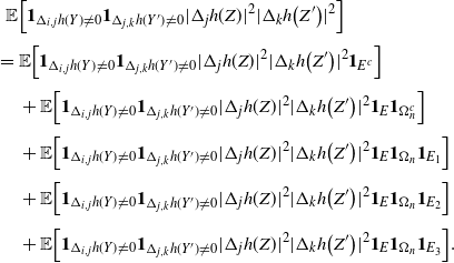 \begin{align}\notag \mathbb{E} & \Big[ \mathbf{1}_{\Delta_{i,j} h(Y) \neq 0} \mathbf{1}_{\Delta_{j,k} h(Y^{\prime}) \neq 0} |\Delta_j h(Z)|^2 |\Delta_k h\big(Z^{\prime}\big)|^2 \Big] \\[3pt]\notag =\, & \mathbb{E} \Big[ \mathbf{1}_{\Delta_{i,j} h(Y) \neq 0} \mathbf{1}_{\Delta_{j,k} h(Y^{\prime}) \neq 0} |\Delta_j h(Z)|^2 |\Delta_k h\big(Z^{\prime}\big)|^2 \mathbf{1}_{E^c}\Big] \\[3pt]\notag & + \mathbb{E} \Big[ \mathbf{1}_{\Delta_{i,j} h(Y) \neq 0} \mathbf{1}_{\Delta_{j,k} h(Y^{\prime}) \neq 0} |\Delta_j h(Z)|^2 |\Delta_k h\big(Z^{\prime}\big)|^2 \mathbf{1}_{E} \mathbf{1}_{\Omega_n^c}\Big] \\[3pt]\notag & + \mathbb{E} \Big[ \mathbf{1}_{\Delta_{i,j} h(Y) \neq 0} \mathbf{1}_{\Delta_{j,k} h(Y^{\prime}) \neq 0} |\Delta_j h(Z)|^2 |\Delta_k h\big(Z^{\prime}\big)|^2 \mathbf{1}_{E} \mathbf{1}_{\Omega_n} \mathbf{1}_{E_1}\Big]\\[3pt]\notag & + \mathbb{E} \Big[ \mathbf{1}_{\Delta_{i,j} h(Y) \neq 0} \mathbf{1}_{\Delta_{j,k} h(Y^{\prime}) \neq 0} |\Delta_j h(Z)|^2 |\Delta_k h\big(Z^{\prime}\big)|^2 \mathbf{1}_{E} \mathbf{1}_{\Omega_n} \mathbf{1}_{E_2}\Big]\\[3pt] & + \mathbb{E} \Big[ \mathbf{1}_{\Delta_{i,j} h(Y) \neq 0} \mathbf{1}_{\Delta_{j,k} h(Y^{\prime}) \neq 0} |\Delta_j h(Z)|^2 |\Delta_k h\big(Z^{\prime}\big)|^2 \mathbf{1}_{E} \mathbf{1}_{\Omega_n} \mathbf{1}_{E_3}\Big].\end{align}
Using
 $|\Delta_j h(Z)|, |\Delta_k h\big(Z^{\prime}\big)| \leq 1$
, we get that the first two terms in (59) are bounded by
$|\Delta_j h(Z)|, |\Delta_k h\big(Z^{\prime}\big)| \leq 1$
, we get that the first two terms in (59) are bounded by
 $\mathbb{P}(E^c) +\mathbb{P}(\Omega_n^c)$
. Next,
$\mathbb{P}(E^c) +\mathbb{P}(\Omega_n^c)$
. Next,
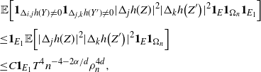 \begin{align}\notag \mathbb{E} & \Big[ \mathbf{1}_{\Delta_{i,j} h(Y) \neq 0} \mathbf{1}_{\Delta_{j,k} h(Y^{\prime}) \neq 0} |\Delta_j h(Z)|^2 |\Delta_k h\big(Z^{\prime}\big)|^2 \mathbf{1}_{E} \mathbf{1}_{\Omega_n} \mathbf{1}_{E_1}\Big] && \\[3pt]\notag \leq & \mathbf{1}_{E_1} \mathbb{E} \Big[ |\Delta_j h(Z)|^2 |\Delta_k h\big(Z^{\prime}\big)|^2 \mathbf{1}_{E} \mathbf{1}_{\Omega_n}\Big] &&\\[3pt] \leq & C \mathbf{1}_{E_1} T^4 n^{-4 - 2 \alpha/d} \rho_n^{4d}, &&\end{align}
where we have used the Cauchy–Schwarz inequality.
Next, define as before
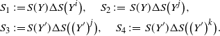 \begin{align}\notag S_1 \,{:}\,{\raise-1.5pt{=}}\, & S(Y) \Delta S\big(Y^i\big), \quad S_2 \,{:}\,{\raise-1.5pt{=}}\, S(Y) \Delta S\big(Y^j\big), \\\notag S_3 \,{:}\,{\raise-1.5pt{=}}\, & S(Y^{\prime}) \Delta S\big(\big(Y^{\prime}\big)^j\big), \quad S_4 \,{:}\,{\raise-1.5pt{=}}\, S(Y^{\prime}) \Delta S\big(\big(Y^{\prime}\big)^k\big).\end{align}
Further, let
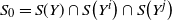 $S_0 = S(Y) \cap S\big(Y^i\big) \cap S\big(Y^j\big)$
and
$S_0 = S(Y) \cap S\big(Y^i\big) \cap S\big(Y^j\big)$
and
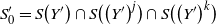 $S^{\prime}_0 = S\big(Y^{\prime}\big) \cap S\big(\big(Y^{\prime}\big)^j\big) \cap S\big(\big(Y^{\prime}\big)^k\big)$
. By Proposition 4.4(ii), it follows that conditioned on
$S^{\prime}_0 = S\big(Y^{\prime}\big) \cap S\big(\big(Y^{\prime}\big)^j\big) \cap S\big(\big(Y^{\prime}\big)^k\big)$
. By Proposition 4.4(ii), it follows that conditioned on
 $\Omega_n$
,
$\Omega_n$
,
 \begin{align}\notag \mathbf{1}_{\Delta_{i,j} h(Y) \neq 0} \leq & \sum_{s_1 \in S_1, s_2 \in S_2} \mathbf{1}_{d_{S_0}(s_1, \partial K) \leq 2n^{-1/d} \rho_n } \mathbf{1}_{d_{S_0}(s_2, \partial K) \leq 2n^{-1/d} \rho_n } \mathbf{1}_{d_{S_0}(s_1, s_2) \leq 2n^{-1/d} \rho_n}.\end{align}
Conditioned on
 $E_3$
, the sets
$E_3$
, the sets
 $S_1$
,
$S_1$
,
 $S_2 \cup S_3$
, and
$S_2 \cup S_3$
, and
 $S_4$
are pairwise disjoint:
$S_4$
are pairwise disjoint:
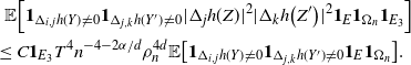 \begin{align}\notag \mathbb{E} & \Big[ \mathbf{1}_{\Delta_{i,j} h(Y) \neq 0} \mathbf{1}_{\Delta_{j,k} h(Y^{\prime}) \neq 0} |\Delta_j h(Z)|^2 |\Delta_k h\big(Z^{\prime}\big)|^2 \mathbf{1}_{E} \mathbf{1}_{\Omega_n} \mathbf{1}_{E_3}\Big] &&\\\notag \leq\, & C \mathbf{1}_{E_3} T^4 n^{-4 - 2 \alpha/d} \rho_n^{4d} \mathbb{E} \big[ \mathbf{1}_{\Delta_{i,j} h(Y) \neq 0} \mathbf{1}_{\Delta_{j,k} h(Y^{\prime}) \neq 0} \mathbf{1}_{E} \mathbf{1}_{\Omega_n}\big].&&\end{align}
By conditioning on the realization of all hidden chains H, we obtain
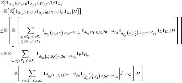 \begin{align}\notag \mathbb{E} & \big[ \mathbf{1}_{\Delta_{i,j} h(Y) \neq 0} \mathbf{1}_{\Delta_{j,k} h(Y^{\prime}) \neq 0} \mathbf{1}_{E} \mathbf{1}_{\Omega_n}\big] \\\notag = & \mathbb{E}\big[ \mathbb{E} \big[ \mathbf{1}_{\Delta_{i,j} h(Y) \neq 0} \mathbf{1}_{\Delta_{j,k} h(Y^{\prime}) \neq 0} \mathbf{1}_{E} \mathbf{1}_{\Omega_n} | H\big]\big] \\\notag \leq & \mathbb{E} \left[ \mathbb{E}\left[ \sum_{ \substack{ s_1 \in S_1, s_2 \in S_2 \\ s^{\prime}_1 \in S_3, s^{\prime}_2 \in S_4}} \mathbf{1}_{d_{S_0}\big(s^{\prime}_1, \partial K\big) \leq 2n^{-1/d} \rho_n } \mathbf{1}_{d_{S_0}(s_1, s_2) \leq 2n^{-1/d} \rho_n} \mathbf{1}_{d_{S^{\prime}_0}\big(s^{\prime}_1, s^{\prime}_2\big) \leq 2n^{-1/d} \rho_n} \mathbf{1}_{E} \mathbf{1}_{\Omega_n} | H \right] \right] \\ \notag \leq & \mathbb{E} \mathbb{E} \Bigg[ \sum_{ s_2 \in S_2, s^{\prime}_1 \in S_1} \mathbf{1}_{d_{S_0}\big(s^{\prime}_1, \partial K\big) \leq 2n^{-1/d} \rho_n } \mathbf{1}_{E} \mathbf{1}_{\Omega_n} \\ \notag & \quad \quad \mathbb{E} \Bigg[ \sum_{ s_1 \in S_1, s^{\prime}_2 \in S_4} \mathbf{1}_{d_{S_0}(s_1, s_2) \leq 2n^{-1/d} \rho_n} \mathbf{1}_{d_{S^{\prime}_0}\big(s^{\prime}_1, s^{\prime}_2\big) \leq 2n^{-1/d} \rho_n} \bigg| s^{\prime}_1, s_2\Bigg] \bigg| H \Bigg].\end{align}
Now, conditioned on H,
 $s^{\prime}_1$
, and
$s^{\prime}_1$
, and
 $s_2$
, we have independence in the innermost expectation. Therefore, the above is bounded by
$s_2$
, we have independence in the innermost expectation. Therefore, the above is bounded by
 \begin{align}\notag \mathbb{E} \Bigg[ \sum_{ s_2 \in S_2, s^{\prime}_1 \in S_1} \mathbf{1}_{d_{S_0}\big(s^{\prime}_1, \partial K\big) \leq 2n^{-1/d} \rho_n } \mathbf{1}_{E} \mathbf{1}_{\Omega_n} 4 T^2 2^d n^{-2} \rho_n^{2d} \Bigg] \leq C T^4 n^{-2} \rho_n^{2d} n^{- \alpha /d} \rho_n^{\alpha}.\end{align}
Then,
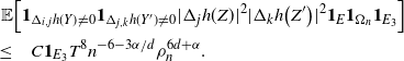 \begin{align}\notag \mathbb{E} & \Big[ \mathbf{1}_{\Delta_{i,j} h(Y) \neq 0} \mathbf{1}_{\Delta_{j,k} h(Y^{\prime}) \neq 0} |\Delta_j h(Z)|^2 |\Delta_k h\big(Z^{\prime}\big)|^2 \mathbf{1}_{E} \mathbf{1}_{\Omega_n} \mathbf{1}_{E_3}\Big] && \\ \leq & \quad C \mathbf{1}_{E_3} T^8 n^{-6 - 3\alpha/d} \rho_n^{6d + \alpha}. &&\end{align}
Finally, for the event
 $E_2$
, assuming that
$E_2$
, assuming that
 $|i - j | \geq |\mathcal{S}| K$
, the other case being identical, we have
$|i - j | \geq |\mathcal{S}| K$
, the other case being identical, we have
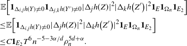 \begin{align}\notag \mathbb{E} & \Big[ \mathbf{1}_{\Delta_{i,j} h(Y) \neq 0} \mathbf{1}_{\Delta_{j,k} h(Y^{\prime}) \neq 0} |\Delta_j h(Z)|^2 |\Delta_k h\big(Z^{\prime}\big)|^2 \mathbf{1}_{E} \mathbf{1}_{\Omega_n} \mathbf{1}_{E_2}\Big]&& \\\notag \leq & \mathbb{E} \Big[ \mathbf{1}_{\Delta_{i,j} h(Y) \neq 0} |\Delta_j h(Z)|^2 |\Delta_k h\big(Z^{\prime}\big)|^2 \mathbf{1}_{E} \mathbf{1}_{\Omega_n} \mathbf{1}_{E_2}\Big]&& \\ \leq & C \mathbf{1}_{E_2} T^6 n^{-5 - 3 \alpha/d} \rho_n^{5d + \alpha}.&&\end{align}
Using (59), (60), (62), and (61) leads to
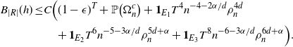 \begin{align}\notag B_{|R|}(h) \leq & C \Big((1 - \epsilon)^T +\mathbb{P}\big(\Omega_n^c\big) + \mathbf{1}_{E_1} T^4 n^{-4 - 2\alpha/d} \rho_n^{4d} \\\notag & \quad +\mathbf{1}_{E_2} T^6 n^{-5 - 3\alpha/d} \rho_n^{5d + \alpha} + \mathbf{1}_{E_3} T^8 n^{-6 -3 \alpha/d} \rho_n^{6d + \alpha}\Big).\end{align}
Then,
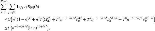 \begin{align}\notag \sum_{i = 0}^{|R| - 1} & \sum_{j, k \notin A} \mathbf{1}_{i \neq j \neq k} B_{|R|} (h) \\\notag \leq & C \Big( n^3 ( 1 - \epsilon)^T + n^3 \mathbb{P}\big(\Omega_n^c\big) + T^6 n^{-3 - 2\alpha/d} \rho_n^{4d} +T^7 n^{-3 - 3\alpha/d} \rho_n^{5d + \alpha} + T^8 n^{-3 - 3\alpha/d} \rho_n^{6d + \alpha}\Big) \\\notag \leq & C \big( n^{-3 - 2 \alpha/d} (\text{ln}\ n)^{10 + 4 \epsilon^{\prime}}\big),\end{align}
where we have chosen
 $K = c \text{ln}\ n$
, for a suitable
$K = c \text{ln}\ n$
, for a suitable
 $c > 0$
, independent of n, using also (58) and the definition of
$c > 0$
, independent of n, using also (58) and the definition of
 $\rho_n$
.
$\rho_n$
.
Funding information
The first author’s research is supported in part by grant no. 524678 from the Simons Foundation. The second author was partially supported by a TRIAD NSF grant (award 1740776) and the FNR grant APOGee at Luxembourg University (R-AGR-3585-10-C).
Competing interests
There were no competing interests to declare which arose during the preparation or publication process for this article.
