2.1. Model equations and assumptions

As illustrated by figure 1(a), we consider dry granular avalanches down erodible slopes of surface inclination $\theta$ close to the critical angle $\theta _c$, and choose axes $(x,z)$ tilted at this angle. We denote by ${\tilde {z}}(x,t)$ and ${\underset{\raise0.3em\hbox{$\smash{\scriptscriptstyle\thicksim}$}}{z}}(x,t)$ the upper and lower boundaries of the flow layer, with $h(x,t) = {\tilde {z}} - {\underset{\raise0.3em\hbox{$\smash{\scriptscriptstyle\thicksim}$}} {z}}$ the corresponding thickness. Local governing equations are then applied to domain ${\underset{\raise0.3em\hbox{$\smash{\scriptscriptstyle\thicksim}$}} {z}} < z < {\tilde {z}}$, subject to the following assumptions. In a drum of width $W$, we consider solid grains of diameter $D$ and density $\rho _S$, and assume dense granular flows for which the solid fraction $c_S$ and bulk density $\rho = c_S \rho _S$ are approximately constant, as supported by experimental observations (MiDi Reference Midi2004). Although the transition from static to flowing typically involves some degree of dilatancy, the resulting changes in volume fraction are assumed small enough to be negligible. Mass conservation therefore reduces to the continuity equation

(2.1)\begin{equation} \frac{\partial u}{\partial x} + \frac{\partial w}{\partial z} = 0, \end{equation}

where $u,w$ are the downslope and normal components of velocity. Secondly, shallow flows are assumed, hence local momentum balance equations parallel and normal to the slope can be written

(2.2)$$\begin{gather} \rho \left( \frac{\partial u}{\partial t} + u\frac{\partial u}{\partial x} + w \frac{\partial u}{\partial z} \right) = \rho g \sin{\theta} + \frac{\partial \tau}{\partial z}, \end{gather}$$

(2.3)$$\begin{gather}\frac{\partial \sigma}{\partial z} ={-}\rho g \cos{\theta}, \end{gather}$$

where $\tau$ and $\sigma$ are respectively the shear and normal granular stresses, and g is the gravitational acceleration. Transverse velocity variations are neglected, and the flows are assumed sufficiently shallow and wide to neglect the influence of sidewall friction. For some granular flows in thin channels, sidewall friction plays a crucial role, as it controls the flow depth attained at steady state over erodible beds (Taberlet et al. Reference Taberlet, Richard, Valance, Losert, Pasini, Jenkins and Delannay2003; Jop et al. Reference Jop, Forterre and Pouliquen2005). Episodic surface avalanches, however, also occur in wide drums, or in discrete element simulations for which sidewalls are replaced by periodic boundary conditions (Han et al. Reference Han, Feng, Zhang, Yang, Zivkovic and Li2021). This indicates that sidewall friction is not a crucial factor for unsteady, discrete avalanching. Even when frictional sidewalls are present, in this work we will assume for simplicity that the ratio of flow depth to drum width remains small enough for sidewall friction to be negligible.

For the shear stress $\tau$ within the flow layer, we assume the linearized $\mu (I)$ rheology (da Cruz et al. Reference da Cruz, Emam, Prochnow, Roux and Chevoir2005)

(2.4)\begin{equation} \tau = \mu(I)\sigma = (\tan\theta_c + \chi \sqrt{\rho/\rho_S} I) \sigma = \tan\theta_c \sigma + \chi D \sqrt{\rho \sigma} \dot{\gamma}, \end{equation}

where $\mu$ is the dimensionless shear to normal stress ratio, $\chi$ a dimensionless rheological coefficient, $\dot {\gamma } = \partial u/\partial z$ the local shear rate and $I = \dot {\gamma }D/\sqrt {\sigma /\rho _S}$ the inertial number. For sustained shear at very slow shear rate, $I \ll 1$, the ratio of shear to normal stress therefore reduces to $\tau /\sigma = \tan \theta _c$, which defines the critical angle of internal friction $\theta _c$. As $\dot {\gamma }$ increases, $\tau$ increases proportionately, with an effective viscosity $\chi D \sqrt {\rho \sigma }$ that varies as the square root of the normal stress $\sigma$. For frictional spheres, experiments (Jop et al. Reference Jop, Forterre and Pouliquen2005; Tapia et al. Reference Tapia, Pouliquen and Guazzelli2019) and discrete element simulations (Azéma & Radjaï Reference Azéma and Radjaï2014) show that the rheological coefficient does not vary greatly with particle properties, and takes the approximate value $\chi \approx 1$. For frictionless particles, simulations with two-dimensional (Bouzid et al. Reference Bouzid, Trulsson, Claudin, Clément and Andreotti2013) and three-dimensional grains (Dumont et al. Reference Dumont, Bonneau, Salez, Raphaël and Damman2023) indicate that, instead of a linear relationship, the rate-dependent component of the shear stress varies roughly with the square root of the shear rate. In this work, we restrict our attention to frictional spheres.

Boundary conditions at the surface and at the base of the flowing layer are formulated as follows. First, we assume zero flux across the free surface $z = {\tilde {z}}$, hence the kinematic boundary condition

(2.5)\begin{equation} \frac{ \partial {\tilde{z}} }{\partial t} + {\tilde{u}} \frac{\partial {\tilde{z}}}{\partial x} = {\tilde{w}}, \end{equation}

where ${\tilde {u}}, {\tilde {w}}$ denote the velocity components along the free surface. At the surface, we also assume no stress, or $\tilde {\tau } = \tilde {\sigma } = 0$. The normal stress then integrates to $\sigma = \rho g_{_{\perp }} y$, where $g_{_{\perp }} = g \cos \theta _c$ and $y = {\tilde {z}} - z$ denotes the depth below free surface. Assuming the rheology (2.4), the shear rate must therefore vanish at the upper free surface. This is at variance with experiments (Capart et al. Reference Capart, Hung and Stark2015) and discrete element simulations (Parez et al. Reference Parez, Aharonov and Toussaint2016), which show instead a finite shear rate at the top. The resulting velocity profiles, however, remain in relatively close agreement.

At the base, we adopt the new boundary conditions proposed recently by Capart (Reference Capart2023) for granular flows over brittle beds. Flow is assumed to take place over an erodible granular substrate, or bed, with which grains can be exchanged. The basal boundary $z = {\underset{\raise0.3em\hbox{$\smash{\scriptscriptstyle\thicksim}$}} {z}}$, representing the interface between the flow and bed, is defined as the uppermost locus where ${\rm \Delta} u = 0$, with ${\rm \Delta} u$ denoting the granular velocity in excess of the bed velocity due to rigid body rotation. For slow drum rotation rates, the bed rotation velocity can be neglected, as it is much smaller than the velocity of avalanching grains. Regardless, the decrease of the excess velocity ${\rm \Delta} u$ to zero at a well-defined finite depth is again an idealization, as actual velocity profiles typically show a more gradual exponential decay or power law decrease to zero at the base.

Subject to this idealization, the basal interface constitutes a sharply defined moving boundary that evolves according to

(2.6)\begin{equation} \frac{\partial {\underset{\raise0.3em\hbox{$\smash{\scriptscriptstyle\thicksim}$}}{z}}}{\partial t} - {\underset{\raise0.3em\hbox{$\smash{\scriptscriptstyle\thicksim}$}}{w}} ={-} e + d. \end{equation}

On the left-hand side, ${\underset{\raise0.3em\hbox{$\smash{\scriptscriptstyle\thicksim}$}} {w}}$ is the velocity at which the basal substrate uplifts (${\underset{\raise0.3em\hbox{$\smash{\scriptscriptstyle\thicksim}$}} {w}} > 0$) or subsides (${\underset{\raise0.3em\hbox{$\smash{\scriptscriptstyle\thicksim}$}} {w}} < 0$) due to drum rotation or sandbox tilting. On the right-hand side, $e \geq 0$ is the rate of erosion or entrainment and $d \geq 0$ the rate of deposition or detrainment, both assumed positive. Whether entrainment ($e>0$) or detrainment ($d>0$) can occur then depends on the shear stress $\underset{\raise0.3em\hbox{$\smash{\scriptscriptstyle\thicksim}$}} {\tau }$ and shear rate $\underset{\raise0.3em\hbox{$\smash{\scriptscriptstyle\thicksim}$}} {\dot {\gamma }}$ attained at the base of the flow layer. For erosion to occur ($e>0$), the basal shear stress must overcome the erosion resistance

(2.7)\begin{equation} \tau_e = \tan\theta_e \sigma, \end{equation}

where $\theta _e > \theta _c$ is an angle of friction describing the bed resistance to erosion: a greater shear stress is needed to unjam bed grains than to keep them flowing at a slow shear rate (Atman et al. Reference Atman, Claudin, Combe and Martins2014; Farain & Bonn Reference Farain and Bonn2023). Note that the angle $\theta _e$, like the failure angle $\theta _f$, does not take a unique value. Instead, it may depend on system history and exhibit random variation from one avalanche to the next. For a single avalanche, however, we will assume $\theta _e$ to be constant. Similar to our assumed gap between $\theta _e$ and $\theta _c$, Dumont et al. (Reference Dumont, Soulard, Salez, Raphaël and Damman2020) conducted discrete element simulations of heap and inclined plane flows of frictional spheres in which they found a significant gap between erosion and sedimentation angles.

Accordingly, when $e>0$, the shear stress at the base of the flowing layer must satisfy

(2.8)\begin{equation} \underset{\raise0.3em\hbox{$\smash{\scriptscriptstyle\thicksim}$}}{\tau} = \tan\theta_e \underset{\raise0.3em\hbox{$\smash{\scriptscriptstyle\thicksim}$}}{\sigma} = \tan\theta_c \underset{\raise0.3em\hbox{$\smash{\scriptscriptstyle\thicksim}$}}{\sigma} + \chi D \sqrt{ \rho \underset{\raise0.3em\hbox{$\smash{\scriptscriptstyle\thicksim}$}}{\sigma}}\underset{\raise0.3em\hbox{$\smash{\scriptscriptstyle\thicksim}$}}{\dot{\gamma}}, \end{equation}

where $\underset{\raise0.3em\hbox{$\smash{\scriptscriptstyle\thicksim}$}} {\sigma } = \rho g_{_{\perp }} h$ is the normal stress at the base. For entrainment to occur, the requisite shear stress must be provided by rapidly sheared near-bed grains. Thus the basal shear rate has to reach the maximal value

(2.9)\begin{equation} \underset{\raise0.3em\hbox{$\smash{\scriptscriptstyle\thicksim}$}}{\dot{\gamma}}_{max} = \frac{\tan\theta_e - \tan\theta_c}{\chi D} \sqrt{ g_{_{{\perp}}} h }, \end{equation}

proportional to the difference between the two friction coefficients $\tan \theta _e$ and $\tan \theta _c$. For detrainment to occur ($d>0$), on the other hand, we assume that the basal shear rate must decrease to zero. The entrainment and detrainment rates $e,d$ are therefore governed by the following complementary inequalities

(2.10a–c)$$\begin{gather} e \geq 0,\quad \underset{\raise0.3em\hbox{$\smash{\scriptscriptstyle\thicksim}$}}{\dot{\gamma}} \leq \underset{\raise0.3em\hbox{$\smash{\scriptscriptstyle\thicksim}$}}{\dot{\gamma}}_{max},\quad (\underset{\raise0.3em\hbox{$\smash{\scriptscriptstyle\thicksim}$}}{\dot{\gamma}} - \underset{\raise0.3em\hbox{$\smash{\scriptscriptstyle\thicksim}$}}{\dot{\gamma}}_{max})e = 0, \end{gather}$$

(2.11a–c)$$\begin{gather}d \geq 0,\quad \underset{\raise0.3em\hbox{$\smash{\scriptscriptstyle\thicksim}$}}{\dot{\gamma}} \geq 0,\quad \underset{\raise0.3em\hbox{$\smash{\scriptscriptstyle\thicksim}$}}{\dot{\gamma}} d = 0. \end{gather}$$

By eroding or depositing grains as needed, the flow layer thus maintains its basal shear rate within a finite range, bracketed by the following lower and upper bounds:

(2.12)\begin{equation} 0 \leq \underset{\raise0.3em\hbox{$\smash{\scriptscriptstyle\thicksim}$}}{\dot{\gamma}} \leq \underset{\raise0.3em\hbox{$\smash{\scriptscriptstyle\thicksim}$}}{\dot{\gamma}}_{max}. \end{equation}

Conversely, these bounds must be attained for the flow to erode or deposit grains. If the bounds are not attained, $0 < \underset{\raise0.3em\hbox{$\smash{\scriptscriptstyle\thicksim}$}} {\dot {\gamma }} < \underset{\raise0.3em\hbox{$\smash{\scriptscriptstyle\thicksim}$}} {\dot {\gamma }}_{max}$, we assume that the flow can neither entrain or detrain, and call this situation bypass. These three possible basal behaviours – entrainment, bypass and detrainment – are illustrated in figure 2. As the flow evolves over time, the conditions (2.10a–c) and (2.10a–c) allow the flow to transition continuously between these three behaviours.

Figure 2. Three possible solution behaviours dependent on the basal shear rate: (a) entrainment, possible only when the shear rate is maximal (dashed blue line); (b) bypass, when the basal shear rate is intermediate; (c) detrainment, possible only when the basal shear rate is zero (dashed magenta line). Arrows up or down denote basal interface motions, and a cross the absence of such motion.

2.2. Reduced equations

Integrated over depth, the local continuity equation (2.1) yields an evolution equation for the surface profile ${\tilde {z}}(x,t)$

(2.13)\begin{equation} \frac{\partial {\tilde{z}}}{\partial t} + \frac{ \partial q }{\partial x} = {\underset{\raise0.3em\hbox{$\smash{\scriptscriptstyle\thicksim}$}}{w}}, \end{equation}

where $q = \int u\,{\rm d} z$ is the discharge per unit width. Upon invoking (2.6), we can then deduce

(2.14)\begin{equation} \frac{\partial h}{\partial t} + \frac{\partial q}{\partial x} = e - d. \end{equation}

The erosion and deposition rates $e,d$ thus affect the evolution of the flow thickness $h$, but do not directly affect the evolution of the free surface elevation ${\tilde {z}}$. For application to rotating drums, the basal velocity ${\underset{\raise0.3em\hbox{$\smash{\scriptscriptstyle\thicksim}$}} {w}}$ induced by drum rotation can be expressed

(2.15)\begin{equation} {\underset{\raise0.3em\hbox{$\smash{\scriptscriptstyle\thicksim}$}}{w}} ={-}\varOmega x, \end{equation}

where $\varOmega$ is the drum rotation rate, and with the origin $x=0$ placed at mid-slope. When the drum is slowly rotated, episodic avalanches occur, during which the surface inclination drops rapidly, alternating with periods of no flow and gradual re-steepening. Both during and between slope relaxation events, experiments indicate that the surface profile ${\tilde {z}}(x,t)$ can be well approximated by a straight line of time-varying inclination

(2.16)\begin{equation} {\tilde{z}}(x,t) ={-} (\theta(t)-\theta_c)x. \end{equation}

Substitution of (2.15) and (2.16) into (2.13) produces

(2.17)\begin{equation} \frac{\partial q}{\partial x} = \left(\frac{{\rm d}\theta}{{\rm d} t} - \varOmega\right) x. \end{equation}

Integration subject to boundary conditions $q=0$ at $x = \pm L/2$ then yields

(2.18)\begin{equation} q(x,t) = \frac{(L/2)^2 - x^2}{2}\left(\varOmega-\frac{{\rm d}\theta}{{\rm d} t}\right). \end{equation}

By assuming that the free surface remains perfectly straight, with a time-dependent but uniform inclination, we therefore constrain the flow discharge to evolve synchronously everywhere along the slope. Thus we neglect the local surface irregularities and propagation dynamics that can be observed in both experiments (Balmforth & McElwaine Reference Balmforth and McElwaine2018) and discrete element simulations (Han et al. Reference Han, Feng, Zhang, Yang, Zivkovic and Li2021). In what follows, we will assume very slow steepening rates ($\varOmega \ll -{\rm d}\theta /{\rm d} t$) and focus on the comparatively fast slope relaxation events. Applying (2.18) at mid-slope then yields for the inclination $\theta (t)$ the ordinary differential equation (Courrech du Pont et al. Reference Courrech du Pont, Fischer, Gondret, Perrin and Rabaud2005)

(2.19)\begin{equation} \frac{{\rm d}\theta}{{\rm d} t} ={-} \frac{8}{L^2} q(0,t), \end{equation}

involving only the discharge $q(0,t)$ at mid-slope ($x=0$), where ${\tilde {z}}(0,t) = 0$. At mid-slope, moreover, $\partial q/\partial x = 0$ and the flow is approximately uniform, so that convective acceleration terms can be safely neglected. The local momentum balance equation (2.2) can therefore be approximated there by

(2.20)\begin{equation} \rho \frac{\partial u}{\partial t} = \rho g \sin{\theta} + \frac{\partial \tau}{\partial z}. \end{equation}

Substitution of the rheology (2.4) then yields

(2.21)\begin{equation} \frac{\partial u}{\partial t} = g_{_{{\perp}}} (\tan\theta-\tan\theta_c) + g_{_{{\perp}}}^{1/2} \chi D \frac{\partial}{\partial y}\left( y^{1/2} \frac{\partial u}{\partial y}\right), \end{equation}

where it is convenient to use the depth coordinate $y = {\tilde {z}}-z$ instead of $z$. Upon defining the excess slope $S(t)$ by

(2.22)\begin{equation} S(t) = \tan\theta(t) - \tan\theta_c, \end{equation}

we can approximate ${\rm d}\theta /{\rm d} t = \cos ^2\theta _c \,{\rm d} S/{\rm d} t$. We can therefore describe the relaxation of slopes of finite length using two coupled equations. The first is an ordinary differential equation for the excess slope

(2.23)\begin{equation} \cos^2\theta_c \frac{{\rm d} S}{{\rm d} t} ={-} \frac{8}{L^2} \int_0^h u {{\rm d}y}, \end{equation}

featuring on the right-hand side the integral of the velocity profile at mid-slope, $u(y,t)$. The second is a partial differential equation for this velocity profile

(2.24)\begin{equation} \frac{\partial u}{\partial t} = g_{_{{\perp}}} S(t) + g_{_{{\perp}}}^{1/2} \chi D \frac{\partial}{\partial y}\left(y^{1/2} \frac{\partial u}{\partial y}\right)\quad (0 < y < h), \end{equation}

where the excess slope $S(t)$ intervenes as a time-dependent forcing term. The velocity profile is subject to three boundary conditions, one at the free surface and two at the base

(2.25)$$\begin{gather} \frac{\partial u}{\partial y} = 0\quad (y=0), \end{gather}$$

(2.26)$$\begin{gather}u = 0,\quad 0\leq{-}\frac{\partial u}{\partial y} \leq \frac{\tan\theta_e-\tan\theta_c}{\chi D}\sqrt{g_{_{{\perp}}} h}\quad (y=h). \end{gather}$$

Two boundary conditions are needed at the base because the time-evolving flow thickness $h(t)$ is also unknown. For the initial conditions, finally, we assume that the granular slope starts from rest, at failure time $t_f$ and failure angle $\theta _f$, with a flow layer of zero initial thickness $h_f = 0$.

Assuming slow rotation rates, note that the equations derived here apply to arbitrary drum fill level $l$, the influence of which we capture via the slope length $L$. Following Gray (Reference Gray2001), we define the fill level $l$ as the offset distance of the flat free surface away from the drum centre. The slope length is then $L = 2\sqrt { R^2 - l^2}$, and reduces to $L = 2R$ when the drum is half-filled ($l = 0$). Provided that the correct slope length $L$ is used, all our results continue to hold when $l \neq 0$, motivating our choice of $L$ instead of $R$ as our defining length. In § 5, we will need this flexibility to apply the theory to the discrete element simulations of Kasper et al. (Reference Kasper, Magnanimo, de Jong, Beek and Jarray2021), for which the drum was not half-filled. Prior to solving the equations, it is useful to first cast them in dimensionless form. For this purpose, a scaling analysis is conducted in the next section.

2.3. Scaling analysis

To make the equations dimensionless, let us adopt the slope length $L$ as length scale, and $S_e = \tan \theta _e-\tan \theta _c$ as slope scale. We then seek time, velocity and depth scales $T$, $U$ and $H$ that balance the different terms of the reduced equations. From (2.23), we deduce

(2.27)\begin{equation} \cos^2\theta_c \frac{S_e}{T} = \frac{HU}{L^2}. \end{equation}

From (2.24), on the other hand, we get

(2.28)\begin{equation} \frac{U}{T} = g_{_{{\perp}}} S_e = \frac{g_{_{{\perp}}}^{1/2}\chi D U}{H^{3/2}}. \end{equation}

For the depth scale, we obtain

(2.29)\begin{equation} H = (\chi D L\cos\theta_c)^{1/2}. \end{equation}

The depth scale $H$ is therefore proportional to the geometric mean of the grain diameter $D$ and slope length $L$, a surprisingly simple result that does not seem to have been reported previously. For the time scale, we deduce

(2.30)\begin{equation} T = \frac{(L\cos\theta_c)^{3/4}}{g_{_{{\perp}}}^{1/2}(\chi D)^{1/4}}, \end{equation}

proportional to the slope length $L$ raised to the power $3/4$, and inversely proportional to the grain diameter $D$ to the power $1/4$. For the velocity scale, finally, we get

(2.31)\begin{equation} U = g_{_{{\perp}}}^{1/2} \frac{(L\cos\theta_c)^{3/4}}{(\chi D)^{1/4}}S_e, \end{equation}

proportional to the slope scale $S_e$. We use these scales to define the dimensionless variables

(2.32a–f)\begin{equation} y^* = \frac{y}{H},\quad h^* = \frac{h}{H},\quad t^*=\frac{t-t_f}{T},\quad S^* = \frac{S}{S_e},\quad u^* = \frac{u}{U},\quad \dot{\gamma}^* = \frac{\dot{\gamma}}{U/H}. \end{equation}

The governing equations then become, in dimensionless form,

(2.33)$$\begin{gather} \frac{{\rm d} S^*}{{\rm d} t^*} ={-}8 \int_0^{h^*} u^* \,{{\rm d}y}^*, \end{gather}$$

(2.34)$$\begin{gather}\frac{\partial u^*}{\partial t^*} = S^* + \frac{\partial}{\partial y^*}\left( y^{*1/2} \frac{\partial u^*}{\partial y^*} \right), \end{gather}$$

with boundary conditions

(2.35)$$\begin{gather} \frac{\partial u^*}{\partial y^*}=0\quad (y^* = 0), \end{gather}$$

(2.36)$$\begin{gather}u^*=0,\quad 0 \leq{-}\frac{\partial u^*}{\partial y^*} \leq h^{*1/2}\quad (y^* = h^*), \end{gather}$$

and initial conditions

(2.37)\begin{equation} h^* = 0,\quad S^* = S^*_f = \frac{\tan\theta_f-\tan\theta_c}{\tan\theta_e-\tan\theta_c} \approx \frac{\theta_f-\theta_c}{\theta_e-\theta_c}\quad (t^*=t^*_f = 0). \end{equation}

The number $S^*_f$, the only dimensionless number that remains, represents the over-steepening of the slope at failure. It is defined as the ratio of excess slope at failure to excess resistance to erosion. Remarkably, the failure and erosion resistance inclinations $\theta _f$ and $\theta _e$ affect the dimensionless dynamics of discrete avalanches only jointly, via this number $S^*_f$. Analogous to the brittleness index introduced by Bishop (Reference Bishop1971), it provides a dimensionless measure of the brittleness, or degree of metastability of the slope.

Mathematically, we obtain a rather unusual system coupling one integro-differential equation for the slope $S^*(t^*)$ (2.33), with one partial differential equation for the velocity profile $u^*(y^*,t^*)$ (2.34). To solve this system, we need to examine in sequence three distinct stages, characterized respectively by entrainment, bypass and detrainment. In the next section, analytical techniques will be used to derive solutions for each stage.

3.1. Entrainment stage

Upon failure, the avalanching layer must first entrain grains from the underlying substrate. For erosion to occur, the basal shear rate must attain its upper limit

(3.1)\begin{equation} {-}\frac{\partial u^*}{\partial y^*}(y^*=h^*) = \underset{\raise0.3em\hbox{$\smash{\scriptscriptstyle\thicksim}$}}{\dot{\gamma}}^*_{max} = h^{*1/2}. \end{equation}

By analogy with the constant slope case treated in Capart (Reference Capart2023), we seek an exact similarity solution whereby the flowing layer simultaneously thickens and accelerates, while maintaining a velocity profile of Bagnold shape. The time-evolving velocity profile satisfying the boundary conditions at the surface and at the base is then

(3.2)\begin{equation} u^*(y^*,t^*) =\begin{cases} \frac{2}{3}(h^*(t^*)^{3/2}-y^{*3/2}), & 0\leq y^* \leq h^*(t^*),\\ 0, & h^*(t^*)\leq y^*, \end{cases} \end{equation}

where $h^*(t^*)$ is the flow thickness evolution, yet to be determined. Substituting this ansatz into the mass and momentum balance equations (2.33) and (2.34) yields

(3.3)$$\begin{gather} \frac{{\rm d} S^*}{{\rm d} t^*} ={-}\frac{16}{5}h^{*5/2}, \end{gather}$$

(3.4)$$\begin{gather}h^{*1/2}\frac{{\rm d} h^*}{{\rm d} t^*} = S^* - 1, \end{gather}$$

which form a pair of nonlinear ordinary differential equations (ODEs) for the coupled time evolution of the avalanche slope $S^*(t^*)$ and thickness $h^*(t^*)$. Note that the Bagnold velocity profile does not represent an extra assumption or approximation on our part, nor is it restricted to flows over a non-erodible base. For the entrainment stage, the time-evolving Bagnold profile (3.2) is the exact solution to the assumed governing equations, boundary and initial conditions, provided that the two ODEs (3.3) and (3.4) are satisfied. This was derived step by step in Capart (Reference Capart2023), and can be checked by direct substitution into (2.33) to (2.37). During bypass and detrainment, the Bagnold shape no longer applies and the velocity profile deforms into a sigmoidal shape.

To solve the equations, the time variable can be eliminated from (3.4) by using the chain rule together with (3.3), yielding the separable ODE

(3.5)\begin{equation} h^{*1/2}\frac{{\rm d} h^*}{{\rm d} S^*}\frac{{\rm d} S^*}{{\rm d} t^*} ={-}\frac{16}{5}h^{*3}\frac{{\rm d} h^*}{{\rm d} S^*} = S^*-1. \end{equation}

This can be integrated with initial conditions $S^* = S^*_f$ and $h^*=0$ at time $t^*_f = 0$, to get

(3.6)\begin{equation} h^*(S^*) = \left(\tfrac{5}{8}\right)^{1/4}((S^*_f-1)^2-(S^*-1)^2)^{1/4}. \end{equation}

The flow layer thickness increases until $S^* = S^*_e = 1$, where it saturates at the extremal value

(3.7)\begin{equation} h^*_e = \left(\tfrac{5}{8}\right)^{1/4} (S^*_f-1)^{1/2}, \end{equation}

retained during the ensuing bypass stage. By integrating the profile (3.2) over depth, we can also calculate the discharge evolution

(3.8)\begin{equation} q^*(S^*) = \tfrac{2}{5}\left(\tfrac{5}{8}\right)^{5/8}((S^*_f-1)^2-(S^*-1)^2)^{5/8}. \end{equation}

The resulting orbits are shown in figure 3(a), for five different values of $S^*_f$. The discharge peaks at the end of the entrainment stage ($S^* = S^*_e =1$), reaching the maximum value

(3.9)\begin{equation} q^*_e = \tfrac{2}{5}\left(\tfrac{5}{8}\right)^{5/8} (S^*_f-1)^{5/4}. \end{equation}

Upon defining $S^{\prime } = S^*-1$, $\hat {S}^{\prime } = S^{\prime }/S_f^{\prime }$ and $\hat {q}=q^*/q^*_e$, the slope-discharge relationship can also be written

(3.10)\begin{equation} \hat{S}^{\prime 2} + (\hat{q}^{4/5})^2 = 1. \end{equation}

In the $(\hat {S}^{\prime },\hat {q}^{4/5})$ plane, the orbits trace a unit circle centred at the origin. In the $(S^*,q^*)$ plane, as illustrated in figure 3(a), the orbits become slightly distorted. Different failure slopes $S^*_f$ yield geometrically similar orbits (scaled copies of each other) with similarity centre $(S^*_e,0)=(1,0)$. Starting from rest, no self-accelerating erosion can occur if $S^*_f\leq 1$. Beyond this threshold, the greater the oversteepening at failure, the greater the maximum discharge attained by the resulting avalanche.

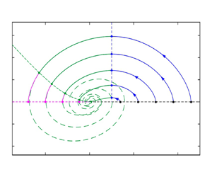
Figure 3. Solution curves for slopes of varying brittleness, during successive evolution stages: (a,b) solutions for the entrainment stage (blue lines) and their continuation beyond their domain of validity (long blue dashes); (c,d) solutions for the bypass stage (green lines) and their continuation beyond their domain of validity (long green dashes); (e,f) solutions for the detrainment stage (magenta lines). Short dashes: domain boundaries.

To obtain the time evolution, the solution (3.6) can be substituted back into (3.3) to get

(3.11)\begin{equation} \frac{{\rm d} S^*}{{\rm d} t^*} ={-}2\left(\frac{8}{5}\right)^{3/8}((S^*_f-1)^2-(S^*-1)^2)^{5/8}. \end{equation}

Defining $\hat {t} = 2(\frac {8}{5})^{3/8} S^{\prime 1/4}_f t^*$, this ODE can be normalized and separated into

(3.12)\begin{equation} \frac{{\rm d}\hat{S}^{\prime}}{(1-\hat{S}^{\prime 2})^{5/8}} ={-} {\rm d}\hat{t}. \end{equation}

Integration subject to initial condition $\hat {S}^{\prime }(0)=1$ then yields the implicit solution

(3.13)\begin{equation} G_{5/4}(\hat{S}^{\prime}) - G_{5/4}(1)={-}\hat{t}. \end{equation}

Here, we have introduced the generalized arcsine function

(3.14)\begin{equation} G_\varphi(x) = \int_0^x\frac{{\rm d}\xi}{(1-\xi^2)^{\varphi/2}} = x {}_2F_1\left(\frac{1}{2},\frac{\varphi}{2};\frac{3}{2};x^2\right), \end{equation}

where $_2F_1(a,b;c,x)$ is the hypergeometric function. Defined over interval $-1\leq x \leq 1$, $G_\varphi (x)$ is an odd function that resembles an arcsine and in fact reduces to $G_1(x) = \sin ^{-1}(x)$ when $\varphi = 1$. The normalized time at which $\hat {S}^{\prime }=0$, erosion ends and the discharge peaks is then given by

(3.15)\begin{equation} \hat{t}_e = G_{5/4}(1) = \int_0^1\frac{{\rm d}\kern 0.06em x}{(1-x^2)^{5/8}} = \frac{\sqrt{\rm \pi}\varGamma\left(\dfrac{3}{8}\right)}{2\varGamma\left(\dfrac{7}{8}\right)} \approx 1.9279, \end{equation}

where $\varGamma ({\cdot })$ is the gamma function. In terms of dimensionless variables (2.36), this result can also be written

(3.16)\begin{equation} t^*_e = \tfrac{1}{2}\left(\tfrac{5}{8}\right)^{3/8}\hat{t}_e (S^*_f-1)^{{-}1/4} = \tfrac{1}{4}\left(\tfrac{5}{2}\right)^{3/10}\hat{t}_e q^{*-1/5}_e. \end{equation}

Thus the greater the oversteepening at failure, the greater the peak discharge, and the shorter the time needed to attain this peak. This is illustrated in figure 3(b), which shows the dimensionless discharge hydrographs $q^*(t^*)$ associated with the orbits of figure 3(a). Note that the results of this section are valid only for the entrainment stage, over time interval $t^*_f = 0 \leq t^* \leq t^*_e$. The corresponding curve segments are shown as solid lines on figure 3(a,b). To show what the formulas produce beyond this range of validity, however, the corresponding curves are also shown as dashed lines. The correct curves for $t^*>t^*_e$ are derived in the next sections.

3.2. Bypass stage

At time $t^* = t^*_e$, the flow layer starts to decelerate. Detrainment cannot yet occur, however, because the basal shear rate $\underset{\raise0.3em\hbox{$\smash{\scriptscriptstyle\thicksim}$}} {\dot {\gamma }}^*$ at this time still has the maximal value

(3.17)\begin{equation} \underset{\raise0.3em\hbox{$\smash{\scriptscriptstyle\thicksim}$}}{\dot{\gamma}}^*_{max} = h^{*1/2}_e. \end{equation}

Starting from this finite value, the basal shear rate must drop back to zero before deposition can occur. Over some time $t^*_e\leq t^* \leq t^*_d$, the flowing layer will therefore undergo bypass, during which it will retain the constant thickness $h^* = h^*_e$ given by (3.7). During the bypass stage, the Bagnold shape (3.2) no longer holds, hence the evolving shape of the velocity profile must be derived anew. The equations to be solved can be written

(3.18)$$\begin{gather} \frac{{\rm d} S^*}{{\rm d} t^*} ={-}8h^*_e \int_0^1 u^* \,{\rm d}\eta, \end{gather}$$

(3.19)$$\begin{gather}\frac{\partial u^*}{\partial t^*} = S^* + \frac{1}{h^{* 3/2}_e} \frac{\partial}{\partial \eta}\left(\eta^{1/2} \frac{\partial u^*}{\partial \eta}\right), \end{gather}$$

where $\eta = y/h = y^*/h^*$ is a normalized depth coordinate, and where the evolving velocity profile $u^*(\eta,t^*)$ must satisfy the homogeneous boundary conditions

(3.20a,b)\begin{equation} \frac{\partial u^*}{\partial \eta}(0,t^*) = 0,\quad u^*(1,t^*) = 0. \end{equation}

Given at time $t^*=t^*_e$, the initial conditions for the slope and velocity profile are

(3.21a,b)\begin{equation} S^*(t^*_e) = 1,\quad u^*(\eta,t^*_e) = \tfrac{2}{3}h^{*3/2}_e(1-\eta^{3/2}), \end{equation}

as obtained in the previous section. Whereas for the entrainment stage a nonlinear moving boundary problem had to be solved, here the flow thickness remains constant. The equations therefore become linear and homogeneous: they are linear in the two unknowns $S^*$ and $u^*$, and admit the solution pair $u^*=0$, $S^*=0$. Moreover, their behaviour depends on the single dimensionless number $h^*_e = (\frac {5}{8})^{1/4} (S^*_f-1)^{1/2}$, which itself depends only on the oversteepening at failure, $S^*_f$.

Generalizing an approach applied earlier by Parez et al. (Reference Parez, Aharonov and Toussaint2016) and Capart (Reference Capart2023) to the constant slope case, we seek series solutions for $S^*(t)$ and $u^*(\eta,t^*)$ of the form

(3.22)$$\begin{gather} S^*(t^*) = \sum_{n=1}^{N}C_n \exp(-\lambda_n (t^*-t^*_e)), \end{gather}$$

(3.23)$$\begin{gather}u^*(\eta,t^*) = \sum_{n=1}^{N} C_n\, f_n(\eta)\exp(-\lambda_n (t^*-t^*_e)), \end{gather}$$

where the roots $\lambda _n$ and coefficients $C_n$ can be real or complex, and the infinite series is truncated to a finite number of terms $N=8$ (in practice, $N=3$ is sufficient for accuracy to at least three significant figures). The eigenfunctions $f_n(\eta )$ that satisfy the partial differential equation (3.19) and boundary conditions (3.20a,b) are obtained as

(3.24)\begin{equation} f_n(\eta) = \frac{\eta^{1/4}{\rm J}_{{-}1/3}(\kappa_n \eta^{3/4}) - {\rm J}_{{-}1/3}(\kappa_n)}{\lambda_n {\rm J}_{{-}1/3}(\kappa_n)}, \end{equation}

where $\kappa _n = \tfrac {4}{3}\lambda _n^{1/2}h^{*3/4}_e$, and ${\rm J}_\nu (z)$ is the Bessel function of the first kind of order $\nu$. To satisfy (3.18), the roots $\lambda _n$ must satisfy the transcendental equation

(3.25)\begin{equation} K(\lambda) = (\lambda^2 + 8 h^*_e) {\rm J}_{{-}1/3}(\kappa) - 8 h^{*1/4}_e \frac{{\rm J}_{2/3}(\kappa)}{\lambda^{1/2}} = 0, \end{equation}

in which $\kappa = \frac {4}{3}\lambda ^{1/2}h^{*3/4}_e$. Note that $K(\lambda )$ is a complex-valued function of a complex variable, hence we must find roots $\lambda$ in the complex plane that zero both its real and imaginary parts. The condition (3.25) yields infinitely many discrete roots $\lambda _n$, $n = 1,\ldots,\infty$, indexed by taking the real part of $\lambda _n$ in ascending order. For selected values of the slope brittleness $S^*_f$, the first three calculated roots $\lambda _n$, $n = 1,\ldots,3$ are listed in table 1. The real parts of all roots are positive, yielding, as expected, solutions that decay over time. All roots starting from $n=3$ are real and distinct. For $n>3$, the values $\kappa _n$ can be approximated by the zeros of ${\rm J}_{-1/3}(\kappa )$, the roots obtained earlier for the constant slope case (Capart Reference Capart2023). For the first three roots, however, the variable slope condition (3.25) must be used.

Table 1. First calculated roots $\lambda _n$ and coefficients $C_n$ of the bypass series solution.

The character of the first two roots depends on the value of $S_f^*$ relative to the value $S^*_{f,{crit}} \approx 1.4976$ at which critical damping occurs. For $1 < S^*_f < S^*_{f,{crit}}$, the first two roots are real and distinct, $0 < \lambda _1 < \lambda _2$. For $S^*_f > S^*_{f,{crit}}$, by contrast, the first two roots are complex conjugate, $\lambda _{1,2} = \alpha \pm i \beta$. The value $S^*_f = S^*_{f,{crit}}$ therefore marks a transition from overdamping to underdamping. For avalanching flows started from $S^*_f < S^*_{f,{crit}}$, the flowing layer decelerates asymptotically to zero. Likewise, the basal shear rate $\underset{\raise0.3em\hbox{$\smash{\scriptscriptstyle\thicksim}$}} {\dot {\gamma }}^*$ decreases asymptotically to zero, without ever reaching zero and triggering detrainment. For avalanching flows started from $S^*_f >S^*_{f,{crit}}$, on the other hand, the flowing layer decelerates more strongly, and reaches zero basal shear rate in finite time. This finite time $t^* = t^*_d$ at which detrainment starts is again dependent on $h^*_e$, or equivalently on $S^*_f$.

The coefficients $C_n$, finally, must be chosen to satisfy the initial conditions (3.20a,b). In table 1, we provide calculated values for the first three coefficients, for selected values of $S^*_f$. As needed to satisfy the initial condition $S^*(t^*_e) = 1$, it can be checked that the coefficients $C_n$ sum to 1 in each case. Once the coefficients $C_n$ are known, the time-evolving discharge can be obtained from

(3.26)\begin{equation} q^*(t^*) = h^*_e\int_0^1 u^*(\eta)\,{\rm d}\eta = \sum_{n=1}^{N} \frac{\lambda_n C_n}{8} \exp(-\lambda_n (t^*-t^*_e)). \end{equation}

Likewise the time-evolving basal shear rate can be calculated from

(3.27)\begin{equation} \underset{\raise0.3em\hbox{$\smash{\scriptscriptstyle\thicksim}$}}{\dot{\gamma}}^*(t^*) = \sum_{n=1}^{N} C_n^{\prime} \exp(-\lambda_n (t^*-t^*_e)), \end{equation}

where

(3.28)\begin{equation} C_n^{\prime} ={-}\frac{C_n}{h^*_e}\frac{{\rm d} f_n}{{\rm d}\eta}(1) =\left( \frac{{\rm J}_{2/3}(\kappa_n)-{\rm J}_{{-}4/3}(\kappa_n)}{2\lambda_n^{1/2}h^{*1/4}_e {\rm J}_{{-}1/3}(\kappa_n)} - \frac{1}{4\lambda_nh^*_e} \right)C_n. \end{equation}

If $S_f^*>S_{f,{crit}}$, this basal shear rate drops to zero at the finite time $t^*_d$. To find this time, we approximate the series (3.27) at $t^*_d$ by its first two terms, with complex conjugate coefficients $C^{\prime }_{1,2} = A\pm i B$, such that

(3.29)\begin{equation} \underset{\raise0.3em\hbox{$\smash{\scriptscriptstyle\thicksim}$}}{\dot{\gamma}}^*(t^*_d) \approx (2A \cos(\beta(t^*_d-t^*_e)) + 2B \sin(\beta(t^*_d-t^*_e))) \exp(-\alpha(t^*_d-t^*_e)). \end{equation}

The time $t^*_d$ at which $\underset{\raise0.3em\hbox{$\smash{\scriptscriptstyle\thicksim}$}} {\dot {\gamma }}^*(t^*_d)=0$ is therefore obtained as

(3.30)\begin{equation} t^*_d \approx t^*_e + \frac{1}{\beta}\tan^{{-}1}({-}A/B). \end{equation}

By sampling (3.22) and (3.23) at time $t^*_d$, we can also determine the slope $S^*_d = S^*(t^*_d)<0$ and velocity profile $u^*_d(\eta ) = u^*(\eta,t^*_d)$ attained when detrainment starts.

For the values of $S^*_f$ listed in table 1, the resulting orbits $(S^*(t^*),q^*(t^*))$ are plotted in figure 3(c) (green curves). For $S^*_f=1.4$, the solution is overdamped, and reaches the origin $(0,0)$ without ever leaving the upper half-plane. The other orbits are underdamped, and would eventually spiral inwards to the origin if the basal shear rate did not first drop to zero. The locus $\underset{\raise0.3em\hbox{$\smash{\scriptscriptstyle\thicksim}$}} {\dot {\gamma }}^*=0$ across which this occurs (short green dashes) is located in the upper left quadrant of the $(S^*,q^*)$ plane. The flow therefore reaches zero basal shear rate before the discharge $q^*$ becomes negative. The corresponding discharge hydrographs $q^*(t^*)$ are plotted in figure 3(d). Valid solutions for the bypass stage (continuous green lines) are restricted to the time interval $t^*_e \leq t^* \leq t^*_d$, during which the basal shear rate remains positive. The underdamped curves are also plotted beyond this range (dashed green lines), but only to show their oscillatory behaviour. The correct curves for $t^*>t^*_d$ are derived in the next section.

3.3. Detrainment stage

During the detrainment stage, the flow simultaneously thins and decelerates. We are thus back to a moving boundary problem, this time with a given initial velocity profile at dimensionless time $t^* = t^*_d$. For this stage an exact analytical solution is out of reach, but an approximate semi-analytical solution can be obtained. For this purpose, we let both the flow layer thickness $h^*$ and mean velocity $\bar {u}^{*} = q^*/h^*$ evolve over time, but assume that the velocity profile maintains the self-similar shape

(3.31)\begin{equation} \frac{u^*(\eta,t^*)}{\bar{u}^{*}(t^*)} = \frac{u^*(\eta,t^*_d)}{\bar{u}^{*}(t^*_d)}, \end{equation}

inherited from the bypass solution at time $t^* = t^*_d$. Self-similarity does not hold exactly, but is supported by numerical solutions of stopping transients (Capart et al. Reference Capart, Hung and Stark2015; Barker & Gray Reference Barker and Gray2017). Subject to this assumption, only three variables $S^*(t^*)$, $h^*(t^*)$ and $\bar {u}^*(t^*)$ suffice to describe the system. Like before, the slope must satisfy

(3.32)\begin{equation} \frac{{\rm d} S^*}{{\rm d} t^*} ={-}8 h^* \bar{u}^{*}. \end{equation}

Subject to the basal boundary condition $\underset{\raise0.3em\hbox{$\smash{\scriptscriptstyle\thicksim}$}} {\dot {\gamma }}^* = 0$, appropriate for detrainment, we integrate (2.34) over the flow depth to obtain the momentum balance equation

(3.33)\begin{equation} \frac{{\rm d}}{{\rm d} t^*}(h^*\bar{u}^{*}) = h^* S^*. \end{equation}

Finally, we follow Capart et al. (Reference Capart, Hung and Stark2015) and integrate over depth $u^*$ times (2.34) to obtain a balance equation for the kinetic energy of the flow layer

(3.34)\begin{equation} \frac{{\rm d}}{{\rm d} t^*}\left(\frac{1}{2}\varphi h^*\bar{u}^{*2}\right) = h^*\bar{u}^{*}S^* - \psi\frac{\bar{u}^{*2}}{h^{*1/2}}, \end{equation}

where $\varphi$ (Boussinesq coefficient) and $\psi$ are the two shape factors defined by

(3.35a,b)\begin{equation} \varphi = \frac{1}{h \bar{u}^{2}}\int_0^h u^2 \,{{\rm d}y},\quad \psi = \frac{h^{1/2}}{\bar{u}^{2}} \int_0^h y^{1/2}\dot{\gamma}^2 \,{{\rm d}y}. \end{equation}

Under the similarity assumption (3.31), both $\varphi$ and $\psi$ remain constant during detrainment. Using the product rule and taking quasilinear combinations of (3.33) and (3.34), we deduce the following evolution equations for the flow depth and mean velocity:

(3.36)$$\begin{gather} \frac{1}{2}\varphi\bar{u}^{*}\frac{{\rm d} h^*}{{\rm d} t^*}= (\varphi-1)h^*S^* +\psi \frac{\bar{u}^{*}}{h^{*1/2}}, \end{gather}$$

(3.37)$$\begin{gather}\frac{1}{2}\varphi h\frac{{\rm d}\bar{u}^{*}}{{\rm d} t^*}=(1-\tfrac{\varphi}{2})h^*S^* - \psi \frac{\bar{u}^{*}}{h^{*1/2}}. \end{gather}$$

Together, the three equations (3.32), (3.36) and (3.37) form a closed system of three coupled nonlinear ODEs for $S^*(t^*)$, $h^*(t^*)$ and $\bar {u}^*(t^*)$. Unless $\psi = 0$ is assumed, no closed form solution could be found. The equations can, however, be integrated numerically, starting from the known initial conditions

(3.38a–c)\begin{equation} S^*(t^*_d) = S^*_d,\quad h^*(t^*_d) = h^*_e,\quad \bar{u}^{*}(t^*_d) = \bar{u}^{*}_d, \end{equation}

applied at the time $t^*_d$ when bypass ends and detrainment starts. Flow stops when $\bar {u}^{*}$ and $h^*$ drop to zero, at which point the arrest time $t^*_a$ has been reached, and the slope has attained the inclination $S^*_a < 0$. Contrary to early ideas about rotating drum avalanches (Carrigy Reference Carrigy1970), the arrest angle $S^*_a$ is therefore not a property of the granular material, but a consequence of the avalanching process that can be predicted from the model. For selected values of $S^*_f$, table 2 lists the calculated values of these and other flow properties.

Table 2. Calculated solution properties for selected values of $S^*_f$.

As plotted in figure 3(e,f) (magenta lines) the detrainment solutions provide the last missing segments of the orbits and discharge hydrographs. The complete orbits (figure 3e) adopt teardrop shapes when $S^*_f< S^*_{f,{crit}}$. They become ovoidal when $S^*_f>S^*_{f,{crit}}$ and get gradually more symmetrical as the slope brittleness $S^*_f$ increases. The discharge hydrographs, likewise, become more symmetrical about their peaks as $S^*_f$ increases (figure 3f). When $S^*_f>S^*_{f,{crit}}$, the discharge decreases to zero in finite time, and this time to arrest $t^*_a$ occurs sooner as $S^*_f$ increases. The behaviour of the resulting solutions is described further in the next section.

5.1. Data sources and processing

To test the proposed theory, its predictions will be compared with data from three different sources: laboratory experiments by Fischer et al. (Reference Fischer, Gondret, Perrin and Rabaud2008) and Balmforth & McElwaine (Reference Balmforth and McElwaine2018), and discrete element simulations by Kasper et al. (Reference Kasper, Magnanimo, de Jong, Beek and Jarray2021). The three test cases chosen, listed in table 3, are those that were described most completely in each reference. All involve frictional spherical particles in partially filled rotating drums, but the grain sizes, drum dimensions and rotation rates differ. Crucially, inclination histories featuring multiple avalanche events were reported for each test case, allowing characteristic angles to be determined. For illustration, we show in figures 7 and 8 how we processed the data from the discrete element simulations of Kasper et al. (Reference Kasper, Magnanimo, de Jong, Beek and Jarray2021). As explained in the original references, Fischer et al. (Reference Fischer, Gondret, Perrin and Rabaud2008) and Balmforth & McElwaine (Reference Balmforth and McElwaine2018) used similar steps to process their own experimental data.

Table 3. Test conditions and model parameters determined from inclination history data. Experiments by Fischer et al. (Reference Fischer, Gondret, Perrin and Rabaud2008) (case 1) and Balmforth & McElwaine (Reference Balmforth and McElwaine2018) (case 2); discrete particle simulations by Kasper et al. (Reference Kasper, Magnanimo, de Jong, Beek and Jarray2021) (case 3a).

Figure 7. Processing of surface inclination history recorded in an experiment or discrete element simulation (here, a simulation by Kasper et al. Reference Kasper, Magnanimo, de Jong, Beek and Jarray2021): (a) segmentation of angle history into separate avalanche events; (b) identification of extremal slope relaxation rates from numerically differentiated signal. Symbols: failure (stars), arrest (plus) and extremal values (circles). Dashes: drum rotation rate.

Figure 8. Master curves (a,b) and angle correlations (c,d) deduced from experiments (a,c) and discrete element simulations (b,d). Experiments by Fischer et al. (Reference Fischer, Gondret, Perrin and Rabaud2008) (blue) and Balmforth & McElwaine (Reference Balmforth and McElwaine2018) (magenta); discrete element simulations by Kasper et al. (Reference Kasper, Magnanimo, de Jong, Beek and Jarray2021). Continuous lines: master curves; short dashes: $\pm$ one standard deviation; symbols: angle data from individual avalanche events; long dashes: fits through these data.

Illustrated in figure 7, the inclination time history $\theta (t)$ can be obtained by video analysis in experiments (Fischer et al. Reference Fischer, Gondret, Perrin and Rabaud2008; Balmforth & McElwaine Reference Balmforth and McElwaine2018), or by processing particle positions in discrete element simulations (Kasper et al. Reference Kasper, Magnanimo, de Jong, Beek and Jarray2021). From such time series, individual avalanche events can be identified and analysed. For each event, the $(t,\theta )$ coordinates of the maximum and minimum inclinations can first be acquired (figure 7a). These approximate the failure time and angle $(t_f,\theta _f)$, and the arrest time and angle $(t_a,\theta _a)$ associated with the event. Secondly, numerical differentiation can be used to obtain the inclination rate of change, ${\rm d}\theta /{\rm d} t$, and estimate from its extreme value the time, angle and angular velocity $(t_e,\theta _e,({\rm d}\theta /{\rm d} t)_e)$ at the end of the entrainment phase (figure 7b).

In both simulations and experiments, avalanching is quasi-periodic (Evesque Reference Evesque1991), featuring a regular sequence of similar but not identical avalanches. Even after the drum has rotated at constant speed for some time, there is considerable variation between successive avalanche events. In particular, a broad distribution is obtained for the avalanche amplitude ${\rm \Delta} \theta = \theta _f - \theta _a$. By contrast, the avalanche and entrainment durations, $t_a - t_f$ and $t_e - t_f$, show less variation. Angle histories $\theta (t)$ for distinct avalanches, moreover, exhibit similar shapes. They were found by Balmforth & McElwaine (Reference Balmforth and McElwaine2018) to collapse reasonably close together when normalized in the form

(5.1)\begin{equation} \varPhi(t) = \frac{\theta(t-t_m)-\theta_a}{\theta_f-\theta_a}, \end{equation}

where $t_m$ is the time at which the angle crosses the midpoint value $\theta _m = (\theta _f + \theta _a)/2$. This normalized signal can therefore be averaged over multiple events to obtain the mean signal, or master curve,

(5.2)\begin{equation} \bar{\theta}(t) = \bar{\theta}_a + \bar{\varPhi}(t)(\bar{\theta}_f - \bar{\theta}_a) , \end{equation}

where $\bar {\theta }_f$ and $\bar {\theta }_a$ are mean failure and arrest angles, averaged over many avalanches. The resulting master curves are shown in figure 8(a,b), respectively, for the experiments of Balmforth & McElwaine (Reference Balmforth and McElwaine2018) (magenta line) and the discrete element simulations of Kasper et al. (Reference Kasper, Magnanimo, de Jong, Beek and Jarray2021) (green line). The master curve derived by Fischer et al. (Reference Fischer, Gondret, Perrin and Rabaud2008) from 340 avalanches is also plotted on figure 8(a) (blue line). Note, however, that these authors used a slightly different averaging procedure, in which they also normalized the time scale (for details, see Fischer et al. Reference Fischer, Gondret, Perrin and Rabaud2008).

In their experiments (figure 8(c), blue dots), Fischer et al. (Reference Fischer, Gondret, Perrin and Rabaud2008) found a weak, but unambiguous negative correlation between the arrest angle $\theta _a$ and the failure angle $\theta _f$. Avalanche events that start from a higher than average failure inclination $\theta _f$ tend to stop at a lower than average arrest inclination $\theta _a$. To describe this relationship, Fischer et al. (Reference Fischer, Gondret, Perrin and Rabaud2008) proposed a linear fit of the form

(5.3)\begin{equation} \theta_a = \theta_n + \varTheta_a (\theta_f - \theta_n), \end{equation}

where $\varTheta _a < 0$ is the slope of the best fit line, and $\theta _n$ the neutral angle defined by

(5.4)\begin{equation} \theta_n = \bar{\theta}_a - \frac{\varTheta_a}{1-\varTheta_a}(\bar{\theta}_f - \bar{\theta}_a). \end{equation}

As illustrated by figure 8(c) (magenta dots), Balmforth & McElwaine (Reference Balmforth and McElwaine2018) found a similar negative correlation between the arrest and failure angles, for episodic avalanches produced at low drum rotation rates. At higher rotation rates, they investigated also the continuous granular flow regime. When extrapolated to zero rotation rate ($\varOmega = 0$), the inclinations of their continuous flows yield inclination angles $\theta _1$ that approximately match the neutral angles obtained from their episodic avalanches. For glass spheres of diameter 3 mm, for instance, they obtained $\theta _1 = 26.5^\circ$, vs $\theta _n = 26.4^\circ$ calculated from (5.4). The critical angle $\theta _c$, defined as the friction angle under slow, sustained shear, can therefore be identified with either $\theta _1$ or $\theta _n$. Since $\theta _n$ can be estimated from the data for all three test cases, in this work we will set $\theta _c = \theta _n$ as calculated from (5.4).

Whereas hundreds of avalanche events were recorded in the experiments by Fischer et al. (Reference Fischer, Gondret, Perrin and Rabaud2008) and Balmforth & McElwaine (Reference Balmforth and McElwaine2018), the simulated signal reported by Kasper et al. (Reference Kasper, Magnanimo, de Jong, Beek and Jarray2021) includes only seven avalanches. Nevertheless, the data from these seven events again show a clear negative correlation (figure 8(d), green plus symbols). They also exhibit a clear positive correlation between $\theta _e$ and $\theta _f$ (green circles), well described by the linear fit

(5.5)\begin{equation} \theta_e = \theta_c + \varTheta_e (\theta_f - \theta_c), \end{equation}

where $0< \varTheta _e < 1$ is the slope of the best fit line, and $\theta _c$ is again calculated using (5.4). Unfortunately, neither Fischer et al. (Reference Fischer, Gondret, Perrin and Rabaud2008) nor Balmforth & McElwaine (Reference Balmforth and McElwaine2018) reported values of $\theta _e$ for individual avalanches. The time $t_e-t_f$, mean inclination $\bar {\theta }_e$ and angular velocity $(d\bar {\theta }/dt)_e$ at the end of the entrainment phase can nevertheless be deduced from their master curves. We can then estimate the implied correlation from

(5.6)\begin{equation} \varTheta_e = \frac{\bar{\theta}_e-\theta_c}{\bar{\theta}_f - \theta_c}. \end{equation}

The resulting numbers are listed in table 3, together with those calculated from the discrete element simulations.

The above observations provide useful guidance for model parameterization. They imply that neither the failure angle $\theta _f$ nor the erosion angle $\theta _e$ can be taken as constant, even for avalanches taking place in identical conditions. The critical angle $\theta _c$ and the slope brittleness $S_f^* = 1/\varTheta _e$, by contrast, do appear approximately constant over repeat events. Thus although $\theta _f$ and $\theta _e$ both vary from one event to another, they do so together according to the approximate relationship (5.5). This suggests that they are set by a common jamming process, undergone by the slope material prior to failure. For avalanches involving the same materials in identical conditions, we will therefore assume a constant value $S^*_f= 1/\varTheta _e$, estimated from the empirical correlation $\varTheta _e$. We will also adopt the constant approximate value $\chi \approx 1$ for the rheological coefficient, except when flow thickness data are available to make a more precise determination.

To summarize, table 3 lists the two condition-dependent parameters that must be provided as inputs to the theory. They are: the critical angle, $\theta _c$, and the erosion correlation, $\varTheta _e$. From these parameters, the complete evolution of an avalanche event can be predicted from its initial failure inclination $\theta _f$. Table 3 also lists some additional measurements, likewise determined from the slope data, but which are not needed as model inputs. They are: the entrainment phase duration, $t_e-t_f$, the extremal rate of change of the mean inclination, $({\rm d}\bar {\theta }/{\rm d} t)_e$, the arrest correlation, $\varTheta _a$, and the avalanche duration $t_a-t_f$. Among these parameters, the arrest correlation $\varTheta _a$ is deduced from linear fits through the arrest inclination data (figure 8c,d). The other parameters are averaged from multiple events, when possible, or obtained from the master curve $\bar {\theta }(t)$ otherwise.

5.2. Comparison and discussion

As illustrated in figure 9, the parameters listed in table 3 allow various predictions of the theory to be tested. For the inclination rate of change, (3.13) governing the slope evolution during entrainment implies the dimensionless relationship

(5.7)\begin{equation} \frac{({\rm d}\bar{\theta}/{\rm d} t)_e(t_e-t_f)}{\bar{\theta}_f-\bar{\theta}_c} ={-}\hat{t}_e (S^*_f-1), \end{equation}

where $\hat {t}_e$ is the numerical constant given by (3.15). The arrest correlation $\varTheta _a$, on the other hand, should satisfy the dimensionless relationship

(5.8)\begin{equation} \varTheta_a = \frac{S^*_a(S^*_f)}{S^*_f}, \end{equation}

where $S^*_a(S^*_f)$ is the predicted under-steepening at arrest, calculated from the theory as a function of the over-steepening at failure, $S^*_f$. In figure 9(a,b), the two theoretical relations (5.7) and (5.8) are compared with the data for the three test cases. Excellent agreement is observed, indicating that the theory accurately describes these two characteristics of slope relaxation, associated, respectively, with entrainment and arrest.

Figure 9. Comparison of predicted relationships with the data of Fischer et al. (Reference Fischer, Gondret, Perrin and Rabaud2008) (blue), Balmforth & McElwaine (Reference Balmforth and McElwaine2018) (magenta) and Kasper et al. (Reference Kasper, Magnanimo, de Jong, Beek and Jarray2021) (green), for different variables as a function of slope brittleness: (a) extremal slope relaxation rate; (b) arrest inclination; (c) times at which entrainment ends (dashed line, circles) and arrest occurs (solid line, plus symbols).

For the avalanche and entrainment durations, the theory predicts the results

(5.9a,b)\begin{equation} \frac{t_e-t_f}{T} = t^*_e(S^*_f),\quad \frac{t_a-t_f}{T} = t^*_a(S^*_f), \end{equation}

where $T=(L\cos \theta _c)^{3/4}/(g_{_{\perp }}^{1/2}(\chi D)^{1/4})$ is the time scale given by (2.30), and where $t^*_e$, $t^*_a$ are the dimensionless times plotted earlier in figure 4. In figure 9(c), these model estimates are compared with the data. Agreement is good with the experimental data of Fischer et al. (Reference Fischer, Gondret, Perrin and Rabaud2008), but quite poor for the other two cases. The predicted evolution is three times faster than that measured by Balmforth & McElwaine (Reference Balmforth and McElwaine2018), and twice faster than that simulated by Kasper et al. (Reference Kasper, Magnanimo, de Jong, Beek and Jarray2021). To reproduce the observed durations for these cases, we would need to adopt values of the rheological coefficient $\chi$ much smaller than the expected approximate value $\chi \approx 1$.

For the experiments of Fischer et al. (Reference Fischer, Gondret, Perrin and Rabaud2008), the drum rotation rate $\varOmega$ is only approximately 1 % of the peak slope relaxation rate $-({\rm d}\bar {\theta }/{\rm d} t)_e$. For the test cases of Balmforth & McElwaine (Reference Balmforth and McElwaine2018) and Kasper et al. (Reference Kasper, Magnanimo, de Jong, Beek and Jarray2021), by contrast, the corresponding ratios are, respectively, 12 % and 36 % (see table 3). For these two test cases, one may therefore suspect that the discrepancy is due to the relatively faster rotation rates, compromising the approximation $\varOmega \ll -{\rm d}\theta /{\rm d} t$ adopted to derive solutions and process the data. Because they reported more complete results for this run, the test case we selected for comparison (test case 2) corresponds to the moderate drum rotation rate $\varOmega = 0.23$ deg. s$^{-1}$. In their figure 14(d), however, Balmforth and McElwaine also reported avalanche duration data obtained in otherwise identical conditions, but for much slower rotation rates, down to $\varOmega = 0.005$ deg. s$^{-1}$. This does not reduce the discrepancy, ruling out the finite rotating rate as the most likely reason.

The following other factors, not taken into account by our model, may account for the discrepancy. First, failure may not occur synchronously along the slope face, but instead nucleate locally and take time to propagate elsewhere (Balmforth & McElwaine Reference Balmforth and McElwaine2018; Han et al. Reference Han, Feng, Zhang, Yang, Zivkovic and Li2021). Secondly, sidewall friction or finite size effects may slow the avalanching process. As reported by Balmforth and McElwaine (see their figure 13), avalanche duration increases when the drum width $W$ is reduced. Finally, the assumed transition between zero and finite shear rate subject to the rheology (2.4) may fail to capture important aspects of granular system evolution during the cyclic process. Some creep, for instance, may take place before yield occurs (Komatsu et al. Reference Komatsu, Inagaki, Nakagawa and Nasuno2001; Farain & Bonn Reference Farain and Bonn2023).

In figure 10(a–c), model results for the time evolution of the avalanches are compared with the master curves. To correct for the time scale discrepancy noted in the previous paragraph, for these comparisons we normalize the time coordinate by the duration of the entrainment phase, $t_e-t_f$, as was done for figure 9(a). When time is normalized in this way, good agreement is obtained between the predicted solutions and the recorded master curves, both for the inclination $\theta (t)$ (figure 10a) and for its rate of change ${\rm d}\theta /{\rm d} t$ (figure 10b), a proxy for flow rate $q(t)$, as functions of the normalized time. The shapes of the orbits (figure 10c) are also well reproduced. For low slope brittleness (experiments of Fischer et al. (Reference Fischer, Gondret, Perrin and Rabaud2008), in blue), the flow rate curve is less sharply peaked and the orbit is more ovoidal, indicating a greater asymmetry between acceleration and deceleration. For high slope brittleness (experiments of Balmforth & McElwaine (Reference Balmforth and McElwaine2018), in magenta), by contrast, the flow rate curve is more sharply peaked, and the orbit more elliptical, indicating greater symmetry between acceleration and deceleration. The simulations of Kasper et al. (Reference Kasper, Magnanimo, de Jong, Beek and Jarray2021) (in green) are intermediate between the two experimental cases. Agreement is closest with the experiments of Fischer et al. (Reference Fischer, Gondret, Perrin and Rabaud2008), which also best satisfy the assumptions of the model.

Figure 10. Comparison of predicted evolution curves with the data from Fischer et al. (Reference Fischer, Gondret, Perrin and Rabaud2008) (blue, cyan), Balmforth & McElwaine (Reference Balmforth and McElwaine2018) (magenta) and Kasper et al. (Reference Kasper, Magnanimo, de Jong, Beek and Jarray2021) (green): (a–c) dimensionless solutions (solid lines) compared with master curve data (short dashes); (d–f) dimensional solutions (solid lines) compared with the data (dots) from two individual avalanche events reported by Fischer et al. (Reference Fischer, Gondret, Perrin and Rabaud2008).

To check that the model can reproduce not just the composite master curve, but also individual avalanches, figure 10(d–f) compares solution curves with the two measured avalanche events reported by Fischer et al. (Reference Fischer, Gondret, Perrin and Rabaud2008). For these comparisons, no adjustment or normalization is performed, and all parameters are kept the same as before save for the failure angles $\theta _f = 25.64$ and $\theta _f = 24.70$ deg. that were measured for these two events. The resulting solution curves (solid lines) are in fair agreement with the measurements (dots), supporting the ability of the model to describe individual avalanches despite their variability from one event to the next. Closer agreement (not shown), would be achieved by adjusting the critical angle $\theta _c$ and slope brittleness value $S^*_f$ for each event, but this would undermine the predictive character of the model. Instead, the fair agreement obtained while keeping these two parameters constant suggests that they represent (approximately) intrinsic properties of the granular slope, unlike the highly variable failure and arrest angles.

Finally, the predicted velocity profiles at peak flow rate can be compared with the profiles obtained by Kasper et al. (Reference Kasper, Magnanimo, de Jong, Beek and Jarray2021) from discrete particle simulations. The simulations were performed with particles of three different diameters, in otherwise identical conditions. This makes it possible to test the scaling (2.29) for the dependence of the flow thickness on particle diameter and slope length. To compare theory and simulations, model parameters were set as follows. Because characteristic angles vary with grain size, and from one event to another, they were determined separately for each case (table 4). The critical angles $\theta _c$ were obtained from the angle histories reported by Kasper et al. (Reference Kasper, Magnanimo, de Jong, Beek and Jarray2021), using the fitting procedure of figure 8(d). The failure angles $\theta _f$, on the other hand, were set by matching the peak flow rates $q_e$ of the theory, as calculated using (3.9), with the simulated flow rates obtained by integrating the reported velocity profiles. The $\theta _f$ values deduced in this way (table 4) are somewhat higher than expected from the reported angle histories $\theta (t)$. Likewise, the integrated values $q_e$ are higher than expected from the $({\rm d}\theta /{\rm d} t)_e$ values of the simulated inclination histories. For the other model parameters, identical values were adopted for all three cases. For the slope brittleness, the value $S^*_f = 1/\varTheta _e = 2.70$ was retained, as determined earlier from the inclination history data of figure 8(d). For the rheological coefficient, finally, the common value $\chi = 0.95$ was adopted, adjusted slightly from the reference value $\chi = 1$ used earlier.

Table 4. Test conditions and avalanche event parameters for the velocity profiles obtained by Kasper et al. (Reference Kasper, Magnanimo, de Jong, Beek and Jarray2021) from discrete particle simulations.

The resulting comparisons are shown in figure 11(a). Good agreement is obtained for the velocity profile shape. Over most of the flowing layer, the simulated velocities match well the predicted Bagnold profile. At the base, however, the simulated profiles decrease to zero more gradually. Instead of the sharp drop in shear rate assumed by the model, the simulations indicate a more gradual decrease. In earlier experiments, Courrech du Pont et al. (Reference Courrech du Pont, Fischer, Gondret, Perrin and Rabaud2005) measured velocity profiles along the sidewall during a single avalanche event, and found an even more diffuse, approximately exponential decrease. For steady flows over erodible heaps, models based on non-local rheology have been successful at describing velocity profiles that decay into the bed, in agreement with experiments (Komatsu et al. Reference Komatsu, Inagaki, Nakagawa and Nasuno2001). The applicability of such models to unsteady and eroding flows, however, remains uncertain (Liu & Henann Reference Liu and Henann2017). In this work, we did not explore this avenue and restricted our attention to the $\mu (I)$ rheology, known to make the velocity decrease to zero at finite depth (Jop et al. Reference Jop, Forterre and Pouliquen2005).

Figure 11. Comparison of predicted velocity profiles at peak flow rate (lines) with the discrete element simulations (circles) of Kasper et al. (Reference Kasper, Magnanimo, de Jong, Beek and Jarray2021) for three different grain diameters (magenta, $D = 2.5$ mm; blue, $D=4$ mm; green, $D=6$ mm) in otherwise identical conditions: (a) dimensional comparison; (b) dimensionless comparison.

For the velocity magnitude, the agreement obtained is not meaningful, since we matched peak flow rates between theory and simulations. For the thickness of the flowing layer, likewise, we improved agreement by adjusting the value of the rheological coefficient. A common value for this coefficient, however, yields excellent agreement for all three grain sizes. The simulations therefore verify the predicted scaling law (2.29), whereby the characteristic thickness $H$ of the flowing layer increases in proportion to the geometric mean of the grain diameter $D$ and slope length $L$. This is further emphasized by the normalized profiles of figure 11(b). When plotted in dimensionless form, the simulated velocity profiles collapse closely together, and onto a common profile that matches well the predicted Bagnold shape.