


1. Introduction
The reflection of an incident shock over a reflecting surface is an important phenomenon in steady supersonic flow. Past studies have mainly been devoted to free shock reflection, where the incident shock is free of interaction with other waves. In certain conditions the incident shock may be subjected to interference from an expansion wave. One situation occurs when the inflow stream is inclined at some angle to the reflecting surface, so that an upstream expansion fan is generated and interferes with the incident shock. Another situation occurs when the height of the wedge trailing edge (trailing edge for short) is large enough so that the incident shock interferes with the trailing-edge expansion fan (TE expansion fan for short), as illustrated in figures 1(a) and 1(b) for regular reflection (RR) and Mach reflection (MR). The last situation will be called ‘shock reflection with interaction’ for short.

Figure 1. Illustration of shock reflection with interaction: (a) RR and (b) MR.
Hillier (Reference Hillier2007) studied the first situation and identified three types of Mach reflection structure, when the triple point is before, in and after the expansion fan. Hillier also used the method of characteristics to model the upstream expansion fan–incident shock interaction and clarified the influence of this interaction on the transition conditions between RR and MR. For the second situation, Vuillon, Zeitoun & Ben-Dor (Reference Vuillon, Zeitoun and Ben-Dor1995) found numerically that increasing the relative trailing-edge height  $g={h}/{H_{A}}$ (where
  $h$ is the wedge trailing-edge height and
  $H_{A}$ is the inlet height) may trigger transition from MR to RR. Later on, Li & Ben-Dor (Reference Li and Ben-Dor1997) clarified that MR to RR transition occurs for
  $g$ beyond the threshold at which interaction between the TE expansion fan and incident shock occurs. However, Li & Ben-Dor (Reference Li and Ben-Dor1997) have not quantified the influence of
  $g$ on transition and Mach reflection configuration when interaction occurs, and this influence will be studied in this paper. Apart from its academic value as for free reflection, such a study could be useful in practical application: for instance, in the design of a supersonic intake, one should know when interaction occurs and, if it occurs, what is the influence of interaction.
In § 2 we will quantify the threshold of  $g$ for interaction, build a fast analytical model for the shape of the incident shock, and give in the
  $M_{0}$–
 $\theta _{w}$ plane the relative height
  $g$ above which transition from MR to RR occurs. The fast analytical model is composed of an approximate method for characteristics and a local Mach wave–shock wave interaction model, and such a fast model is needed in this paper since we want to quantify the effect of interaction for a wide range of
  $g$. In § 3, we use computational fluid dynamics (CFD) and the method of characteristics to: clarify the complex wave pattern (including both primary waves and Mach waves reflected from the primary waves) for Mach reflection; build a Mach reflection model capable of predicting the Mach stem height and shape of the reflected shock and slipline, by accounting for the particular features due to interaction in a previous free Mach reflection model; and quantify the influence of
  $g$ on the Mach reflection configuration.
Appendix A.1 outlines the basic assumptions, the method for shock waves, the method of characteristics (including an approximate one) and the method for the numerical simulation. The rest of Appendix A is devoted to an approximate method for regular and Mach reflection configurations.
2. Regular reflection and transition conditions
2.1. Regular reflection configuration and condition of interaction
Figure 2 displays a typical numerical result for regular reflection with interaction. Figure 3 is a schematic display of the flow depicted from this numerical solution and will be used for analysis in this section. In figure 3,  $PQ$ is a typical TE expansion wave that interacts with the incident shock. At any point
  $q$ on
  $PQ$, there are three families (
 $C_-$,
  $C_{0}$ and
  $C_+$) of characteristics. See Appendix A.1 for the method to display the characteristic lines.

Figure 2. Numerical solution for  $M_{0}=4$,
  $\theta _{w}=35.82^{\circ }$ and
  $g=0.76$: (a) Mach number and (b) pressure. Dashed lines are contour lines. Solid lines are characteristics.

Figure 3. Regular reflection with interaction.
The property of the characteristics displayed in figure 2 will be used to simplify the model in § 2.2. In figure 3 and throughout this paper, region 0 is upstream of the incident shock and region 1 is between the incident shock and the TE expansion fan. The coordinate system, with  $x$ axis along the reflecting surface and the
  $y$ axis passing the wedge leading edge (
 $A$), will also be used in § 3 for Mach reflection.
The initial interaction point ( $I$), as shown in figure 3, lies on the leading characteristic line and the incident shock, so that
 \begin{equation} y_{I}-H_{A}=-x_{I}\tan \beta _{01},\quad y_{I}-y_{R}=-(x_{I}-x_{R})\tan (\theta _{w}+\mu _{1}). \end{equation}
The critical value  $h_{max}$ of
  $h$ for interaction corresponds to
  $y_{I}=0$ and, in terms of
  $g$, this height is given by
 \begin{equation} g_{max}=\frac{h_{max}/w}{h_{max}/w+\sin \theta _{w}},\quad \frac{h_{max}}{w }=\frac{\cos \theta _{w}\tan \beta _{01}-\sin \theta _{w}} {\tan (\theta _{w}+\mu _{1}) -\tan \beta _{01}} \tan ( \theta _{w}+\mu_{1} ), \end{equation}
and is shown in figure 4. It is seen that the space of  $g$ with interaction is not small, and
  $g_{max}$ becomes smaller if
  $M_{0}$ or
  $\theta _{w}$ is larger. For RR, interaction (between the incident shock and the TE expansion fan) occurs for all
  $g>g_{max}$, and, due to this interaction, the reflection point
  $G$ is shifted to the right compared to the reflection point
  $G^{\prime }$ in the case of no interaction. In MR,
  $g>g_{max}$ is only a necessary condition for interaction, and whether there is interaction depends on the Mach stem height (Li & Ben-Dor Reference Li and Ben-Dor1997).

Figure 4. Contour lines of  $g=g_{max}$.
2.2. Shape of the incident shock
The standard transition criteria can be applied based on the (local) angle  $\beta _{G}$ of the curved incident shock at the point
  $G$ at which it is incident upon the wall. Thus, all that is essentially required is solving for the shape of the curved shock segment (
 $IG$) influenced by the TE expansion fan. For interaction between the incident shock and an upstream expansion fan, Hillier (Reference Hillier2007) used the method of characteristics to determine the shape of the incident shock. In the present problem, the characteristics inside the TE expansion fan are perturbed by the reflected waves from the incident shock before interacting with the incident shock. We need an analytical method accounting for this perturbation while being fast enough so as to give the transition condition covering a wide parameter range. For this purpose, the fast model is composed of an approximate method for perturbed characteristics and a local Mach wave–shock wave interaction model. The details of the algorithm are given in Appendix A.2. The shape is solved up to the point at which
  $y=y_{G}=0$.
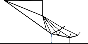
Figure 5 displays the predicted positions (circles) of the incident shock and cut-streamlines on the Mach number contour lines by CFD, for  $M_{0}=4$,
  $\theta _{w}=35.82^{\circ }$ and
  $g=0.76$. In the solution of the model, we have tested various choices of
  ${\rm d}\theta _{R}$ and we find the results with
  ${\rm d}\theta _{R}=0.01^{\circ }$ and
  ${\rm d}\theta _{R}=0.04^{\circ }$ display no obvious differences. It is seen that theory agrees well with CFD results. Similar comparison is observed for other conditions. Table 1 displays a comparison of the coordinates of
  $G$ and the shock angle
  $\beta _{G}$ at point
  $G$, for four sets of conditions. Note that the shock angle
  $\beta _{G}$ can only be measured approximately from CFD contour lines of Mach number or pressure. We have an error near
  ${\pm }0.5^{\circ }$ in measuring the shock angle.

Figure 5. Shape of the incident shock wave by CFD and theory. Open circles correspond to  ${\rm d}\theta _{R}=0.01^{\circ }$ and filled circles to
  ${\rm d}\theta _{R}=0.04^{\circ }$.
Table 1. Comparison of the coordinates of  $G$ and
  $\beta _{G}$ by theory (The) and CFD.

2.3. Transition criteria
The use of the algorithm in § 2.2 gives the shock angle  $\beta _{G}$ at the reflecting surface, which is used here as the input shock angle for the usual von Neumann condition and detachment condition of transition. Specifically, for any given set of
  $M_{0}$ and
  $\theta _{w}$, we find the value of
  $g$ at which the shock angle
  $\beta _{G}$ is equal to the usual von Neumann condition
  $\beta _{G}=$
  $\beta _{01}^{(N)}(M_{0})$ and the critical value of
  $g$ is denoted
  $g^{(N)}=g^{(N)}(M_{0},\theta _{w})$. We also find the critical value of
  $g$ such that
  $\beta _{G}$ is equal to the usual detachment condition
  $\beta _{G}=$
  $\beta _{01}^{(D)}(M_{0})$ and this critical
  $g$ is denoted
  $g^{(D)}=g^{(D)}(M_{0},\theta _{w})$. These critical conditions are displayed in figure 6, in terms of contour lines (iso-value lines) in the
  $M_{0}$–
 $\theta _{w}$ plane. The usual transition criteria in the case of a free incident shock wave are also displayed.

Figure 6. Critical conditions in the  $M_{0}$–
 $\theta _{w}$ plane: (a) the von Neumann condition
  $g=g^{(N)}$ and (b) the detachment condition
  $g=g^{(D)}$.
For any  $M_{0}$ and
  $\theta _{w}$ above the usual von Neumann condition, if
  $g< g^{(N)}(M_{0},\theta _{w})$, we may have a double solution or pure Mach reflection, and if
  $g>g^{(N)}(M_{0},\theta _{w})$, only regular reflection is possible. For fixed
  $\theta _{w}$, the critical value
  $g^{(N)}$ decreases when
  $M_{0}$ increases, meaning that transition from MR to RR occurs at smaller
  $g$ when
  $M_{0}$ increases. In contrast, for fixed
  $M_{0}$, increasing
  $\theta _{w}$ also increases
  $g^{(N)}$, meaning that transition from MR to RR occurs at larger
  $g$ when
  $\theta _{w}$ increases. For any
  $M_{0}$ and
  $\theta _{w}$ above the usual detachment condition, if
  $g>g^{(D)}(M_{0},\theta _{w})$, we are in the double solution domain or in the pure RR domain, and if
  $g< g^{(D)}(M_{0},\theta _{w})$, only Mach reflection is possible. Similarly as for the von Neumann condition, for fixed
  $\theta _{w}$,
  $g^{(D)}$ decreases when
  $M_{0}$ increases and, for fixed
  $M_{0}$, increasing
  $\theta _{w}$ also increases
  $g^{(D)}$.
Since  $g^{(N)}<1$, there is always a value of
  $g$ above which Mach reflection will transit to regular reflection, due to interaction between the TE expansion fan and the incident shock.
Another way to see the influence of  $g$ is to look at the transition criteria in the
  $g$–
$g$– $\theta _{w}$ plane for fixed
  $M_{0}$, as shown in figures 7(a) and 7(b) for
  $M_{0}=4$ and
  $6$. Line
  $CD$ is the detachment condition and line
  $AB$ is the von Neumann condition. The lines
  $D'CD$ and
  $B'AB$ enclose the double solution domain where both reflections are possible.

Figure 7. Transition criteria in the  $g$–
$g$– $\theta _{w}$ plane: (a)
  $M_{0}=4$ and (b)
  $M_{0}=6$.
Now we provide some numerical evidence on the influence of  $g$ on transition. Note that this is not a hysteresis study, but a study to show whether we can have MR or RR or both. In the dual solution, caution should be exercised in setting the initial condition; see Appendix A.1.
First, consider the condition with  $M_{0}=4$ and
  $\theta _{w}=30^{\circ }$, which is above the usual detachment condition, so we must have Mach reflection for small
  $g$. Now consider a large value
  $g=0.69$ for which we should have a double solution due to interaction, according to figure 7(a). We indeed have double solutions according to the numerical results displayed in figure 8(a) for RR and figure 8(b) for MR. For
  $g=0.75$, we obtain similar results, according to numerical solutions not shown here.

Figure 8. Mach contours showing double solution for  $M_{0}=4$ and
  $\theta _{w}=30^{\circ }$: (a) RR with
  $g=0.69$ and (b) MR with
  $g=0.69$.
The transition from MR to RR due to increasing  $g$ can also be seen from the numerical results of Mach stem height variation versus
  $g$, as shown in figure 9(a) for
  $M_{0}=4$ and
  $\theta _{w}=25^{\circ }$ (double solution domain in the case of free reflection) and figure 9(b) for
  $M_{0}=4$ and
  $\theta _{w}=30^{\circ }$ (pure Mach reflection domain in the case of free reflection). Hornung & Robinson (Reference Hornung and Robinson1982) used such a variation to demonstrate transition due to increase of wedge angle. Filled circles represent the Mach stem heights when the Mach reflection solution can be obtained and open circles, for zero Mach stem height, mean that regular reflection can be obtained by numerical solution. In the pure Mach reflection domain, we only have filled circles. In the pure regular reflection domain, we only have open circles. If, for the same value of
  $g$, we have both types of circles, then we are in the double solution domain.

Figure 9. Numerical results for normalized Mach stem heights as a function of the normalized wedge trailing-edge height for  $M_{0}=4$: (a)
  $\theta _{w}=25^{\circ }$ and (b)
  $\theta _{w}=30^{\circ }$.
For the case shown in figure 9(a), we have been able to produce regular reflection in all cases. Numerically, the transition from Mach reflection to regular reflection corresponds to  $g\approx 0.725$, while, according to figure 7(a), the theoretical transition condition is
  $g=g^{(N)}=0.731$ (represented by line
  $L$); thus the theoretical value
  $g^{(N)}$ is close to the CFD value. For the case shown in figure 9(b), where
  $L_{1}$ and
  $L_{2}$ represent, respectively, the theoretically predicted detachment condition
  $g^{(D)}=0.6868$ and the von Neumann condition
  $g^{(N)}=0.7668$, we observe that these theoretical values are very close to the CFD prediction.
Recall that the Mach stem height  ${H_{t}}/{H_{0}}$ decreases almost linearly with
  $g$, according to previous studies (Vuillon et al. Reference Vuillon, Zeitoun and Ben-Dor1995; Li & Ben-Dor Reference Li and Ben-Dor1997; Bai & Wu Reference Bai and Wu2021). Let
  $g_{v}$ be the value of
  $g$ at which the extended line of this linear curve intersects the
  $g$ axis (see figure 9). Owing to interaction, MR to RR transition occurs at
  $g=g^{(N)}$, not at
  $g=g_{v}$. Thus the quantity
  $g_{d}=g^{(N)}-g_{v}$ may measure indirectly the effect of transition delay due to interaction. Here
  $g_{v}$ can be obtained using the data by CFD for free Mach reflection. We get
  $g_{v}\approx 0.7665$,
  $g^{(N)}\approx 0.8$ and
  $g_{d}\approx 0.034$ for
  $M_{0}=3$ and
  $\theta _{w}=25^{\circ }$, we get
  $g_{v}\approx 0.7$,
  $g^{(N)} \approx 0.722$ and
  $g_{d}\approx 0.022$ for
  $M_{0}=4$ and
  $\theta _{w}=25^{\circ }$, and we get
  $g_{v}\approx 0.717$,
  $g^{(N)}\approx 0.76$ and
  $g_{d}\approx 0.043$ for
  $M_{0}=4$ and
  $\theta _{w}=30^{\circ }$.
Recall that transition from MR to RR for large  $g$ has been observed numerically by Vuillon et al. (Reference Vuillon, Zeitoun and Ben-Dor1995) and Li & Ben-Dor (Reference Li and Ben-Dor1997) for some particular conditions. Here we have obtained the threshold of
  $g$ for transition for a wide parameter range.
3. Mach reflection with interaction
3.1. Wave structure in Mach reflection with interaction
The secondary waves generated over the slipline due to reflection of transmitted expansion waves and due to equilibrium of pressures across the slipline have been found to have an important effect on the shape and size of free Mach reflection (Gao & Wu Reference Gao and Wu2010; Bai & Wu Reference Bai and Wu2017). Here the problem is more pronounced since secondary waves and shear layers are also generated from reflection of expansion waves over the incident shock. Thus, it is important to clarify the wave structures.
The wave structure can be made clear if we show both contour lines and characteristics. See Appendix A.1 for the method to display the characteristic lines. In figures 10(a) and 10(b) we display the contour lines of the Mach number  $M$ and pressure
  $p$, superimposed by characteristic lines, obtained by numerical simulation with
  $M_{0}=4$,
  $\theta _{w}=30^{\circ }$ and
  $g=0.7$. Figure 11 is a schematic display of the various waves depicted following figure 10. Now we describe the particular features of the various waves, shear layers and the flow structures typical of Mach reflection with interaction.

Figure 10. Numerical solution of Mach reflection for  $M_{0}=4$,
  $\theta _{w}=30^{\circ }$ and
  $g=0.7$: (a) Mach number contours and characteristic lines, and (b) pressure contours and characteristic lines. The characteristic lines are displayed as solid lines and the contour lines as dashed lines.

Figure 11. Schematic display of wave patterns for Mach reflection. The three families of characteristics are displayed in various types of curves.
(a) Mach waves from the TE expansion fan (belonging to  $C_-$). According to figure 10, these waves have small curvature, a property that justifies the approximation (A8) and similar approximation used in Appendix A.3. Below the cut-streamline, the Mach contour lines are not aligned with the characteristics lines
  $C_-$ so that the Mach number is not constant along
  $C_-$, while the pressure and also the flow deflection angle
  $\theta$ according to numerical results not shown here are nearly constant along
  $C_-$ (a property to be used in Appendix A.3 for the upstream condition of the reflected shock).
(b) Reflected Mach waves from the incident shock (belonging to  $C_+$). The reflected Mach waves (cf.
  $i_{2}r_{1}$) from the incident shock (part
  $i_{0}i_{1}i_{2}T$) disturb the expansion fan above the cut-streamline. These reflected Mach waves are one order of magnitude weaker than the incoming Mach waves, according to Guan, Bai & Wu (Reference Guan, Bai and Wu2020, figure 6) for a similar problem, and thus their influence may be neglected in a first-order approximation.
(c) Shear layers from the incident shock (belonging to  $C_{0}$). These characteristics
  $C_{0}$ (like
  $i_{1}r_{1}$) are along the streamlines. Figure 10(a) shows that the Mach number contour lines are highly distorted below the cut-streamline
  $i_{0}r_{2}$ shown in figure 11. Thus the influence of these shear layers on the reflected shock cannot be neglected (see Appendix A.3 for how to model this interaction).
(d) Three types of incoming waves upstream of the reflected shock. Consider a typical point  $r_{1}$ on the reflected shock. There are three waves coming from upstream of this point: the wave
  $i_{3}^{C_{0}}r_{1}$ (
 $C_-$) comes from R, the wave
  $i_{1}r_{1}$ (
 $C_{0}$) comes from the incident shock, and the wave
  $i_{2}r_{1}$ (
 $C_+$) is a reflected Mach wave from the incident shock. These waves alter the upstream condition of the reflected shock. As discussed above,
  $i_{3}^{C_{0}}r_{1}$ and
  $i_{1}r_{1}$ cannot be neglected but
  $i_{2}r_{1}$ can be omitted.
(e) Waves over the slipline. The transmitted Mach waves (such as  $r_{1}s_{3}$) belonging to
  $C_-$ are reflected over the slipline to produce Mach waves (cf.
  $s_{3}r_{6}$) belonging to
  $C_+$.
(f) Waves downstream of the reflected shock. Apart from the transmitted Mach waves (like  $r_{1}s_{3}$) and characteristics belonging to
  $C_{0}$ (like
  $r_{1}o$), reflected waves from the slipline (like
  $s_{1}r_{1}$) appear downstream of the reflected shock and may change its shape. The strengths of these reflected waves can be measured by the variation of eigenvalues
  $\tan ( -\theta \pm \mu )$ along the slipline. Figure 12 displays
  $\tan ( -\theta \pm \mu )$ for
  $M_{0}=4$,
  $\theta _{w}=30^{\circ }$ and
  $g=0.7$, with
  $\theta$ and
  $\mu$ obtained from CFD. The variation of
  $\tan ( -\theta +\mu )$ for the reflected wave is much smaller than
  $\tan (-\theta -\mu )$ for the transmitted wave. Similar results are observed for
  $g=0.675$ and
  $0.7$. Thus, the reflected Mach waves from the slipline are weak and its influence on the shape of the reflected shock can be neglected, like in previous studies of free Mach reflection.

Figure 12. Slopes of the characteristics  $C_-$ and
  $C_+$ along the slipline for
  $M_{0}=4$,
  $\theta _{w}=30^{\circ }$ and
  $g=0.7$.
In summary, the overall flow configurations are highly disturbed by Mach waves and shear layers generated by interaction between the TE expansion fan and the incident shock. Not only is the upstream condition of the reflected shock perturbed by three families of waves, one from the wedge corner, but also the transmitted expansion waves are perturbed by shear layers from the incident shock.
3.2. Modelling of the Mach reflection configuration
In his monograph, Ben-Dor (Reference Ben-Dor2007) stated that the mechanism by which the size of the entire wave configuration of the MR was determined has been considered as an important issue; see also Ben-Dor & Takayama (Reference Ben-Dor and Takayama1992) for the importance of this. Hornung & Robinson (Reference Hornung and Robinson1982) argued that the Mach stem height is affected by the pressure decreasing information from the wedge TE expansion fan, since this information can be carried out to the subsonic flow region in the quasi-one-dimensional flow region below the slipline and then transported upstream to the triple point through the subsonic pocket. As a result, the size and shape of this subsonic pocket are controlled by the distance between the Mach stem and the sonic throat, which in turn depends on the geometry of the wedge and the relative height ( $g$) of the trailing edge.
Since then, theoretical modelling of the Mach stem height for free Mach reflection has been attempted a number of times: see, for instance, Azevedo & Liu (Reference Azevedo and Liu1993), Li & Ben-Dor (Reference Li and Ben-Dor1997), Mouton & Hornung (Reference Mouton and Hornung2007), Gao & Wu (Reference Gao and Wu2010) and Bai & Wu (Reference Bai and Wu2017) for planar two-dimensional shock reflection, and Shoesmith & Timofeev (Reference Shoesmith and Timofeev2021) for axisymmetrical shock reflection. It remains to consider Mach reflection with interaction. Though modern CFD can predict the details for each given condition, a very fine grid is needed to capture the height of the Mach stem, as shown in Appendix A.1. So it is better to use CFD and theoretical modelling in a combined way if we want to study the Mach stem height for a wide range of parameters.
The wave pattern used for modelling is shown in figure 13, accounting for the various waves and shear layers shown in figure 11. As usual, the perturbation of the reflected waves from the slipline on the downstream condition of the reflected shock is not accounted for. The modelling given below is based on that given by Bai & Wu (Reference Bai and Wu2017) for free reflection, accounting for the particular features due to interaction. The detailed algorithm is given in Appendices A.2–A.5; below, we only summarize the particular features due to interaction.

Figure 13. Notations for wave structure used for model construction.
The first particular feature is that the triple-point solution is coupled with the global solution, unlike in free Mach reflection where the triple-point solution only depends on the inflow condition and the wedge angle. Thus, the triple-point solution is determined in a coupled way with the Mach stem height model and the incident shock shape model. For each temporal height of the Mach stem, the shape of the incident shock is solved up to the triple point, using the method given in Appendix A.2 which gives the shock angle  $\beta _{01}^{(T)}$ at the assumed triple-point location. The conventional triple-point theory of von Neumann is then used to find
  $\beta _{12}^{(T)}$,
  $\beta _{03}^{(T)}$,
  $\theta _{2}^{(T)}$,
  $\theta _{s}^{(T)}$,
  $M_{k}^{(T)}$,
  $\rho _{k}^{(T)}$ and
  $p_{k}^{(T)}$ (
 $k=1,2,3$).
The second particular feature is that the upstream flow conditions of the reflected shock are subjected to the influence of waves and shear layers produced over the incident shock (see  $Rf$,
$Rf$,  $Qf$ and
  $Q^{\prime }f$ for each point on the incident shock, as shown in figure 13), unlike free Mach reflection for which the upstream condition of the reflected shock is determined uniquely by the TE expansion fan. This requires the consideration of three families of characteristics, to bring information from the wedge trailing edge and from the curved incident shock.
There are also particular features associated with the shape of the reflected shock, the transmitted expansion waves and the shape of the slipline, noting that modelling these shapes is already very difficult in free Mach reflection. Like in free Mach reflection, the shape of the reflected shock and its downstream flow conditions are determined by conventional type I interaction between Mach waves and shock wave (Bai & Wu Reference Bai and Wu2017), but with far more complicated upstream flow conditions (determined in Appendix A.3) for the reflected shock segment  $TF$. Unlike in free Mach reflection, where the transmitted Mach waves are usually treated as straight lines and the pressure is assumed to be constant along the transmitted Mach waves (Li & Ben-Dor Reference Li and Ben-Dor1997; Bai & Wu Reference Bai and Wu2017), here, due to the oncoming waves and shear layers from the incident shock, the characteristics should be regarded as curved lines and the pressure should be determined by the compatibility relation (outlined in Appendix A.1). The model for the shape of the slipline does not have new features compared to free Mach reflection. The algorithm is outlined in Appendix A.4.
The global algorithm for the Mach stem height and for the shape of the reflected shock and slipline, outlined in Appendix A.5, is similar to that for free Mach reflection, except that, as stated above, the triple-point solution is coupled with the estimated value of the Mach stem height, which again depends on the triple-point solution, the shape of the reflected shock and the shape of the slipline. Thus, the global algorithm for the Mach stem height is more complex than in free Mach reflection.
Figure 14 shows Mach stem heights as a function of  $g$, obtained by both prediction and CFD, for three sets of
  $M_{0}$ and
  $\theta _{w}$:
  $M_{0}=3$,
  $\theta _{w}=25^{\circ }$;
  $M_{0}=4$,
  $\theta _{w}=25^{\circ }$; and
  $M_{0}=4$,
  $\theta _{w}=30^{\circ }$. The theory predicts a Mach stem height slightly higher than CFD in all cases but the absolute errors reduce for larger
  $g$. In free Mach reflection, similar amounts of errors also exist due to simplifications needed in a solvable model (Azevedo & Liu Reference Azevedo and Liu1993; Li & Ben-Dor Reference Li and Ben-Dor1997; Mouton & Hornung Reference Mouton and Hornung2007; Gao & Wu Reference Gao and Wu2010).

Figure 14. Mach stem heights as functions of  $g$ for three sets of
  $M_{0}$ and
  $\theta _{w}$.
Figure 15 overlaps the shape of the slipline, incident shock and reflected shock predicted by theory on the Mach number contour lines by CFD, for  $M_{0}=4$,
  $\theta _{w}=30^{\circ }$ and two
  $g$ values, showing how the theory agrees with CFD.

Figure 15. Shapes of incident shock, reflected shock and slipline for  $M_{0}=4$,
  $\theta _{w}=30^{\circ }$ and (a)
  $g=0.7$ or (b)
  $g=0.73$.
3.3. Influence of interaction on the Mach reflection configuration
The influence of interaction on the overall wave configuration for a typical value of  $g$ has been discussed in § 3.1. One point to be emphasized again is that the flow below the cut-streamline (especially the Mach number according to figure 10a) is highly perturbed by the waves and shear layers produced over the incident shock.
According to a number of numerical results, the overall wave pattern is similar for various values of  $g$, except that the cut-streamline and the critical characteristic line (the characteristic line of the expansion fan joining the sonic throat, see Bai & Wu (Reference Bai and Wu2021)) may intersect at a point upstream or downstream of the reflected shock. Figure 16 shows, for
  $M_{0}=4$ and
  $\theta _{w}=30^{\circ }$, that these two lines intersect at a point upstream of the reflected shock when
  $g=0.7$, and downstream when
  $g=0.73$. These two possibilities should be considered in the solution of the Mach stem model, since the flow should be solved up to the critical characteristic line in the Mach reflection model (see Appendix A.5).

Figure 16. Relative positions of  $F$ and
  $f$ marked on Mach number contours for
  $M_{0}=4$,
  $\theta _{w}=30^{\circ }$ and (a)
  $g=0.7$ or (b)
  $g=0.73$.
The Mach stem height is an important parameter that characterizes the Mach reflection configuration, as mentioned at the beginning of § 3.2. For the present problem with interaction, the value of  $g$ at which interaction occurs is also of interest (note that, for regular reflection, this condition has been given in figure 4). We consider how the Mach stem height varies with
  $M_{0}$ and
  $\theta _{w}$ when interaction occurs, and how the Mach stem height depends on
  $g$. Figures 17(a) and 17(b) display the curve
  ${H_{t}}/{H_{0}}=f(g)$ for various choices of
  $\theta _{w}$ and
  $M_{0}$.

Figure 17. Mach stem heights as a function of the normalized wedge trailing-edge height: (a)  $M_{0}=4$ and five
  $\theta _{w}$; and (b)
  $\theta _{w}=25^{\circ }$ and four
  $M_{0}$.
As in the three cases shown in figure 14, for each set of  $\theta _{w}$ and
  $M_{0}$,
  ${H_{t}}/{H_{0}}$ decreases nonlinearly with
  $g$, much more slowly than the linear decrease observed in free reflection (Vuillon et al. Reference Vuillon, Zeitoun and Ben-Dor1995; Li & Ben-Dor Reference Li and Ben-Dor1997; Bai & Wu Reference Bai and Wu2021). In both figures 17(a) and 17(b), the starting abscissa
  $g=g_{s}$ (marked with a dot) for each curve is the point where the leading characteristic line of the wedge TE expansion fan intersects the triple point.
According to figure 17(a), which shows  ${H_{t}}/{H_{0}}=f(g)$ with
  $M_{0}$ fixed to
  $4$ and with various
  $\theta _{w}$, the Mach stem is higher for larger
  $\theta _{w}$. The same trend has been observed in free Mach reflection (Hornung & Robinson Reference Hornung and Robinson1982). According to figure 17(a), which shows
  ${H_{t}}/{H_{0}}=f(g)$ with
  $\theta _{w}$ fixed to
  $25^{\circ }$ and with various
  $M_{0}$, the Mach stem is higher for smaller
  $M_{0}$. The same trend has been observed in free Mach reflection (Gao & Wu Reference Gao and Wu2010).
The location  $g_{s}$ of the starting point of interaction is found to be monotonically decreasing when
  $M_{0}$ increases, according to figure 17(b). However, when
  $M_{0}$ is fixed to be
  $4$, the smallest value of
  $g_{s}$ occurs at
  $\theta _{w}$ around
  $28^{\circ }$. For larger and smaller
  $\theta _{w}$,
  $g_{s}$ takes larger values. The width
 \begin{equation} g_{i}=g^{(N)}-g_{s} \end{equation}
is the interval of  $g$ over which interaction occurs. It is the width of
  $g$ over which the Mach stem vanishes from the beginning of interaction. According to figure 17(a), for larger
  $\theta _{w}$, the Mach stem height is larger, and requires a wider interval
  $g_{i}$ for vanishing Mach stem height. However, according to figure 17(b), for smaller
  $M_{0}$, though the Mach stem height is larger, it requires a shorter interval
  $g_{i}$ for vanishing Mach stem height. Consider, for instance,
  $M_{0}=3$ and
  $\theta _{w}=25^{\circ }$: interaction starts at
  $g=g_{s}\approx 0.73$ and the Mach stem height vanishes at
  $g=g^{(N)}\approx 0.8$, so
  $g_{i}\approx 0.07$; while for
  $M_{0}=5$ and
  $\theta _{w}=25^{\circ }$, interaction starts at
  $g=g_{s}\approx 0.624$ and the Mach stem height vanishes at
  $g=g^{(N)}\approx 0.7$ so
  $g_{i}\approx 0.076$.
Note that, for low enough  $g$, the flow will not start or will ‘unstart’ if the reflected shock intersects the wedge lower surface before the trailing edge, according to Li & Ben-Dor (Reference Li and Ben-Dor1997, figures 7 and 8). In the present paper, we are interested in high
  $g$, and the ‘unstart’ problem is not encountered for the range of
  $g$ we have studied.
4. Conclusion
In this paper we have studied the influence of the interaction between the trailing-edge (TE) expansion fan and the incident shock wave on both regular reflection (RR) and Mach reflection (MR), including on the transition criteria and on the Mach reflection configuration. This influence is parametrized in terms of  $g$, the wedge trailing-edge height divided by the inlet height.
It is shown that the parameter range for interaction is large, especially for large Mach number, where interaction may occur for small  $g$ (see figure 4). The von Neumann condition and detachment condition are displayed in the
  $M_{0}$–
 $\theta _{w}$ plane for various values of
  $g$ (see figure 6). These results quantify the effect of
  $g$ on transition delay due to interaction, and complement the previous work of Vuillon et al. (Reference Vuillon, Zeitoun and Ben-Dor1995) and Li & Ben-Dor (Reference Li and Ben-Dor1997), who first pointed out the possibility that MR to RR transition would occur for large enough
  $g$.
$g$.
Through the display of the characteristics of various families, the complex waves and shear layers embedded in the overall Mach reflection configuration are clarified. The particular features from interaction in the mechanism by which the size and shape of the overall flow configuration are determined are discussed. The inclusion of the particular features into a previous Mach reflection model (for free reflection) gives a Mach stem height model capable of accounting for the interaction and predicting the Mach stem height for a wide range of  $g$. It is found that the relative Mach stem height decreases nonlinearly with increasing
  $g$ for Mach reflection with interaction. This is in contrast to free Mach reflection, where this height decreases almost linearly with
  $g$ according to previous studies (Vuillon et al. Reference Vuillon, Zeitoun and Ben-Dor1995; Li & Ben-Dor Reference Li and Ben-Dor1997; Bai & Wu Reference Bai and Wu2021). Meanwhile, even with interaction, the relative Mach stem height increases with
  $\theta _{w}$ and decreases with
  $M_{0}$ if the other parameters are fixed, as in free reflection. The expansion fan interacts with the incident shock before the triple point at
  $g=g_{s}$, where
  $g_{s}$ is monotonically decreasing when
  $M_{0}$ increases when
  $\theta _{w}$ is fixed, while
  $g_{s}$ is not monotonic with
  $\theta _{w}$ for
  $M_{0}$ fixed, at least for the parameters considered. The interval of
  $g$ over which the Mach stem vanishes starting from interaction is also found to depend on
  $\theta _{w}$ and
  $M_{0}$.
Acknowledgements
The author is grateful to all referees for their valuable comments and suggestions, which helped to complete and improve this work.
Funding
This work was supported by the Young Elite Scientist Sponsorship Program by CAST (No. YESS20210042), the National Natural Science Foundation of China (No. 52192632 and 11721202), National Key Project GJXM92579 and the Young Talent Support Plan of Beihang University.
Declaration of interests
The author reports no conflict of interest.
Appendix A. Numerical and analytical modelling
A.1. Basic flow models, approximate characteristics method and numerical simulation
The present study considers only two-dimensional inviscid flow of a perfect gas, with a specific heat ratio  $\gamma$ (
 $=1.4$ for air). As convention, the Mach number is denoted as
  $M$, the pressure as
  $p$, density as
  $\rho$, the Mach angle as
  $\mu$ (
 $=\arcsin (1/M)$), the local shock angle as
  $\beta$ and the local flow deflection angle as
  $\theta$. The upstream supersonic flow is set to be horizontal, and the angle
  $\theta$ is with respect to the horizontal direction and assumed to be positive when the flow deflects towards the reflecting surface.
Throughout this paper, the shock angle relation is abbreviated as  $\vert \theta ^{(u)}-\theta ^{(d)} \vert = f_{\theta }(M^{(u)},\beta )$, and the oblique shock-wave relations are abbreviated as
  $p^{(d)}=p^{(u)}\,f_{p}(M^{(u)},\beta )$ and
  $M^{(d)}=f_{M}(M^{(u)},\beta$), where the superscripts
  $(u)$ and
  $(d)$ mean upstream and downstream. The expressions
  $f_{\theta } (M,\beta )$,
  $f_{p}(M,\beta )$ and
  $f_{M}(M,\beta$) can be found in any classic textbook for gas dynamics. The abbreviation
  $\vartheta (M) = [1+\tfrac {1}{2}(\gamma -1)M^{2}]^{\gamma /(\gamma -1)}$ that arises from isentropic flow relations is also used.
There are three families of characteristics,  $C_-$,
  $C_{0}$ and
  $C_+$. Along the characteristic lines
  ${{\rm d}y}/{{\rm d}\kern0.06em x}=\tan ( -\theta \mp \mu )$ belonging to
  $C_-$ and
  $C_+$ the following compatibility relations hold (cf. Holt Reference Holt1956; Liepmann & Roshko Reference Liepmann and Roshko1957; Hayes & Probstein Reference Hayes and Probstein2004):
 \begin{equation} -{\rm d}\theta \mp \varPhi (\,p,M){\rm d}p=0,\quad \varPhi (\,p,M)=\frac{\sqrt{M^{2}-1}}{\gamma M^{2}p} \quad (C_{{\mp}}). \end{equation}
Along the characteristic line  ${{\rm d}y}/{{\rm d}\kern0.06em x}=\tan ( -\theta )$ belonging to
  $C_{0}$, the following holds:
 \begin{equation} {\rm d}p-a^{2}{\rm d}\rho =0, \quad \rho V{\rm d}V+{\rm d}p=0 \quad (C_{0}). \end{equation}
We will see that some characteristic lines have small differences in their slopes at their two ends, so the approximation of Li & Ben-Dor (Reference Li and Ben-Dor1997) can be applied to these characteristic lines, giving
 \begin{equation} y_{2}-y_{1}=(x_{2}-x_{1})\tan \varLambda (\delta _{1},\delta _{2}), \end{equation}
where  $\delta _{1}$ and
  $\delta _{2}$ are the slopes at the two end points
  $1$ and
  $2$, and
 \begin{equation} \varLambda (\delta _{1},\delta _{2}) =\arctan\frac{2\tan \delta _{1}+\tan (\delta _{2}-\delta _{1})} {2-\tan \delta _{1}\tan (\delta _{2}-\delta _{1})}. \end{equation}
 Tecplot can draw streamlines, with velocity components as input. This streamline function is used to draw the characteristic lines  ${{\rm d}y}/{{\rm d}\kern0.06em x} =\tan ( -\theta \mp \mu )$, by using
  $(1,\tan ( -\theta \pm \mu ) )$ as the fictive velocity (
 $\theta \pm \mu$ are from the CFD solution).
The CFD results are obtained by solving the compressible Euler equations for a perfect gas (air) using the well-known second-order Roe scheme, on a structured grid. The inlet is supersonic, the reflecting surface is symmetric, the wedge lower surface is an inviscid wall, the upper boundary downstream of the wedge is also an inviscid wall, and the exit is a supersonic outlet. For Mach reflection simulations, the exit is sufficiently far downstream so that the exit flow (in the streamtube downstream of the Mach stem) is supersonic. As usual, an unsteady approach is used to converge to the steady-state solution, so we need an initial condition. A uniform initial condition with the flow parameters set to the inlet values is used, which is found to give RR in the RR domain, and MR in the MR domain. Caution should be taken in the dual solution domain, if one wants to produce RR in one computation and MR in another. If we want to display that a numerical solution with RR is possible, then a uniform initial condition is given. If we want to demonstrate that a numerical solution with MR is possible, then the initial condition can be set as the converged numerical solution corresponding to a smaller inflow Mach number above the detachment condition.
To see how the numerical results are dependent on the grid density, we consider  $M_{0}=4$,
  $\theta _{w}=30^{\circ }$ and
  $g=0.675$ and test four grids: grid A has
  $380\times 180$ points, grid B has
  $760\times 360$ points, grid C has
  $1520\times 720$ points, and grid D has
  $2280\times 1080$ points. A grid density like grid A has been considered suitable for Mach stem height study without interaction (cf. Gao & Wu Reference Gao and Wu2010). Below, we will see that this is not the case when there is interaction.
The role of grid density is seen from the Mach stem heights. Table 2 displays the Mach stem heights on the four grids. It is seen that the Mach stem heights with grids C and D are very close, so the solution with grid D may be considered as a reference result. Compared to this reference result, grid A has an error close to 19 %, and for grid B, which is two times finer than grid A, the error is reduced almost two times. Grid C, which is two times finer than grid B, has an error of about 2 %.
Table 2. Mach stem heights for various grid densities.

In summary, the grid density usually used for free Mach reflection has a large error for the present problem with interaction. A much finer grid, like grid C or grid D, should be used for accurate prediction. In this paper, we will use a grid as dense as grid C. Moreover, along the Mach stem we use  $80$ points between the reflecting surface and the triple point, to resolve the Mach stem. The total number of grid points in the vertical direction is about
  $1000$.
A.2. An algorithm for the shape of the incident shock
Consider a typical characteristic  $RQ$ as shown in figure 3. Point
  $P$ also is on the cut-streamline that separates the TE expansion fan into an upper region and a lower region. According to figure 2(a), the Mach number inside the TE expansion fan is seriously perturbed by interaction only in this lower region. Thus the characteristics in the upper region can be treated as simple waves and those in the lower region can be treated using the method of characteristics for rotational flow. To do this, we first need the shape of the cut-streamline. Note that Liepmann & Roshko (Reference Liepmann and Roshko1957) asked readers to do a homework exercise to find this shape, and the algorithm given below would be different from what they envisaged.
For a variation  ${\rm d}\theta _{R}$ of the flow deflection angle
  $\theta _{R}$ inside the TE expansion fan, starting from
  $\theta _{w}$, the variations of the parameters
  $M_{R}$,
  $p_{R}$ and
  $\rho _{R}$ are obtained from the well-known isentropic Mach wave relations, which can be found in classical textbooks for gas dynamics. The coordinates of
  $P$, with
  $\theta _{P}=\theta _{R}$, on the cut-streamline are then solved using
 \begin{equation} \left\{\begin{array}{@{}l} \dfrac{{\rm d}y_{P}}{{\rm d}\kern0.06em x_{P}}=-\tan \theta _{P} \quad (P\ \text{is on the streamline}), \\ y_{P}-y_{R}=-(x_{P}-x_{R})\tan ( \theta _{P}+\mu _{P})\quad (P\ \text{is on PR}), \end{array}\right. \end{equation}
where  $\mu _{P}=\sin ({1}/{M_{P}})$ with
  $M_{P}$ related to
  $\theta _{P}$ through the Prandtl–Meyer relation
  $\nu (M_{P})-\nu (M_{{1}})=\theta _{{w}}-\theta _{P}$,
  $\nu (M)$ being the well-known Prandtl–Meyer function.
The coordinates of  $Q$ are related to the shock angle
  $\beta _{Q}$ by
  ${\rm d} y_{Q}=-\tan \beta _{Q} \, {\rm d}\kern0.06em x_{Q}$, where
  $\beta _{Q}$ is the shock angle at point
  $Q$. To determine
  $\beta _{Q}$ we need the downstream flow conditions at point
  $Q$. The required downstream conditions here are the pressure
  $p_{Q}$ and the flow deflection angle
  $\theta _{Q}$, which will be related to the pressure
  $p_{P}$ and flow deflection angle
  $\theta _{P}$ using the relations along the characteristic
  $PQ$. According to figure 2(a) and according to the numerical result for
  $\theta$ not shown here, both
  $p$ and
  $\theta$ have little variation along
  $PQ$, so that the first-order approximation
 \begin{equation} \theta _{P}-\theta _{Q}=\varPhi _{{SQ}} ( \,p_{Q}-p_{P} ) \end{equation}
can be used to approximate the compatibility relation for  $C_-$ (see (A1a,b)). Here,
  $\varPhi _{{SQ}}$ can be approximated by using the averaged values at points
  $P$ and
  $Q$. The use of the oblique shock relations gives another expression for
  $\theta _{Q}$ and
  $p_{Q}$:
 \begin{equation} p_{Q}=p_{0}\,f_{p}(M_{0},\beta _{Q}), \quad \theta _{Q}=f_{\beta }(M_{0},\beta _{Q}). \end{equation}
 For any given  $\theta _{P}=\theta _{R}$, expressions (A6) and (A7) define a closed set of relations for
  $\theta _{Q}$,
  $\beta _{Q}$ and
  $p_{Q}$. The density and Mach number at point
  $Q$ are then computed as
  $\rho _{Q}= \rho _{0}\,f_{\rho }(M_{0},\beta _{Q})$ and
  $M_{Q}=f_{M}(M_{0},\beta _{Q})$. The Mach angle is computed as
  $\mu _{Q}=\arcsin M_{Q}^{-1}$.
The coordinates of  $Q$ are then related to the coordinates of
  $P$ through the characteristic line
  ${{\rm d}y}/{{\rm d}\kern0.06em x}=\tan \delta$, where
  $\delta =-\theta -\mu$ is the slope of
  $PQ$. Since the variation of this slope along
  $PQ$ is small according to figure 2, the second-order curve approximation (A3) is used to establish a relation between
  $P$ and
  $Q$, giving
 \begin{equation} y_{Q}-y_{P}=(x_{Q}-x_{P})\tan \varLambda (\delta _{1},\delta _{2}), \end{equation}
where  $\delta _{1}=-( \theta _{P}+\mu _{P})$ and
  $\delta _{2}=-( \theta _{Q}+\mu _{Q})$. Combining
  ${\rm d}y_{Q}=-\tan \beta _{Q}\,{\rm d}\kern0.06em x_{Q}$ and the differential form of (A8) gives
  ${\rm d}\kern0.06em x_{Q}=Z_{Q}$ and
  ${\rm d}y_{Q}=-Z_{Q}\tan \beta _{Q}$, where
 \begin{equation} Z_{Q}=\frac{\tan \varLambda \, {\rm d}\kern0.06em x_{P}-{\rm d}y_{P}-(x_{Q}-x_{P}) ( \varLambda _{\delta _{1}}{\rm d}\delta _{1} +\varLambda _{\delta 2}{\rm d}\delta _{2})\cos^{-2}\varLambda } { \tan \beta _{Q}+\tan \varLambda } . \end{equation}
Here,  $\varLambda _{\delta _{1}}$ and
  $\varLambda _{\delta 2}$ denote derivatives of
  $\varLambda$ with respect to
  $\delta _{1}$ and
  $\delta _{2}$.
Now we outline the algorithm for the shape of the incident shock. Let  $M_{0}$ and
  $\theta _{w}$ and
  $g$ be provided. Without loss of generality, we set
  $H_{A}=1$,
  $p_{0}=1$ and
  $\rho _{0}=1$. Then
  $h=gH_{A}=g$,
  $w={(H_{A}-h)}/{\sin \theta _{w}}$,
  $x_{R}=w\cos \theta _{w}$ and
  $y_{R}=h$. The parameters
  $\beta _{01}$,
  $M_{1}$,
  $p_{1}$ and
  $\rho _{1}$ in the unperturbed region (1) are obtained using the oblique shock-wave relations. Put
  $\mu _{1}=\arcsin ({1}/{M_{1})}$. Compute
  $x_{I}$ and
  $y_{I}$ (see (2.1a,b)).
Step 1. Start from  $\theta _{P}=\theta _{w}$, set
  $x_{Q}=x_{I}$,
  $y_{Q}=y_{I}$,
  $\theta _{Q}=\theta _{P}$,
  $M_{P}=M_{1}$,
  $p_{P}=p_{1}$,
  $\rho _{P}=\rho _{1}$ and
  $\mu _{P}=\mu _{Q}=\arcsin ({1}/{M_{1}})$.
Step 2. For any  $\theta _{P}=\theta _{P}+{\rm d}\theta _{P}$, first solve the isentropic Mach wave relations for
  $M_{P}$,
  $p_{P}$ and
  $\mu _{P}$ (and thus
  ${\rm d}\mu _{P}$), then use (A5) for
  $x_{P}$ and
  $y_{P}$.
Step 3. Solve (A6) and (A7) for  $\theta _{Q}$,
  $p_{Q}$ and
  $\beta _{Q}$ and use shock relations for
  $\rho _{Q}$ and
  $M_{Q}$.
Step 4. Solve  ${\rm d}\kern0.06em x_{Q}=Z_{Q}$ and
  ${\rm d}y_{Q}=-Z_{Q}\tan \beta _{Q}$ for
  ${\rm d}\kern0.06em x_{Q}$ and
  ${\rm d}y_{Q}$, and set
  $x_{Q}=x_{Q}+{\rm d}\kern0.06em x_{Q}$ and
  $y_{Q}=y_{Q}+{\rm d}y_{Q}$.
A.3. Method to find the upstream conditions of the reflected shock wave
Consider the upstream conditions of any point  $f$ on the reflected shock (see figure 13 for notation). The superscript
  $(u)$ is used to denote flow parameters just upstream of the reflected shock.
The upstream conditions are first linked to the conditions at point  $S$ through the compatibility relation along the characteristic line
  $Sf$ (which belongs to
  $C_-$), with
  $S=e$ if
  $f$ is on the left of
  $F$ and
  $S=R$ if
  $f$ is on the right of
  $F$. Like (A6), the compatibility relation for
  $Sf$ is approximated as
 \begin{equation} \theta _{f}^{(u)}-\theta _{S}=\varPhi _{{Sf}}(\,p_{S}-p_{f}^{(u)}), \end{equation}
which defines one relation for  $\theta _{f}^{(u)}$ and
  $p_{f}^{(u)}$. The upstream conditions are then linked to the conditions at point
  $Q$ on the incident shock, through the two compatibility relations (A2a,b) along the streamline
  $Qf$ (which belongs to
  $C_{0}$), and these two relations can be solved to give one relation for
  $M_{f}^{(u)}$ and
  $p_{f}^{(u)}$:
 \begin{equation} \vartheta (M_{f}^{(u)})^{{\gamma}/{(\gamma -1)}}p_{f}^{(u)}=\vartheta (M_{Q})^{{\gamma }/{(\gamma -1)}}{}p_{Q}. \end{equation}
 Though  $p_{Q}$ and
  $M_{Q}$ are known from the solution of the shape of the incident shock (Appendix A.2), a connection between the positions of point
  $f$ and point
  $Q$ is needed in order to apply (A11). Now we provide a simple way to make this connection. In an unperturbed expansion fan, the mass flux
  $q(\theta _{z})$ in a tube bounded by a streamline and the expansion corner is obviously constant. At any point
  $z$, with a distance
  $r_{z}$ to this corner, this mass flux is
 \begin{equation} q(\theta _{z})=\rho _{z}V_{z}r_{z}\sin \mu _{z}, \end{equation}
where  $\rho _{z}$,
  $V_{z}$ and
  $\mu _{z}$ are functions of
  $\theta =\theta _{z}$ according to the well-known Prandtl–Meyer relation.
Now, in the rotational flow region  $IFT$ shown in figure 13, the expansion fan is perturbed by the entropy layers and reflected waves from the segment
  $IT$ of the incident shock, so that (A12) no longer holds exactly. However, just to obtain a connection between points
  $f$ and
  $Q$, (A12) may be used as an approximation. The positions of points
  $f$ and
  $Q$, in terms of
  $\theta$, can then be connected through
  $q(\theta _{Q})=q(\theta _{f}^{(u)})$, where
  $q(\theta _{f}^{(u)})=\rho _{R}V_{R}r_{f}\sin \mu _{R}$. The value of
  $q(\theta _{Q})$ at any point
  $Q$ is then determined by
  $q(\theta _{Q})=q(\theta _{f}^{(u)})$. Since the values of
  $\rho _{Q}$,
  $p_{Q}$,
  $M_{Q}$,
  $\mu _{Q}$ and
  $r_{Q}$ at any point
  $\theta _{Q}$ have been solved in the algorithm for the shape of the incident shock, the value
  $\theta _{Q}$ can then be solved from
  $\rho _{Q}V_{Q}r_{Q}\sin \mu _{Q}=q(\theta _{Q})=q(\theta _{f}^{(u)})$.
Now we have just two expressions (A10) and (A11) for the three unknowns  $M_{f}^{(u)}$,
  $p_{f}^{(u)}$ and
  $\theta _{f}^{(u)}$. If
  $S$ is
  $R$, then we set
  $p_{S}=p_{R}$ and
  $\theta _{S}=\theta _{R}$ and use (A11) for
  $M_{f}^{(u)}$. For the case where
  $S$ is
  $e$, one may expect to use the compatibility relation
  $-{\rm d}\theta +\varPhi (\,p,M){\rm d}p=0$ along
  $Q^{\prime }f$ (which belongs to
  $C_+$) to have an additional relation for
  $\theta _{f}^{(u)}$ and
  $p_{f}^{(u)}$. However, both
  $\theta$ and
  $p$ vary significantly along
  $C_+$, so that an approximation like (A10) does not hold. However, since upstream of the reflected shock both
  $\theta$ and
  $p$ change very little along
  $C_-$ (see § 3.1), we may simply use
  $p_{f}^{(u)}\approx p_{S}$ and
  $\theta _{f}^{(u)}\approx \theta _{S}$. The expression (A11) is then used for
  $M_{f}^{(u)}$.
A.4. Model for the reflected shock, transmitted expansion waves and shape of the slipline
We use superscript  $(d)$ to denote flow parameters downstream of the reflected shock. At any point
  $f$ on the reflected shock (see figure 13 for notation), the upstream flow parameters (
 ${\rm d}M_{f}^{(u)}$,
  ${\rm d}p_{f}^{(u)}$ and
  ${\rm d}\theta _{f}^{(u)}$) are obtained using the algorithm in Appendix A.3.
Across the transmitted Mach wave of an upstream discrete Mach wave, the pressure increment  ${\rm d}p_{f}^{(d)}$ is related to the flow angle increment
  ${\rm d}\theta _{f}^{(d)}$ by the isentropic Mach wave relation for pressure. Across the reflected shock, we have the same increments
  ${\rm d}p_{f}^{(d)}$ and
  ${\rm d}\theta _{f}^{(d)}$ due to pressure balance and flow stream parallelism in type I interaction. The shock relations
  $\theta _{f}^{(u)}-\theta _{f}^{(d)}=f_{\beta }(M_{f}^{(u)},\beta _{f})$ and
  $p_{f}^{(d)}=p_{f}^{(u)}(M_{f}^{(u)},\beta _{f})$, after differentiation, thus provide another relation for
  ${\rm d}p_{f}^{(d)}$ and
  ${\rm d}\theta _{f}^{(d)}$. Combining these two relations for
  ${\rm d}p_{f}^{(d)}$ and
  ${\rm d}\theta _{f}^{(d)}$ gives
  ${\rm d}p_{f}^{(d)}$ and
  ${\rm d}\theta _{f}^{(d)}$, and using
  $\theta _{f}^{(u)}-\theta _{f}^{(d)}=f_{\beta }(M_{f}^{(u)},\beta _{f})$ again gives an expression for
  ${\rm d}\beta _{f}$. The coordinates of
  $f$ then follow from
  ${\rm d}y_{f}/{\rm d}\kern0.06em x_{f}=\tan \beta _{f}$ and
  $y_{f}-y_{e}=(x_{f}-x_{e})\varLambda (\delta _{1},\delta _{2})$, where
  $\varLambda$ is defined by (A4) and
  $\delta _{1}=-\theta _{e}-\mu _{e}$ and
  $\delta _{2}=-\theta _{f}^{(u)}-\mu _{f}^{(u)}$. The resulting expressions for the shape and flow parameters of the reflected shock thus obtained are the same as in Bai & Wu (Reference Bai and Wu2017) for free Mach reflection and thus not provided here.
Like (A8), for the transmitted Mach wave  $fc$ (see figure 13 for notation) we use
 \begin{equation} y_{c}-y_{f}=(x_{c}-x_{f})\varLambda (\delta _{1},\delta _{2}) \end{equation}
with  $\delta _{1}=-(\theta _{f}^{(d)}+\mu _{f}^{(d)})$ and
  $\delta _{2}=-(\theta _{c}+\mu _{c})$. Here
  $\theta _{f}^{(d)}$ and
  $\mu _{f}^{(d)}$ are already known from the algorithm for the shape of the reflected shock, and
  $\theta _{c}$ and
  $\mu _{c}$ are to be determined from the shape expression of the slipline, to be discussed below.
Like (A6), the compatibility relation along  $fc$ (which belongs to
  $C_-$) is approximated by
 \begin{equation} \theta _{f}^{(d)}-\theta_{c}=\varPhi_{{fc}}( p_{c}-p_{f}^{(d)}). \end{equation}
As previously, the pressure  $p_{c}$ is assumed to be balanced with the averaged pressure of the quasi-one-dimensional flow duct below the slipline (Bai & Wu Reference Bai and Wu2017), so
 \begin{equation} \frac{y_{c}}{H_{T}}=\frac{M_{m}}{M_{s}} \left( \frac{\vartheta ( M_{s}) }{\vartheta ( M_{m}) }\right)^{{(\gamma +1)}/{2(\gamma -1)}}\quad\text{and}\quad \frac{p_{c}}{p_{m}}=\left( \frac{\vartheta (M_{m})}{ \vartheta (M_{s})}\right)^{{\gamma }/{(\gamma -1)}} \end{equation}
if the isentropic quasi-one-dimensional flow model is assumed. Here,  $M_{s}$ is the averaged Mach number of the duct, and the subscript
  $m$ denotes the value just downstream of the Mach stem (see Li & Ben-Dor (Reference Li and Ben-Dor1997) for an evaluation of these initial values).
The Mach number  $M_{c}$ required to evaluate
  $\mu _{c}$ (which is needed in computing
  $\delta _{2}$ in (A13)) is given by applying the compatibility relation (A11) along the streamline (which belongs to
  $C_{0}$):
 \begin{equation} \vartheta (M_{c})^{{\gamma}/{(\gamma -1)}}p_{c}=\vartheta (M_{2}^{(T)})^{{\gamma }/{(\gamma -1)}} p_{2}^{(T)}. \end{equation}
 We thus have the five expressions (A13)–(A16), for the six unknowns  $M_{c}$,
  $p_{c}$,
  $\theta _{c}$,
  $M_{s}$,
  $x_{c}$ and
  $y_{c}$. The remaining expression is
  ${\rm d}y_{c}=-\tan \theta _{c}\,{\rm d}\kern0.06em x_{c}$. Note that the algorithm here also provides the Mach numbers below and above the slipline, which are needed in the global solution algorithm presented below.
A.5. Global solution procedure for the Mach stem height
The parameters  $M_{0}$,
  $\theta _{w}$ and
  $g$ are given as input. Without loss of generality, we set
  $H_{A}=1$,
  $p_{0}=1$ and
  $\rho _{0}=1$. Like in the algorithm for point
  $Q$ (see Appendix A.2), use
  $h=gH_{A}=g$ for
  $h$, use
  $h=H_{A}-w\sin \theta _{w}$ for
  $w$, use
  $x_{R}=w\cos \theta _{w}$ and
  $y_{R}=h$ for
  $x_{R}$ and
  $y_{R}$, use the oblique shock-wave relations to get
  $\beta _{01}$,
  $M_{1}$,
  $p_{1}$ and
  $\rho _{1}$ (flow parameters in the unperturbed region (1)), put
  $\mu _{1}=\arcsin ({1}/{M_{1}})$ and compute
  $x_{I}$ and
  $y_{I}$ by (2.1a,b).
Step 1. Set an initial guess  $\theta _{D}=\theta _{w}$ (
 $\theta _{D}$ is the flow deflection angle at
  $DT$ shown in figure 11).
Step 2. The algorithm for the shape of the incident shock given in Appendix A.2 is solved for  $x_{Q}$,
  $y_{Q}$,
  $\theta _{Q}$ and
  $\beta _{Q}$ up to
  $\theta _{P}=\theta _{D}$. Set
  $x_{T}=x_{Q}$ and
  $y_{T}=y_{Q}$.
Step 3. Solve the triple-point relations to get  $\theta _{s}^{(T)}$,
  $\beta _{12}^{(T)}$,
  $\theta _{2}^{(T)}$,
  $\theta _{s}^{(T)}$,
  $M_{k}^{(T)}$,
  $p_{k}^{(T)}$ and
  $\rho _{k}^{(T)}$ (
 $k=1,2,3$), using
  $\beta _{01}^{(T)}=\beta _{Q}$ or
  $\theta _{01}^{(T)}=\theta _{Q}$.
Step 4. Solve the algorithm presented in Appendix A.3 for the upstream flow conditions of the reflected shock.
Step 5. Solve the algorithm presented in Appendix A.4 for the shape of the reflected shock, transmitted expansion waves and slipline. This gives  $x_{f}$,
  $y_{f}$,
  $\theta _{f}^{(d)}$,
  $p_{f}^{(d)}$,
  $M_{f}^{(d)}$,
  $x_{c}$,
  $y_{c}$,
  $\theta _{c}$,
  $p_{c}$ and
  $M_{c}$ at any
  $\theta =\theta _{f}^{(u)}$.
Step 6. Record the sonic throat location  $x_{c}$ at which
  $M_{s}=M_{s}^{\ast }=1$. At this
  $x_{c}$, if
  $\theta _{c}(x)=0$, then the sonic throat compatibility condition (Bai & Wu Reference Bai and Wu2017) is met and the choice of
  $\theta _{D}$ is correct; if
  $\theta _{c}(x)\neq 0$, then the value of
  $\theta _{D}$ should be updated by
  $\theta _{D}=\theta _{D}+{\rm d}\theta _{D}$ (using for instance bisection) and go back to step 2.
Once the solution is converged, the Mach stem height is set to be  $H_{T}=y_{T}$.


