2.1. Structure of exoskeleton robot

The developed lower limb exoskeleton is shown in Fig. 1. The exoskeleton robot designed in this paper mainly considers the motion in the sagittal plane. For each leg, it has one active DoF for the hip joint and knee joint, respectively, and one passive DoF for the ankle joint.

Figure 1. (a) Overall structure diagram (1) Back support; (2) Driving source of hip joint; (3) Hip joint component; (4) Brace of thigh; (5) Driving source of knee joint; (6) Brace of calf; (7) Ankle joint component; (8) Flexible belt of waist; (9) Waist component; (10) Thigh component; (11) Flexible belt of thigh; (12) Knee joint component; (13) Calf component; (14) Flexible belt of calf; (15) Pedal; (b). Exoskeleton mechanical diagram.

Each leg will alternate into the support phase and the swing phase. The lower limb exoskeleton control system mainly considers the following ability of the human lower limb motion and the magnitude of the interaction force during the motion. Therefore, in this paper, the dynamics of the swing phase are modeled. The single leg of the lower limb exoskeleton is simplified to a duplex structure consisting of the hip and knee joints as well as the thigh and calf rods. A simplified model of the swing phase of the lower limb exoskeleton was established, as shown in Fig. 2(a). The hip joint is taken as the origin of the coordinate system. The point O is the hip joint of the exoskeleton, K _e is the knee joint of the exoskeleton, C _et is center of mass of the thigh rod, C _el is the center of mass of the calf rod, the mass of the thigh rod is m _eh , the mass of the calf rod is m _ek , the length of the thigh rod is l _h , the length of the calf rod is l _k , the distance from the C _et to the point O is l _ch , the distance from the C _el to the knee joint is l _ck , the rotational inertia of the thigh rod is I _eh , the rotational inertia of the calf rod is I _ek . The angle between the thigh rod and the vertical direction is θ ₁ . The angle between the calf bar and the thigh bar is θ ₂ . The counterclockwise direction is specified as the positive direction.

Figure 2. (a) Simplified model of lower extremity exoskeleton in swing phase; (b )Human-machine coupling system model.

The exoskeleton robot dynamics equation is:

(1) \begin{equation} \tau =M\!\left(\theta \right)\ddot{\theta }+C\!\left(\theta, \dot{\theta }\right)\dot{\theta }+G\!\left(\theta \right) \end{equation}

where $\theta, \dot{\theta }, \ddot{\theta }$ are 2 × 1 order lower limb exoskeleton joint angle, velocity and acceleration, respectively; $M\!\left(\theta \right)$ is 2 × 2 order inertia matrix; $C\!\left(\theta, \dot{\theta }\right)$ is 2 × 2 order Coriolis force matrix; $G\!\left(\theta \right)$ is 2 × 1 order gravity matrix; $\tau$ is 2 × 1 order joint driving force matrix. The joint torque can be obtained from the torque sensor.

The joint torque is:

(2) \begin{equation} \tau =\left[\begin{array}{l} \tau _{1}\\[5pt] \tau _{2} \end{array}\right] \end{equation}

where τ ₁ and τ ₂ are the torque of hip joint and knee joint, respectively.

According to Lagrange dynamic equation, the calculation of the generalized torque of the hip joint and knee joint are:

(3) \begin{align} \tau _{1}&=\frac{d}{dt}\frac{\partial L}{\partial \dot{\theta }_{1}}-\frac{\partial L}{\partial \theta _{1}}=m_{eh}l_{ch}^{2}\ddot{\theta }_{1}+l_{h}\ddot{\theta }_{1}+m_{k}l_{h}^{2}\ddot{\theta }_{1}+m_{k}l_{ck}^{2}\ddot{\theta }_{1}+I_{ek}\!\left(\ddot{\theta }_{1}+\ddot{\theta }_{2}\right) \nonumber \\[5pt] & \quad +m_{ek}l_{ck}^{2}\ddot{\theta }\enspace +2m_{k}l_{h}l_{ck}\!\left(\ddot{\theta }_{1}\cos\!\theta _{2}-\dot{\theta }_{1}\dot{\theta }_{2}\sin\!\theta _{2}\right) +m_{ek}l_{h}l_{ck}\left(\ddot{\theta }_{2}\cos\!\theta _{2}-\dot{\theta }_{2}^{2}\sin\!\theta _{2}\right)+m_{eh}gl_{ch}\sin\!\theta _{1} \nonumber\\[5pt] & \quad +m_{ek}g\!\left(l_{h}\sin\!\theta _{1}+l_{ck}\sin\!\left(\theta _{1}+\theta _{2}\right)\right) \end{align}

(4) \begin{align} \tau _{2}&=\frac{d}{dt}\frac{\partial L}{\partial \dot{\theta }_{2}}-\frac{\partial L}{\partial \theta _{2}}=\left(m_{ek}l_{ck}^{2}+I_{ek}\right)\!\left(\ddot{\theta }_{1}+\ddot{\theta }_{2}\right)+m_{ek}l_{h}l_{ck}\!\left(\ddot{\theta }_{1}\cos\!\theta _{2}-\dot{\theta }_{1}\dot{\theta }_{2}\sin\!\theta _{2}\right)\nonumber \\[5pt] & \quad +m_{ek}l_{h}l_{ck}\dot{\theta }_{1}\!\left(\dot{\theta }_{1}+\dot{\theta }_{2}\right)\sin\!\theta _{2} +m_{ek}gl_{ck}\sin\!\left(\theta _{1}+\theta _{2}\right) \end{align}

The design of the power system adopts the linear actuator of servo motor and ball screw, and its motion mode is similar to human lower limb skeletal muscle. The relationship between output torque of servo motor and thrust of the ball screw is:

(5) \begin{equation} \tau _{m}=\frac{F\times L}{2\times \pi \times \eta } \end{equation}

where τ _m is output torque of servo motor, F is thrust force of ball screw, L is the telescopic length of the ball screw, $\eta$ is transmission efficiency from motor to ball screw.

2.2. Human-machine interaction torque

The human lower limb and the exoskeleton are bundled together, and there is always an interaction torque between the two during the moving process. The human-machine coupled system model in the swing phase is shown in Fig. 2(b). It is assumed that the thigh and calf rods of the exoskeleton are the same length as the human thigh and calf, respectively, and the center of mass is also in the same position. K _h is the human knee joint, C _ht and C _hl are the center of mass human thigh and human calf, respectively. The mass of human thigh is m _hh , the mass of human calf is m _hk .

(6) \begin{equation} \tau _{dis}=\left[\begin{array}{l} \tau _{dis1}\\[5pt] \tau _{dis2} \end{array}\right] \end{equation}

(7) \begin{equation} \tau _{dis1}=K_{imp}\!\left(\theta _{h1}-\theta _{1}\right) \end{equation}

(8) \begin{equation} \tau _{dis2}=K_{imp}\!\left(\theta _{h2}-\theta _{2}\right) \end{equation}

where τ _dis1 and τ _dis2 are human-machine interaction torque of hip joint and knee joint, respectively. K _imp is the elasticity coefficient between the human and the exoskeleton, and K _imp = 17 N·m/rad. θ _h1 and θ _h2 are the rotation angle of human hip joint and knee joint, respectively.

3.1. Overall structure

In the whole rehabilitation training process, to meet the patient’s rehabilitation needs based on human movement patterns, this paper proposes an RBF-FVI control algorithm. The proposed control strategy mainly consists of an inner-loop fuzzy position control module and an outer-loop impedance control module, as shown in Fig. 3.

Figure 3. Overview chart of RBF-FVI controller.

3.2. Inner-loop fuzzy PID position control module

The fuzzy position control module is mainly used to realize the tracking control of the desired training trajectory and position adjustment. e(t) and u(t) represent the input and output of the PID controller, respectively. $\Delta \theta, \Delta \dot{\theta }$ are the input variables of the fuzzy control rules. Δτ is the force error. τ _m is the output torque. K _p , K _i, and K _d are the proportional, integral and differential gains. θ _e and θ _d are the actual and desired positions of the end of the exoskeleton, respectively. τ _d are the desired torque. B(t), K(t), and M(t) denote the amount of damping parameter, stiffness parameter, and inertia parameter, respectively.

Conventional PID controller was able to dynamically adjust the relationship between force and position. But it is still difficult to satisfy complex nonlinear and strongly coupled systems, such as exoskeleton robots. However, fuzzy PID control does not require an accurate mathematical model. The fuzzy mathematical theory and methods can be used to adjust the PID parameters in real-time to achieve optimal control [Reference Baigzadehnoe, Rahmani, Khosravi and Rezaie26, Reference Stojcsics27]. In order to realize the parameter adaptive control, the input is the position error $\Delta \theta$ and the change rate of position error $\Delta \dot{\theta }$ , and the output is the real-time adjusted parameters K _p , K _i , and K _d . When the joint angle increases, it is set to a positive value, and when it decreases, it is set to a negative value. The fuzzy rule of K _p is used for illustration. The learning rate adjustment principle of K _p is summarized as follows: In the PID controller, the selection of K _p value is determined by the system’s response speed. Increasing K _p can improve the response speed and reduce the steady-state deviation; however, too large a K _p value will produce a large overshoot and make the system unstable. Therefore, a larger K _p value should be taken at the beginning of regulation to improve the response speed, while in the middle of regulation, K _p is taken as a smaller value to make the system have a smaller overshoot and ensure a certain response speed; while in the late regulation process, K _p is adjusted to a larger value to reduce the static difference and improve the control accuracy. The fuzzy sets of both input and output variables are set to seven groups, which are NB (negative large), NM (negative medium), NS (negative small), ZO (zero), PS (positive small), PM (positive medium), and PB (positive large). This sets an extremely large number of levels, and the rules are formulated flexibly and carefully to adapt to control under different conditions. The setting fuzzy control rules are shown in Table I.

Table I. The fuzzy control rules for K _p.

3.3. Outer-loop neural network regulation impedance parameter module

The outer-loop impedance control was used to regulate the impedance parameters and compensate for uncertainty. The adjustment amount of the movement trajectory was obtained through the human-machine interaction force so that the movement of the rehabilitation robot can actively adapt to the movement intention of the patient and realize the active compliance of the movement function rehabilitation training. The human-machine interaction force can be calculated by solving the difference between the measured value of the torque sensor installed at the robot joint and the value calculated by the dynamic model of the human-machine coupling system. Through inverse kinematics, the reference trajectory in Cartesian space can be converted into a reference trajectory in joint space. Then, the corrected reference trajectory can be used as a reference trajectory, reflecting the patient’s active motion intention.

3.3.1. Impedance control

Instead of directly controlling the magnitude of the force between exoskeleton robot and human, impedance controller controls the robot system by establishing the relationship between the force and position error. There have been many studies using impedance control methods to control exoskeleton robots for multiple motion tasks [Reference Li, Li, Li, Su, Kan and He28, Reference Yu, Li, He, Feng, Cheng and Silvestre29]. A second-order differential equation is usually used to represent the impedance model of the exoskeleton robot, which can be expressed as a mass-spring-damping system, as shown in Fig. 4.

Figure 4. Impedance control model.

The target impedance is

(9) \begin{equation} \tau =M\!\left(\ddot{\theta }_{d}-\ddot{\theta }\right)+B\!\left(\dot{\theta }_{d}-\dot{\theta }\right)+K\!\left(\theta _{d}-\theta \right) \end{equation}

where τ is the interaction torque between human and exoskeleton robot, M is the impedance inertia matrix, B is the impedance damping matrix, K is the impedance stiffness matrix. $\theta _{d}, \dot{\theta }_{d}, \ddot{\theta }_{d}$ are the position, velocity, and acceleration of human in Cartesian space. $\theta, \dot{\theta }, \ddot{\theta }$ are the position, velocity, and acceleration of exoskeleton robot in Cartesian space.

Impedance control successfully accommodates position control and force control into a dynamic framework that allows position and force to satisfy desired dynamic relationship [Reference Brahmi, Driscoll, El Bojairami, Saad and Brahmi30]. There are two main types of impedance control, namely force-based impedance control and position-based impedance control. Compared with force-based impedance control, the position-based impedance control does not need to establish a very accurate dynamics model, and the position-based impedance control theory is more mature and superior in terms of stability and accuracy. Therefore, this paper adopts position-based impedance control to optimize the design of the exoskeleton robot torque feedback control system. Position-based impedance control obtains the position to be compensated by calculating the human-machine contact force deviation. The compensation force is converted to joint compensation angle.

For single joint, when there is a deviation between the actual position of the joint and the operator’s position, the actual contact force is calculated by the position deviation and contact stiffness. The desired position of the exoskeleton joint is:

(10) \begin{equation} {\widetilde{{\theta }}}_{d}=\theta _{d}-\theta _{ref} \end{equation}

where θ _d is desired human joint angle. θ _ref is impedance compensation angle.

Let $\theta _{e}=\widetilde{{{\theta }}}_{d}-\theta$ , the position control is calculated as:

(11) \begin{equation} \tau -\tau _{pd}=\hat{M}\!\left(\theta _{d}\right)\ddot{{\widetilde{{\theta }}}}_{d}+\hat{C}\!\left({\widetilde{{\theta }}}_{d}, \dot{{\widetilde{{\theta }}}}_{d}\right)\dot{{\widetilde{{\theta }}}}_{d}+\hat{G}\!\left({\widetilde{{\theta }}}_{d}\right) \end{equation}

(12) \begin{equation} \tau _{pd}=K_{p}\theta _{e}+K_{d}\frac{d\theta _{e}}{dt} \end{equation}

where θ is actual exoskeleton joint angle. τ _pd is compensation torque from PID feedback control. $\hat{M}\!\left(\theta \right), \hat{C}\!\left(\theta, \dot{\theta }\right)$ and $\hat{G}\!\left(\theta \right)$ are the ideal inertia matrix, damping parameter matrix, and gravity matrix of the exoskeleton robot.

3.3.2. Radial basis function (RBF) neural network

The RBF neural network is a three-layer neural network with an input layer, a hidden layer, and an output layer [Reference Zhang, Zhang and Zhang31]. The transformation between the input layer to the hidden layer is nonlinear. The transformation from the hidden layer to the output layer is linear. The RBF neural network has a fast learning speed and is suitable for real-time control systems. In this study, the RBF neural network model was used to adjust the target impedance parameters in real-time and compensate for the model’s uncertainty. Based on the traditional impedance control, the RBF neural network algorithm is used to adjust the impedance parameters in real time to improve the stability and flexibility of the control algorithm to achieve better control results. The structure of the RBF neural network is shown in Fig. 5.

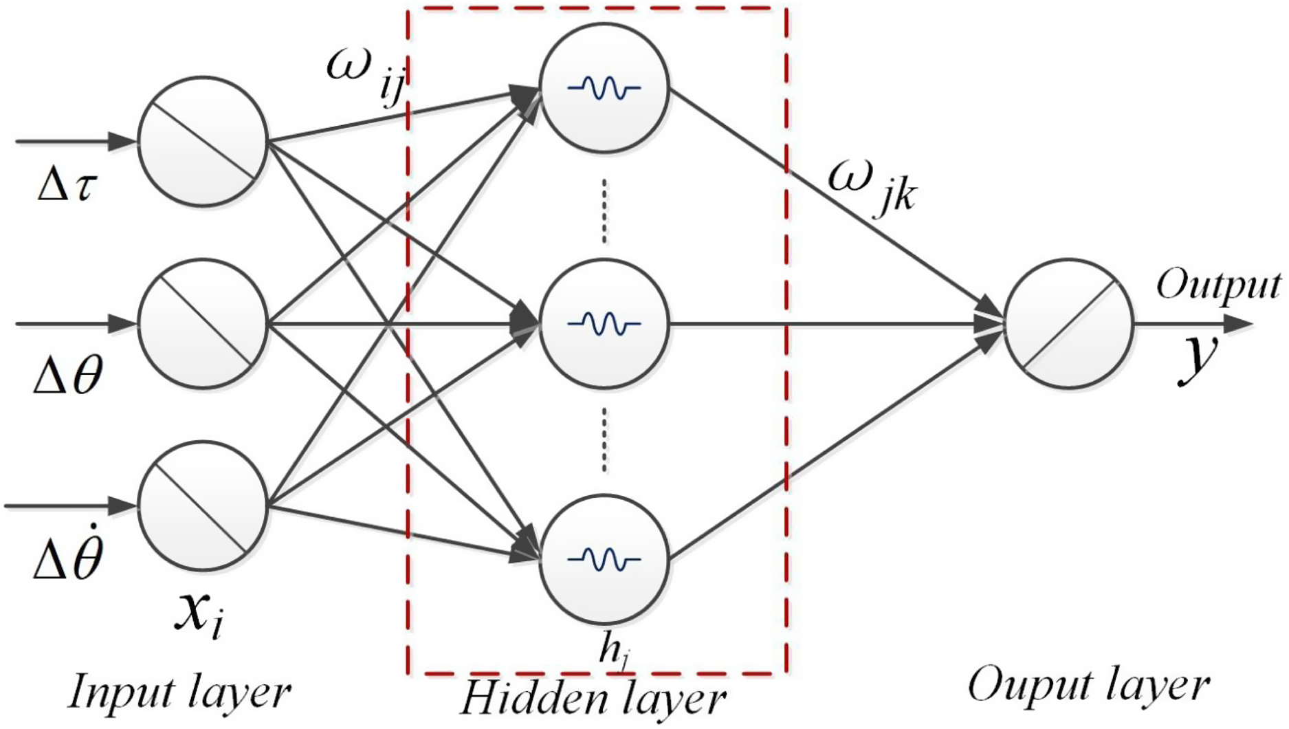
Figure 5. Structure diagram of RBF neural network.

The input layer of the RBF neural network is the vector x _i . When the inputs are different, the adjusted impedance parameters are also different. When the input is position error $\Delta{\theta}$ and force error $\Delta{\tau}$ , the output variable is the stiffness correction $\Delta$ K. The hidden layer of the RBF neural network is described as:

(13) \begin{equation} x_{j}=\sum _{i=1}^{m}\sum _{j=1}^{l}\omega _{ij}s_{j}=\sum _{j=1}^{l}\left(\omega _{1j}\Delta \tau +\omega _{2j}\Delta \dot{\theta }\right) \end{equation}

When the input is velocity error $\Delta \dot{\theta }$ and force error $\Delta{\tau}$ , the output variable is the damping correction $\Delta$ B.

(14) \begin{equation} x_{j}=\sum _{i=1}^{m}\sum _{j=1}^{l}\omega _{ij}s_{j}=\sum _{j=1}^{l}\left(\omega _{1j}\Delta \tau +\omega _{2j}\Delta \dot{\theta }\right) \end{equation}

(15) \begin{equation} d_{j}=f\!\left(x_{j}\right) \end{equation}

where m denotes the number of input variables; the RBF neural network designed in this paper has two input variables, that is, m = 2. s _j and d _j are the input and output of the hidden layer neural network nodes, respectively, and $\omega$ _ij is the weighting coefficient between the input layer and the hidden layer.

The activation function of the hidden layer neuron is:

(16) \begin{equation} f\!\left(x_{j}\right)=\exp\!\left(\!-\!\left\| x_{j}-c_{j}\right\| ^{2}/\left(2b_{j}^{2}\right)\right),j=1,2,\ldots,l \end{equation}

where c _j is the center of the basis function. b _j is the width of the basis function. l is the number of nodes in the hidden layer.

The output layer of the RBF neural network is described as:

(17) \begin{equation} y=\omega _{jk}d_{j}+f \end{equation}

(18) \begin{equation} y_{m}=\omega _{jk}d_{j} \end{equation}

where f is modeling error and external perturbation.y is the output value of the RBF network in the presence of the disturbance term f. y _m is the output value of the RBF network without f. $\omega$ _jk is the weighting coefficient between the hidden layer and the output layer.

The supervised learning method was used to train all parameters of the RBF neural network (center of RBF c _j , variance b _j, and weights between the hidden layer to the output layer $\omega$ _jk ). This is mainly done by performing gradient descent on the cost function and then correcting each parameters. Specifically, firstly, the parameters of RBF neural network are initialized randomly; then, the supervised training optimization is performed by gradient descent for all three parameters in the network. The cost function was set as:

(19) \begin{equation} E=\frac{1}{2}(y\mathit{-}y_{m})^{2} \end{equation}

Then in each iteration, the parameters are adjusted at a certain learning rate in the negative direction of the error gradient until the best parameter values are obtained.

(20) \begin{equation} c_{ij}\!\left(t\right)=c_{ij}\!\left(t-1\right)-\eta \frac{\partial E}{\partial c_{ij}\!\left(t-1\right)}+\alpha\!\left[c_{ij}\!\left(t-1\right)-c_{ij}\!\left(t-2\right)\right] \end{equation}

(21) \begin{equation} b_{ij}\!\left(t\right)=b_{ij}\!\left(t-1\right)-\eta \frac{\partial E}{\partial b_{ij}\!\left(t-1\right)}+\alpha \!\left[b_{ij}\!\left(t-1\right)-b_{ij}\!\left(t-2\right)\right] \end{equation}

(22) \begin{equation} \omega _{jk}\!\left(t\right)=\omega _{jk}\!\left(t-1\right)-\eta \frac{\partial E}{\partial \omega _{jk}\!\left(t-1\right)}+\alpha \!\left[\omega _{jk}\!\left(t-1\right)-\omega _{jk}\!\left(t-2\right)\right] \end{equation}

where c _ij (t) is the central component of the i _th hidden layer neuron for the j _th input neuron at the t times iteration; b _ij (t) is the width vector of the neuron corresponding to c _ij (t); $\omega$ _jk (t) is the conditioning weight between the j _th output neuron and the k _th hidden layer neuron at the t times iteration of computation. $\eta$ is learning rate, $\eta$ = 0.8. α is the momentum factor, α = 0.5.

3.4. Stability analysis

The Laypunov function was selected as:

(23) \begin{equation} V=X^{T}PX+\left\| \widetilde{{{\omega }}}_{jk}\right\| _{F}^{2} \end{equation}

There exists a positive definite matrix P, satisfying $A^{T}P+PA=-Q$ .

where Q is a given positive definite symmetric matrix.

(24) \begin{equation} \widetilde{{{\omega }}}_{jk}={\omega _{jk}}^{*}-\hat{\omega }_{jk} \end{equation}

where ${\omega _{jk}}^{*}$ is actual weight of RBF neural network, $\hat{\omega }_{jk}$ the estimated value of the weight.

Based on the theory of stability analysis of control systems, it is defined as:

(25) \begin{equation} \left\| \omega _{jk}\right\| _{\mathrm{F}}^{2}=tr\!\left({\widetilde{{{\omega }}}_{jk}}{}^{T}\widetilde{{{\omega }}}_{jk}\right)\geq 0 \end{equation}

where tr() is the trace of the matrix.

The modeling error and external perturbation f are described as:

(26) \begin{equation} f=\hat{\omega }_{jk}\varphi \!\left(x_{j}\right) \end{equation}

where $\phi$ (x _j ) is the output of the Gaussian basis function, and $\varphi (x_{j})=[f(x_{1}),f(x_{2}),\ldots f(x_{j}),\ldots f(x_{l})]$ .

The error state equation of the system is given by

(27) \begin{equation} \dot{X}=AX+B\left[f-\hat{f}\!\left(x,\omega _{jk}\right)\right] \end{equation}

where $X=\left[\begin{array}{l} e \\[5pt] \dot{e} \end{array}\right],A=\left[\begin{array}{l@{\quad}l} 0 & I\\[5pt] K_{p}& K_{d} \end{array}\right],B=\left[\begin{array}{l} 0\\[5pt] I \end{array}\right], \hat{f}$ is the estimated value of f.

The relevant term in Eq. (27) is transformed as:

(28) \begin{equation} f-\hat{f}\!\left(x,\omega _{jk}\right)=f-\hat{f}\!\left(x,{\omega _{jk}}^{*}\right)+f\!\left(x,{\omega _{jk}}^{*}\right)-\hat{f}\!\left(x,\omega _{jk}\right)=\beta +{\omega _{jk}}^{*T}\varphi \!\left(x_{j}\right)-{\hat{\omega }_{jk}}^{T}\varphi \!\left(x_{j}\right)=\beta +{\hat{\omega }_{jk}}^{T}\varphi \!\left(x_{j}\right) \end{equation}

where $\beta$ is the modeling error of the RBF neural network.

(29) \begin{equation} \dot{X}=AX+B\!\left(\beta +{\hat{\omega }_{jk}}{}^{T}\varphi \!\left(x_{j}\right)\right) \end{equation}

Then,

(30) \begin{equation} \dot{V}=X^{T}P\dot{X}+\dot{X}^{T}PX+2tr\!\left({\dot{\widetilde{{{\omega }}}}_{jk}}{}^{T}\widetilde{{{\omega }}}_{jk}\right)\enspace =\mathrm{X}^{T}P\!\left[AX+B\!\left(\beta +{\widetilde{{{\omega }}}_{jk}}{}^{T}\varphi \!\left(x_{j}\right)\right)\right]^{T}PX+2tr\!\left({\dot{\widetilde{{{\omega }}}}_{jk}}{}^{T}\widetilde{{{\omega }}}_{jk}\right) \end{equation}

Substitute Eq. (27) into Eq. (30) to obtain

(31) \begin{equation} \dot{V}=-X^{T}QX+\varphi ^{T}\!\left(x_{j}\right)\widetilde{{{\omega }}}_{jk}B^{T}PX+\beta ^{T}B^{T}PX+2tr\!\left({\dot{\widetilde{{{\omega }}}}_{jk}}^{T}\widetilde{{{\omega }}}_{jk}\right) \end{equation}

The adaptive rate is taken to be

(32) \begin{equation} \dot{\widetilde{{{\omega }}}}_{jk}=\varphi\!\left(x_{j}\right)X^{T}PB-k_{1}\left\| X\right\| \widetilde{{{\omega }}}_{jk} \end{equation}

where $k_{1}\left\| X\right\|$ is the robust term, k ₁ > 0, and satisfies $\left[B^{T}PX\varphi ^{T}\!\left(x_{j}\right)-k_{1}\left\| X\right\| \right]\widetilde{{{\omega }}}_{jk}+{\dot{\widetilde{{{\omega }}}}_{jk}}^{T}\widetilde{{{\omega }}}_{jk}=0$ .

Then,

(33) \begin{equation} \dot{V}=-X^{T}QX+2k_{1}\left\| X\right\| tr\!\left[\left({\dot{\widetilde{{{\omega }}}}_{jk}}^{T}\widetilde{{{\omega }}}_{jk}\right)\right]+2\beta ^{T}B^{T}PX \end{equation}

According to the parametric property, it is obtained that

(34) \begin{equation} tr\left({\dot{\widetilde{{{\omega }}}}_{jk}}^{T}\widetilde{{{\omega }}}_{jk}\right)\leq \left\| \widetilde{{{\omega }}}_{jk}\right\| _{F}\left\| \hat{\omega }_{jk}\right\| _{F}-\left\| \hat{\omega }_{jk}\right\| _{F}^{2} \end{equation}

Then,

(35) \begin{align} & \dot{V}\leq -X^{T}QX+2k_{1}\left\| X\right\| \left(\left\| \widetilde{{{\omega }}}_{jk}\right\| _{F}\left\| \hat{\omega }_{jk}\right\| _{F}-\left\| \hat{\omega }_{jk}\right\| _{F}^{2}\right)+2\beta ^{T}B^{T}PX\leq -\lambda _{\min }\!\left(Q\right)\left\| X\right\| ^{2} \nonumber \\[5pt] &\quad\;\; +k_{1}\left\| X\right\| \left(\left\| \widetilde{{{\omega }}}_{jk}\right\| _{F}\left\| \hat{\omega }_{jk}\right\| _{F}^{2}\right) +2\lambda _{\max }\!\left(P\right)\left\| \beta _{0}\right\| \left\| X\right\| \nonumber \\[5pt] & \quad\;\; =-\left\| X\right\| \left[\lambda _{\min }\!\left(Q\right)\left\| X\right\| +k_{1}\left[\left\| \widetilde{{{\omega }}}_{jk}\right\| _{F}-\frac{\left(\omega _{jk}\right)_{\max }}{2}\right]^{2}-\frac{k_{1}}{4}\left(\omega _{jk}\right)^{{2}}_{\max }-\left\| \beta _{0}\right\| \lambda _{\max }\!\left(P\right)\right] \end{align}

where λ _min (Q) is the minimum eigenvalue of matrix Q and λ _max (P) is the maximum eigenvalue of matrix P.

For $\dot{V}\leq 0$ , the following conditions need to be satisfied.

(36) \begin{equation} \lambda _{\min }\!\left(Q\right)\!\left\| X\right\| \geq \frac{k_{1}}{4}\!\left(\omega _{jk}\right)^{{2}}_{\max }+\left\| \beta _{0}\right\| \lambda _{\max }\!\left(P\right) \end{equation}

4.1. Parameters setting

A human model with 170 cm height and 70 kg weight was set as the study subject, whose thigh length was about 380 mm, calf-length approximately 400 mm, and ankle height about 80 mm. The motion simulation process is shown in Fig. 6. The input of joint trajectories was obtained by human gait experiments. A healthy subject with the age of 25, the weight of 70 kg, and the height of 170 cm is recruited for the experiment, just as shown in Fig. 7. Before the gait experiment, all subjects were given a detailed explanation of the test content and signed a consent form for voluntary participation in the experiment. The subjects had no surgery, no history of lower extremity trauma, no balance problems, or neural muscular disorders within the past six months. A written consent is obtained from the subject. The test environment was a linear walkway of 5 m in length and 1 m in width. The kinematic parameters were acquired by VICON acquisition system(Oxford Metrics Ltd, Oxford, UK). The data acquisition frequency is 1200 Hz.

Figure 6. Simulation process of human-machine coupling model.

Figure 7. Gait experiment diagram.

To verify the effectiveness and superiority of the proposed method, the simulation results are compared with those of torque feedback controller [Reference Zhang, Cheah and Collins32], impedance controller [Reference Li, Liu, Yan, Zhang, Li and Zhang33], and FVI controller [Reference Zhang, Wu, Chen, Wu and Liu34]. And the parameters of each control method are set, as shown in Table II. The excellent agreement between the reference trajectory and the actual trajectory illustrates the effectiveness of the measurement and control methods.

Table II. The parameters of each controller.

The RBF neural network includes three layers. The input layer contains two nodes with hip error function and knee error function; the hidden layer uses Gaussian basis function as the excitation function, the center vector is [−2 −1 0 1 2], and the width is 0.5; the adaptive rate is taken as 30. The root mean square accuracy was set to 0.01 as the termination condition of the RBF neural network. The moment coefficient of 0.8 is selected, and the simulation is performed at a speed of 0.2 m/s.

4.2. Simulation results analysis

The joint trajectory tracking results of each controller and trajectory error results are shown in Figs. 8, 9, 10 and 11, respectively. When the traditional torque feedback control method was used to perform the motion mission, the maximum error values of the hip joint and knee joint between the exoskeleton robot and the human were 7.8 and 15.1 deg, respectively. Due to the large weight-bearing ratio of the limb, the release of human muscle force has more excellent resistance, so the tracking performance of the human joint position to the exoskeleton robot joint position is poor, and the two have a significant error. The angle deviation needs to be reduced by impedance relationship adjustment. Compared with the torque feedback control system without the impedance control adjustment module, the exoskeleton robot obtained by impedance control has a smaller range of error in the joint angle with the human model. The maximum error of the exoskeleton robot and human hip joint angle is 4.3 deg. This indicates that the exoskeleton robot control system converts the interaction force difference into angular deviation according to the change of human-machine contact force and adjusts the input torque in real-time. The exoskeleton robot provides greater torque support during the limb muscle strength deficiency phase and improves human tracking performance. The maximum angle error values of the hip joint and knee joint obtained based on the fuzzy impedance control method were 3.2 and 9.2 deg, respectively. The error range of the joint angle between the exoskeleton robot and human model is smaller, indicating that the impedance controller with real-time adjustment of impedance parameters improves the control system’s control accuracy and the human-machine coupling suppleness better. After adding the neural network error compensation function module, the maximum angle error values of the hip joint and knee joint were reduced to 2.4 and 2.2 deg, respectively. This indicates that the neural network compensation has a good suppression effect on the uncertainty term of the system.

Figure 8. Hip trajectory tracking results of each controllers.

Figure 9. Trajectory error results of hip joint.

Figure 10. Knee trajectory tracking results of each controllers.

Figure 11. Trajectory error results of knee joint.

5.1. Experimental platform

Human-machine coupling experiments are conducted to demonstrate the functionality of the proposed control method. The exoskeleton robot platform is shown in Fig. 12. The joint motion range of the exoskeleton is 20° flexion and 40° extension for the hip joint, and 70° flexion and 0° extension for the knee joints, and 0° plantarflexion and 20° dorsiflex for ankle joints. The control system consists of the data processor Raspberry Pi and the motion controller STM32F103. Raspberry Pi is used to process data collected from angle sensors (AD36/1217AF. ORBVB, Hengstler, Germany) and torque sensors(TRX-50N·m, Italy). The communication mode between the data processor and motion controller is parallel port communication. The motion controller controls the motors through the controller area network Fieldbus. A healthy subject with the age of 25, the weight of 68 kg, and the height of 170 cm is recruited for the experiment. A written consent is obtained from the subject. For safety reasons, if the angle of the exoskeleton is greater than the allowable value, the exoskeleton will be forced to stop moving by software. In addition, the subjects could cut off the power through the emergency switch button. We intercepted the complete gait course of the left lower limb during the swing phase. The video capture of the human experiment is shown in Fig. 13. The time of a complete gait cycle is 3.5 s. The experiment demonstrates that the exoskeleton robot can effectively assist the human body to realize stable walking.

Figure 12. The exoskeleton robot platform.

Figure 13. Video screenshots of the human experiment.

5.2. Human-machine system testing

A current safety threshold is set to ensure the safety of the contact force between the exoskeleton and the subject. When the human-machine contact force makes the current within the threshold value, the movement of the joint does not stop. When the contact force exceeds the current threshold, the joint stops moving. When the human-machine contact force becomes larger, the joint torque of the exoskeleton will be correspondingly larger to resist the obstructive force exerted by the human body, and the current output will become larger at this time. The system simultaneously detects whether the current of each joint exceeds the threshold. According to the relationship between torque and power of servo motor,

(37) \begin{equation} \tau _{m}=\frac{9550P}{n} \end{equation}

where P is the power of motor, P = UI, U is voltage of motor, I is current of motor. n is rational speed of motor. The current is proportional to the torque. The excessive torque output may cause secondary injury to the wearer. Generally, the torque required for joint movement does not exceed 200 N.m. According to the ammeter test, when the torque value reaches 200 N.m, the current value is about 4A. Hence, the current safety threshold was set as 4A.

We conducted experiments on the exoskeleton under conditions of unloaded(red line) and loaded(black line). The real-time current value of hip joint and knee joint are shown in Figs. 14 and 15, respectively. When the exoskeleton is in continuous contact with the subject, the current value will increase with the contact force (resistance torque) compared to the unstressed condition. We found that the current was not exceeded the current safety threshold during the entire gait cycle, indicating that the coupling performance of the human-machine system was good. To test the system’s safety, we let the subject deliberately increase the range of hip joint motion to increase the human-machine contact force. Then, the joint will stop at the point S when the current generated by the contacted force exceeds the threshold value, just as shown in Fig. 15. The test ensures the safety of the exoskeleton system.

Figure 14. Real-time currents in hip joint when in stressed and unstressed conditions.

Figure 15. Real-time currents in knee joint when in stressed and unstressed conditions.

We analyzed the variation of the human joint torque, exoskeleton joint torque, and human-machine interaction torque, respectively, and the experimental results are shown in Figs. 16 and 17. It can be seen that the torque output curves of the exoskeleton and the human remain the same trend under the action of the proposed controller in this study. And the human torque always remains at a lower torque output, which is due to the exoskeleton robot compensating the required torque of the human body. It is worth noting that at 1.5 s, the human knee joint torque increases suddenly, and the exoskeleton joint torque decreases sharply, which is because the exoskeleton robot’s motion control has a specific time delay behavior at the moment of phase transition and fails to make the symbolic human intention action in time. At this time, the human-machine interaction torque also increases accordingly. We found that this situation cannot be avoided after several experiments, which is the critical problem we will solve next. The overall tendency is smooth in term of the human-machine interaction torque, and the average values of interaction torque of hip joint and knee joint are 3.215 and 2.374 N.m, indicating that the control algorithm proposed in this study can achieve stable and smooth walking.

Figure 16. Torque value of hip joint.

Figure 17. Torque value of knee joint.