


1. Introduction
The statistical properties of ocean surface waves and associated quantities such as wave heights and crest heights is a much studied topic with widespread engineering applications. It is well known that to leading order, a random sea surface can be described as a Gaussian random field, while in higher-order approximations, non-Gaussian effects arise due to the nonlinearity of the waves.
The description of nonlinear random waves was first considered by Tick (Reference Tick1959), Hasselmann (Reference Hasselmann1962) and Longuet-Higgins (Reference Longuet-Higgins1963), who, based on perturbation expansions of the governing nonlinear equations, derived expressions for the second-order nonlinear surface elevation. This is often referred to as second-order random wave theory (see also Sharma & Dean Reference Sharma and Dean1979), and provides the expressions for the bound harmonics arising from non-resonant nonlinear interactions up to second order. The extension of second-order theory to include higher-order bound waves up to fourth order was derived within the framework of the Hamiltonian theory of water waves (Zakharov Reference Zakharov1968) by Krasitskii (Reference Krasitskii1994) in terms of the canonical transformation that eliminates bound waves (non-resonant interactions) from the Zakharov equation, and hence expresses all bound waves in terms of the free waves.
The statistical properties of the second-order random sea surface were first studied by Longuet-Higgins (Reference Longuet-Higgins1963), who showed that the probability density function of the surface elevation can be expressed as a Gram–Charlier/Edgeworth-type expansion. The corresponding Gram–Charlier/Edgeworth-based distributions of e.g. wave envelopes and wave heights were considered first by Bitner (Reference Bitner1980). Since then, numerous related approaches and methods have been applied to approximate the statistical distributions of weakly nonlinear random waves (see e.g. Ochi Reference Ochi1998; Machado Reference Machado2003; Tayfun & Alkhalidi Reference Tayfun and Alkhalidi2020, for a detailed overview). Common for most such methods is that the deviation from Gaussianity is represented through non-zero higher-order cumulants of the surface elevation distribution, often expressed in terms of non-zero skewness and excess kurtosis. Thus the skewness and kurtosis of the ocean surface are important parameters that appear in various theoretically based distributions for surface elevation, wave heights and crest heights (see e.g. Tayfun Reference Tayfun2006; Tayfun & Fedele Reference Tayfun and Fedele2007; Tayfun & Alkhalidi Reference Tayfun and Alkhalidi2020, and references therein). Hence knowledge of the skewness and kurtosis of a random wave field provides also information about the associated statistical distributions.
An expression for the skewness of a second-order random wave field in deep water was derived by Longuet-Higgins (Reference Longuet-Higgins1963). Later, general expressions for the sea surface skewness and kurtosis in a random directional wave field in finite water depth, including effects up to third order, were derived by Janssen (Reference Janssen2009) starting from Krasitskii's canonical transformation (Krasitskii Reference Krasitskii1994). Although the general integral expressions for skewness and kurtosis for any given wave field are given in Janssen (Reference Janssen2009), the direct evaluation of these integrals has not been considered widely, and most existing applications discussing distributions of e.g. wave heights or crest heights rely on various approximations and simplifications (e.g. Vinje Reference Vinje1989; Winterstein, Bitner-Gregersen & Ronold Reference Winterstein, Bitner-Gregersen and Ronold1991; Vinje & Haver Reference Vinje and Haver1994; Winterstein & Jha Reference Winterstein and Jha1995; Jha & Winterstein Reference Jha and Winterstein2000; Tayfun Reference Tayfun2006). To our knowledge, the only existing work addressing the exact evaluation of the integral expressions for both skewness and kurtosis is by Annenkov & Shrira (Reference Annenkov and Shrira2014), who used a numerical approach similar to that suggested in the present paper to calculate the skewness and kurtosis for various JONSWAP spectra in infinite water depth.
The main objective of the present work is to develop a numerically efficient method for solving the integral expressions for surface elevation skewness and kurtosis, and to use this method to propose new, accurate parametrizations for skewness and kurtosis as functions of sea-state parameters. These new parametrizations can then be used in higher-order distributions for surface elevation, crest heights and wave heights, where skewness and kurtosis appear as distribution parameters. The paper is organized as follows. First, some relevant background, including a review of existing parametrization of skewness and kurtosis, is given in § 2. The numerical method for solving the exact integrals for skewness and kurtosis, including validation of the numerical approach, is presented in § 3. Then in § 4, the numerical method is applied to calculate the exact skewness and kurtosis for a large number of different wave spectra, covering the range of realistic sea-state conditions encountered in ocean regions of deep and intermediate water depths. This is then used to evaluate the accuracy of existing parametrizations of skewness and kurtosis, and to propose new, more accurate parametrizations of skewness and kurtosis as functions of sea-state steepness, water depth, spectral bandwidth and directional spreading. Some comparisons with model-test results and phase-resolved simulations are presented in § 5. Finally, some discussion and examples of using the exact skewness and kurtosis in higher-order crest height distributions are given in § 6.
2. Background
The skewness  $\lambda _3$ and excess kurtosis
  $\lambda _4$ of a random variable
  $X$ are defined by
 \begin{equation} \lambda_3={E}\left[\left({\frac{X-\mu}{\sigma}}\right)^{3}\right]=\frac{\mu_{3}}{\sigma^{3}}=\frac{\kappa_{3}}{\kappa_{2}^{3/2}} \end{equation}
and
 \begin{equation} \lambda_4={E}\left[\left({\frac{X-\mu}{\sigma}}\right)^{4}\right]-3=\frac{\mu_{4}}{\sigma^{4}}-3=\frac{\kappa_4}{\kappa_2^2}. \end{equation}
Here,  ${E}[\,{\cdot}\, ]$ denotes the statistical expectation,
  $\mu ={E}[X]$ is the mean,
  $\sigma ^2=\mu _2={E}[(X-\mu )^{2}]$ is the variance,
  $\mu _j={E}[(X-\mu )^{j}]$ is the
  $j$th central moment, and
  $\kappa _2=\mu _2=\sigma ^2$,
  $\kappa _3=\mu _3$ and
  $\kappa _4=\mu _4-3\mu _2^2$ are the cumulants. For a Gaussian distribution, all cumulants above second order vanish, so both skewness and excess kurtosis are zero.
Starting from Krasitskii's canonical transformation, the general expressions for the sea surface skewness and kurtosis in a random directional wave field in finite water depth, including non-resonant nonlinear interactions up to third order, were derived by Janssen (Reference Janssen2009) in terms of integrals involving the leading-order (free-wave) wave-vector spectrum  $E(\boldsymbol {k})$, in the forms
 \begin{equation} \lambda_3=\frac{3}{m_0^{3/2}}\int E_1E_2K_{1,2}^{(3)}\,\textrm{d}\boldsymbol{k}_{1,2},\quad \lambda_4=\frac{12}{m_0^2}\int E_1E_2E_3K_{1,2,3}^{(4)}\,\textrm{d}\boldsymbol{k}_{1,2,3}, \end{equation}
where
 $$\begin{gather} K_{1,2}^{(3)}=\mathscr{A}_{1,2}+\mathscr{B}_{1,2}, \end{gather}$$
 $$\begin{gather}K_{1,2,3}^{(3)}=(\mathscr{A}_{1,3}+\mathscr{B}_{1,3})(\mathscr{A}_{2,3}+\mathscr{B}_{2,3})+\tfrac{1}{2}\mathscr{D}_{1+2+3,1,2,3}+\tfrac{1}{2}\mathscr{C}_{1+2-3,1,2,3}. \end{gather}$$
Here,  $m_0=\int E(\boldsymbol {k})\,\textrm {d}\boldsymbol {k}$ is the zeroth spectral moment, and a compact subscript notation is used for functional dependence of wavenumbers, i.e.
  $E_1=E(\boldsymbol {k}_1)$,
  $\mathscr {D}_{1+2+3,1,2,3}=\mathscr {D}(\boldsymbol {k}_1+\boldsymbol {k}_2+\boldsymbol {k}_3,\boldsymbol {k}_1,\boldsymbol {k}_2,\boldsymbol {k}_3)$,
  $\textrm {d}\boldsymbol {k}_{1,2}=\textrm {d}\boldsymbol {k}_1\,\textrm {d}\boldsymbol {k}_2$, and so on. The functions
  $\mathscr {A}$,
  $\mathscr {B}$,
  $\mathscr {C}$ and
  $\mathscr {D}$ are expressed in terms of the kernel functions in the canonical transformation of Krasitskii (Reference Krasitskii1994) and can be found in Janssen (Reference Janssen2009).
It should be noted that when considering nonlinearities beyond second order, there are, in addition to the bound waves represented by the canonical transformation (i.e. non-resonant interactions), also non-Gaussian effects due to resonant and near-resonant interactions (i.e. free-wave modulations). These effects are described in terms of evolution equations for the free waves as described by e.g. the Zakharov equation (Zakharov Reference Zakharov1968), and in the statistical theory by the Hasselmann kinetic equation (Hasselmann Reference Hasselmann1962). To third order, there is a contribution to the kurtosis from free-wave modulations, which has been studied in e.g. Janssen (Reference Janssen2003), Mori & Janssen (Reference Mori and Janssen2006) and Janssen & Janssen (Reference Janssen and Janssen2019). The dynamic contribution to the kurtosis is time-dependent and hence not easily incorporated in a stationary description of random sea states, which is the focus here. This contribution is therefore not considered in this paper. It is, however, known that for realistic, directionally spread ocean wave spectra, the effect of the dynamical kurtosis is small (Annenkov & Shrira Reference Annenkov and Shrira2014) and decays to zero asymptotically in the long-time limit, i.e. on the time scale of the Hasselmann equation (Janssen & Janssen Reference Janssen and Janssen2019).
2.1. Existing parametrizations of skewness and kurtosis
In the following, some parametrizations of skewness and kurtosis that have been presented in existing works are reviewed. These existing parametrizations are derived under various simplifying assumptions with respect to e.g. directionality, water depth and type of spectral shape. A schematic overview of the different existing works is presented in table 1, while more details are given in §§ 2.1.1–2.1.5.
Table 1. Summary of existing parametrizations of skewness and kurtosis, with respect to the main assumptions made in the analyses. The first column (‘Order’) indicates the nonlinear order to which the analyses are valid. The second and third columns indicate whether parametrizations for skewness ( $\lambda _3$) and kurtosis (
 $\lambda _4$) were considered. The fourth column (‘Spectrum’) indicates the type of spectrum considered. The fifth column (
 $h$) shows the water-depth regimes considered. The final column shows whether unidirectional/one horizontal dimension (1-D) or directional/two horizontal dimensions (2-D) waves were considered.

2.1.1. Narrow-band limits
Narrow-band expressions for the skewness and kurtosis were first presented for deep-water waves including second-order effects by Tayfun (Reference Tayfun1980), and more generally for finite water depth including up to third-order effects by Janssen (Reference Janssen2009). Formally, the narrow-band limits can be obtained by assuming  $E(\boldsymbol {k})=m_0\delta (\boldsymbol {k}-\boldsymbol {k}_c)$ in (2.3a,b), where
  $\boldsymbol {k}_c=(k_p,0)$, and
  $\delta$ is the Dirac delta function. As shown by Janssen (Reference Janssen2009), the narrow-band limits of (2.3a,b) are
 \begin{equation} \lambda_3=6\epsilon(\alpha+\varDelta),\quad \lambda_4=24\epsilon^2 \big(\beta + \gamma + 2(\alpha + \varDelta)^2\big), \end{equation}
where
 \begin{align} \alpha=\frac{3-\tau^2}{4\tau^3},\ \ \ \beta=\frac{3}{64\tau^6}\big[8 + (1 - \tau^2)^3\big],\ \ \ \gamma=-\frac{\alpha}{2},\ \ \ \tau=\tanh(k_ph), \ \ \ \epsilon=k_p\sqrt{m_0}. \end{align}
The coefficient  $\varDelta$ arises from the wave-induced mean level – see the discussion in Janssen (Reference Janssen2009). The correct form of
  $\varDelta$ is, however, still associated with some uncertainty due to the fact that it arises from a non-unique limit in the kernel function of the Zakharov equation (Janssen & Onorato Reference Janssen and Onorato2007; Janssen Reference Janssen2009; Stiassnie & Gramstad Reference Stiassnie and Gramstad2009; Gramstad Reference Gramstad2014; Pezzutto & Shrira Reference Pezzutto and Shrira2023). In a purely unidirectional setting, the limit could be found uniquely, in which case
  $\varDelta$ takes the form
 \begin{equation} \varDelta_{1D}=-\frac{1}{1-\rho^2}\left(\frac{1-\tau^2}{2\tau}+\frac{1}{4k_ph}\right), \end{equation}
which is in agreement with the unidirectional analysis of Whitham (Reference Whitham1974). Here,
 \begin{equation} \rho=\frac{c_g}{c_s}=\sqrt{\tau k_ph}\left(\frac{1 - \tau^2}{2\tau} + \frac{1}{2k_ph}\right) \end{equation}
is the group velocity  $c_g$ normalized by the shallow-water wave velocity
  $c_s=\sqrt {gh}$.
For waves in two horizontal dimensions, the non-unique limit depends on the direction from which the limit is approached. In Janssen (Reference Janssen2009), it was suggested to use the one-dimensional result also for directional waves, leading to  $\varDelta$ in the form (2.7). Later, in Janssen (Reference Janssen2017), a modified form of
  $\varDelta$ was suggested in which finite bandwidth effects are accounted for. However, this form involves parameters describing the spectral bandwidths in frequency and direction, and the actual value of
  $\varDelta$ will depend on how these spectral bandwidths are defined, a discussion that is outside the scope of the present paper.
Recently, a proposed resolution of the non-uniqueness problem was suggested by Pezzutto & Shrira (Reference Pezzutto and Shrira2023), leading to a modification of (2.7) in the form
 \begin{equation} \varDelta_{PS}=-\frac{1}{1-\rho^2}\left(\frac{(J_0+J_2)(1-\tau^2)}{4\tau}+\frac{J_2}{4k_ph}\right), \end{equation}
where
 \begin{equation} J_0=\sqrt{1-\rho^2},\quad J_2=\frac{\sqrt{1-\rho^2} - 1 + \rho^2}{\rho^2}. \end{equation}
Note that setting  $J_0=J_2=1$ gives the unidirectional result (2.7).
An important point to note is that the choice of the limit leading to  $\varDelta$ (see the last equation on p. 39 in Janssen Reference Janssen2009) is relevant not only for the narrow-band expressions, but also for the numerical evaluation of the general integral expressions (2.3a,b). This is because the non-unique limit is encountered in the kernel functions of these integrals, and in the numerical evaluation of the integrand, these limits should be chosen according to the discussion above. Following Janssen (Reference Janssen2009) and Pezzutto & Shrira (Reference Pezzutto and Shrira2023), for purely unidirectional waves we choose the limits so that
  $\varDelta =\varDelta _{1D}$, and for directional waves we have for completeness considered both
  $\varDelta =\varDelta _{PS}$ and
  $\varDelta =\varDelta _{1D}$. Interestingly, the difference between choosing
  $\varDelta =\varDelta _{PS}$ and
  $\varDelta =\varDelta _{1D}$ for directional wave fields turns out to be minor for a finite bandwidth spectrum (it was found to be less than 1 % in the more than 18 000 spectra considered in this study), despite the fact that the effect of the choice of
  $\varDelta$ on the narrow-band result can be quite significant in shallow-water depth. This is illustrated in figure 1, which shows the skewness and kurtosis according to the narrow-band limits when using either
  $\varDelta _{1D}$ or
  $\varDelta _{PS}$. This is compared to results from exact integration of (2.3a,b) for a spectrum with very narrow directional distribution, as well as for a purely one-dimensional spectrum. As seen from the figure, for a one-dimensional spectrum, the exact results are in good agreement with the narrow-band approximation with
  $\varDelta =\varDelta _{1D}$. However, when adding a small directional distribution to the spectrum, the exact results deviate from both versions of the narrow-band approximation, but show virtually no effect of whether
  $\varDelta _{1D}$ or
  $\varDelta _{PS}$ were used as the limit of the non-unique terms in the integrand.

Figure 1. (a) Skewness  $\lambda _3$ and (b) kurtosis
  $\lambda _4$ according to narrow-band expressions (solid lines), exact integration of a two-dimensional spectrum with narrow directional spreading (dashed lines), and a purely one-dimensional spectrum (dotted lines). Blue lines show results obtained using
  $\varDelta =\varDelta _{1D}$, while orange lines show results for
  $\varDelta =\varDelta _{PS}$. The spectrum that was used here is a JONSWAP spectrum with
  $\gamma =10.0$,
  $\epsilon =0.1$ and
  $\sigma _{\theta }=2.5^\circ$ (see § 4 for details).
In deep water,  $\varDelta =0$, and the expressions for skewness and kurtosis take the simple forms
  $\lambda _3=3\epsilon$ and
  $\lambda _4=18\epsilon ^2$. For historical reasons, it should be mentioned that different expressions for the deep-water limit of the narrow-band skewness and kurtosis are reported in the literature. It turns out that these differences can be traced down to different assumptions in the derivations regarding the representation of the underlying Stokes wave expansion, as summarized in table 2. Here, it is noted that taking the narrow-band limit corresponds to a Stokes wave with first-order amplitude
  $a=\sqrt {2m_0}$ and wavenumber
  $k_p$, and below we use
  $\epsilon _s=ak_p$ to denote the steepness parameter for the Stokes wave, to distinguish it from the sea-state steepness
  $\epsilon =k_p\sqrt {m_0}$.
Table 2. Narrow-band deep-water expressions for skewness and kurtosis reported in the literature, and their corresponding Stokes wave expansions.

 $^{a}$The second-order model is not sufficient to evaluate kurtosis to
  $O(\epsilon ^2)$ since there are contributions to
  $O(\epsilon ^2)$ also from third order.
 $^{b}$This expression is not given explicitly in Winterstein et al. (Reference Winterstein, Bitner-Gregersen and Ronold1991) but can be deduced easily by combining their (27) and (29).
It has been verified that all expressions for skewness and kurtosis reproduced in table 2 can be obtained by ‘randomizing’ the corresponding Stokes wave, i.e. by assuming that  $a$ is Rayleigh distributed with parameter
  $\sigma$, and that
  $\theta$ is distributed uniformly on
  $[0, 2{\rm \pi} )$. Apart from the fact that Tayfun (Reference Tayfun1980) did not consider third-order terms, there are two main sources of differences between the results in table 2: the constant second-order term
  $\epsilon _s/2$ appearing in Vinje (Reference Vinje1989) and Winterstein et al. (Reference Winterstein, Bitner-Gregersen and Ronold1991), and the third-order correction to the
  $\cos {\theta }$ term appearing in Vinje (Reference Vinje1989), Mori & Janssen (Reference Mori and Janssen2006) and Janssen (Reference Janssen2009). The constant second-order term corresponds to a change in the mean water level and is discussed in Tayfun (Reference Tayfun1986), where it is argued that this term should not be included. The third-order correction to the
  $\cos {\theta }$ term arises naturally when starting from the canonical transformation of Krasitskii (Reference Krasitskii1994), and is discussed further in Janssen (Reference Janssen2009). The reasons for the coefficients of this term reported in Vinje (Reference Vinje1989) and Mori & Janssen (Reference Mori and Janssen2006) are not clear, and may be due to errors/misprints.
2.1.2. Vinje & Haver (Reference Vinje and Haver1994)
Using a second-order stochastic model, Vinje & Haver (Reference Vinje and Haver1994) suggested the following approximations for skewness and kurtosis:
 \begin{equation} \lambda_3=\frac{34.4H_s}{gT_p^2}+2.14\times 10^{-6}\left(\frac{gT_p^2}{h}\right)^3,\quad \lambda_4=3\lambda_3^2. \end{equation}
The first term in the expression for the skewness was derived theoretically for a unidirectional Pierson–Moskowitz spectrum (corresponding to JONSWAP with  $\gamma =1$), while the second term is a finite-depth correction based on field measurements.
2.1.3. Winterstein & Jha (Reference Winterstein and Jha1995), Jha & Winterstein (Reference Jha and Winterstein2000)
Using a second-order random model, Winterstein & Jha (Reference Winterstein and Jha1995) estimated skewness and kurtosis for a wide range of different unidirectional JONSWAP sea states in different water depths. They fitted the following expressions for skewness and kurtosis, as functions of wave steepness, JONSWAP peakedness factor  $\gamma$ and water depth
  $h$:
$h$:
 \begin{equation} \lambda_3=\left(5.45\gamma^{-0.084} + 0.135\left(h/L_p\right)^{-1.22}\right)S_p,\quad \lambda_4=1.41\gamma^{-0.02}\lambda_3^2, \end{equation}
where  $L_p=gT_p^2/(2{\rm \pi} )$ is the characteristic wavelength obtained from
  $T_p$ through the linear deep-water dispersion relation, and
  $S_p=H_s/L_p=2{\rm \pi} H_s/(gT_p^2)$ is a measure for the sea-state steepness.
In a later paper (Jha & Winterstein Reference Jha and Winterstein2000), a slightly different fit for the skewness was reported in the form
 \begin{equation} \lambda_3=\left(5.45\gamma^{-0.084} + \left[\exp{\left(7.41\left(h/L_p\right)^{1.22}\right)} - 1\right]^{-1}\right)S_p. \end{equation}
2.1.4. Tayfun–Forristall
In Tayfun (Reference Tayfun2006), a representation for the skewness was obtained by relating the theoretical Gram–Charlier-based second-order crest distribution to Forristall's Weibull fit to second-order crest heights (Forristall Reference Forristall2000). By matching the moments of the theoretical distribution of crest heights to the Forristall distribution, Tayfun (Reference Tayfun2006) derived the following expression for the skewness:
 \begin{equation} \lambda_3=48\,\frac{\alpha^3}{\beta}\,\varGamma\left(\frac{3}{\beta}\right)-\frac{3}{4}\sqrt{\frac{\rm \pi}{2}}, \end{equation}
where  $\alpha$ and
  $\beta$ are the parameters in the Forristall distribution, for which parametrizations in terms of water depth and sea-state steepness are given in Forristall (Reference Forristall2000).
2.1.5. Annenkov & Shrira (Reference Annenkov and Shrira2014)
Annenkov & Shrira (Reference Annenkov and Shrira2014) solved the exact integrals for the skewness and kurtosis (2.3a,b) for different types of JONSWAP spectra in infinite water depth. Based on their results, they suggested the following fit for the kurtosis:
 \begin{equation} \lambda_4=25.2\gamma^{-0.328}\epsilon^2. \end{equation}
A fit for the skewness was also reported in Annenkov & Shrira (Reference Annenkov and Shrira2014), but due to an error in their computations, this is not correct (Victor Shrira, personal communication), and therefore is not considered here. Note that, different from Winterstein & Jha (Reference Winterstein and Jha1995) and Jha & Winterstein (Reference Jha and Winterstein2000), the results of Annenkov & Shrira (Reference Annenkov and Shrira2014) include third-order effects needed for a consistent calculation of kurtosis to  $O(\epsilon ^2)$. However, (2.15) also includes an estimate for the dynamical part of the kurtosis, and is therefore not directly comparable to the other parametrizations considered above, or to the results presented in this paper. The dynamical kurtosis is, however, relatively small for realistic directional spectra, typically within
  ${\pm }15\,\%$ of the bound kurtosis for the spectra considered in Annenkov & Shrira (Reference Annenkov and Shrira2014).
3. Numerical method and convergence tests
A numerical method for solving the exact integral expressions for the skewness and kurtosis, (2.3a,b), has been developed and tested, as described in the following.
It was found to be convenient to employ a change of variables from  $\boldsymbol {k}=(k_x, k_y)=(k\cos {\theta }, k\sin {\theta })$ to
  $(\omega, \theta )$. Using that
  $E(\boldsymbol {k})=S(\omega,\theta ){c_g}/{k}$ and
  $\textrm {d} k_x\,\textrm {d} k_y=({k}/{c_g})\,\textrm {d}\omega \,\textrm {d}\theta$, where
  $k=|\boldsymbol {k}|$,
  $c_g=\textrm {d}\omega /\textrm {d} k$ and
  $\omega ^2=gk\tanh {(kh)}$, one can write
 \begin{equation} \lambda_3=\frac{3}{m_0^{3/2}}\int S_1S_2K_{1,2}^{(3)}\,\textrm{d}\omega_{1,2}\,\textrm{d}\theta_{1,2},\quad \lambda_4=\frac{12}{m_0^2}\int S_1S_2S_3K_{1,2,3}^{(4)}\,\textrm{d}\omega_{1,2,3}\,\textrm{d}\theta_{1,2,3}. \end{equation}
The integrals were then approximated numerically using a discretization of the integration space. For  $\omega$, a logarithmically spaced grid from
  $\omega _{min}$ to
  $\omega _{max}$ was used, while for
  $\theta$, a regular discretization on the interval from
  $\theta _{min}=-{\rm \pi} /2$ to
  $\theta _{max}={\rm \pi} /2$ was employed. The number of grid points and the integration limits were chosen based on the convergence tests described in the following. For future applications to spectra having energy also in directions
  $|\theta |>{\rm \pi} /2$, the integration space with respect to
  $\theta$ would need to be extended.
The convergence tests presented below were all carried out using a JONSWAP spectrum with sea-state steepness  $\epsilon =k_p\sqrt {m_0}=0.1$ and peakedness factor
  $\gamma =3.3$ for a water depth corresponding to non-dimensional depth
  $k_ph=1.0$. A directional distribution of the type
  $\cos ^n{(\theta )}$ with
  $n=7$ was used, corresponding to a directional spreading
  $\sigma _{\theta }\approx 20^\circ$ (see (4.1a,b) and (4.2) for definitions of the spectral shape and the directional spreading parameter
  $\sigma _{\theta }$). Some additional convergence tests were carried out also for different spectral shapes (i.e. different values for
  $\gamma$ and
  $n$), with similar results.
The convergence of the results with respect to the maximum frequency  $\omega _{max}$ of the integration domain is shown in figure 2(a). The error is calculated relative to the results obtained when using
  $\omega _{max}=30\omega _p$. Based on these results, it was decided to use
  $\omega _{max}=5\omega _p$, yielding an error less than 1 %. Here,
  $\omega _p$ is the peak frequency of the JONSWAP spectrum.

Figure 2. (a) Convergence of calculated skewness and kurtosis with respect to size of integration domain  $\omega _{max}$. (b) Computational time (using parallel implementation on 64 cores) for calculation of skewness and kurtosis as functions of number of points used to discretize integral in each dimension. (c) Error in calculated skewness as function of
  $n_{\omega }$ for different values of
  $n_{\theta }$. (d) Error in calculated kurtosis as function of
  $n_{\omega }$ for different values of
  $n_{\theta }$.
The accuracy of the calculated values of skewness and kurtosis with respect to the number of points used to discretize the integration domain  $\omega \in [0.5\omega _p, 5\omega _p]$ and
  $\theta \in [-{\rm \pi} /2, {\rm \pi}/2]$ are shown for skewness and kurtosis in figures 2(c) and 2(d), respectively. Here, the errors are calculated relative to the values obtained using
  $n_{\omega }=550$ and
  $n_{\theta }=250$ for the skewness, and
  $n_{\omega }=60$ and
  $n_{\theta }=51$ for the kurtosis. It is seen that the integrals converge surprisingly quickly, with reasonable accuracy already for quite coarse discretization. Based on these results, it was decided to use
  $n_{\omega }=100$ and
  $n_{\theta }=51$ for calculation of the skewness (corresponding to an error smaller than 0.1 %). For the kurtosis, which is significantly more computationally demanding to calculate but also converges more quickly with respect to the number of grid points,
  $n_{\omega }=20$ and
  $n_{\theta }=21$ were used (corresponding to an error of about 0.2 %).
The computational time for evaluating the skewness and kurtosis for one spectrum, as functions of  $n_{\omega }n_{\theta }$, is shown in figure 2(b). Note that the number of grid points
  $n_{\omega }n_{\theta }$ is for a single dimension, so the total number of evaluations of the integrands is
  $(n_{\omega }n_{\theta })^2$ for the skewness and
  $(n_{\omega }n_{\theta })^3$ for the kurtosis. The most computationally demanding part is the evaluation of the kernel functions
  $K_{1,2}^{(3)}$ and
  $K_{1,2,3}^{(4)}$ for the large number of points. This is, however, easily parallelizable, making the computations sufficiently efficient to evaluate a large number of different spectra. For the chosen discretization, the computational time to evaluate one spectrum is less than one second for the skewness and less than ten seconds for the kurtosis, for parallel computation on 64 cores.
4. Exact calculation of skewness and kurtosis
Using the efficient numerical method for calculation of the skewness and kurtosis described and validated in § 3, skewness and kurtosis were calculated for a large number of JONSWAP wave spectra with the objective of obtaining new and improved parametrizations of skewness and kurtosis, valid over a wide range of different sea-state parameters.
A JONSWAP spectrum with a  $\cos ^{n}$ directional distribution was used, in the form
  $S(\omega, \theta ) = S(\omega )\,D(\theta )$, where
 \begin{align} S(\omega) = \frac{\alpha g^2}{\omega^5}\exp{\left[-\frac{5}{4}\left(\frac{\omega_p}{\omega}\right)^4\right]}\gamma^{\exp[{(\omega - \omega_p)^2}/({2\sigma_{a}^2\omega_p^2})]},\quad D(\theta)=\frac{\varGamma(1 + n/2)}{\sqrt{\rm \pi}\,\varGamma(1/2 + n/2)}\cos^n{\theta}. \end{align}
Here,  $\sigma _{a}$ has the usual values
  $0.07$ for
  $\omega \le \omega _p$ and
  $0.09$ for
  $\omega >\omega _p$,
  $\varGamma$ is the gamma function, and the spectral parameters
  $\alpha$,
  $\gamma$,
  $\omega _p$ and
  $n$ are varied in order to describe different sea states and spectral shapes.
From the directional distribution  $D(\theta )$, we can define the directional spreading parameter/standard deviation
  $\sigma _{\theta }$:
 \begin{equation} \sigma_{\theta}^2=\int_{-{\rm \pi}}^{\rm \pi}\left[2\sin{\left(\theta/2\right)}\right]^2 D(\theta)\,\textrm{d}\theta. \end{equation}
For various reasons, it is common to define  $\sigma _{\theta }$ in the form (4.2) instead of simply
  $\int _{-{\rm \pi} }^{{\rm \pi} }\theta ^2\,D(\theta )\,\textrm {d}\theta$ (Kuik, van Vledder & Holthuijsen Reference Kuik, van Vledder and Holthuijsen1988).
Using the assumed spectral form (4.1a,b), one can show (see Appendix A) that the dependence on the sea-state steepness  $\epsilon$ can be factored out so that the skewness and kurtosis can be expressed in the forms
 \begin{equation} \lambda_3=\epsilon\,f_3(k_ph, \gamma, \sigma_{\theta}),\quad \lambda_4=\epsilon^2\,f_4(k_ph, \gamma, \sigma_{\theta}). \end{equation}
To investigate how the skewness and kurtosis depend on the sea-state parameters  $k_ph$,
  $\gamma$ and
  $\sigma _{\theta }$, the exact skewness and kurtosis were calculated for a large number of combinations (in total
  $51\times 19 \times 19 = 18\,411$) of these parameters, as summarized in table 3.
Table 3. Minimum and maximum values, as well as the step size and number of unique values for which the exact skewness and kurtosis were calculated.

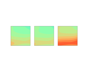
The resulting skewness and kurtosis as functions of  $\tanh {(k_ph)}$ and JONSWAP
  $\gamma$, for three different directional spreadings, are shown in figure 3. The first and second rows in figure 3 show skewness and kurtosis normalized by
  $\epsilon$ and
  $\epsilon ^2$, respectively, while the third row shows the ratio of kurtosis to skewness squared,
  $\lambda _4/\lambda _3^2$.

Figure 3. Exact (a–c) normalized skewness  $\lambda _3/\epsilon$ and (d–f) normalized kurtosis
  $\lambda _4/\epsilon ^2$, as well as (g–i) the ratio
  $\lambda _4/\lambda _3^2$, as functions of
  $\tanh {(k_ph)}$ and JONSWAP
  $\gamma$, for three different directional spreadings (from left to right,
  $\sigma _{\theta }=10^\circ$,
  $20^\circ$,
  $40^\circ$, corresponding to
  $n\approx 32$,
  $n\approx 7$ and
  $n\approx 1$, in the
  $\cos ^n{\theta }$ directional distribution).
It is observed that both skewness and kurtosis increase with decreasing water depth. Interestingly, the dependence of the frequency bandwidth controlled by JONSWAP  $\gamma$ is different in deep and shallow water: in deep water, the skewness and kurtosis are larger for broader spectra (smaller
  $\gamma$), while in more shallow water, the kurtosis and skewness increase with increasing
  $\gamma$. Both kurtosis and skewness decrease with larger directional spreading. It is worth noting that the ratio of kurtosis to skewness squared,
  $\lambda _4/\lambda _3^2$, is close to 2 (approximately within
  ${\pm }10\,\%$) over the full range of spectral parameters considered.
Here, we have considered a JONSWAP spectrum since this is probably the most commonly used model spectrum, in a wide range of engineering applications. However, it should be mentioned that real ocean spectra do not follow a perfect JONSWAP shape, although it has proven to be a good model in many ocean regions (Mazzaretto, Menéndez & Lobeto Reference Mazzaretto, Menéndez and Lobeto2022). The present numerical approach is, however, general, and can be applied to any type of wave spectrum, and a natural application of the present approach would be to obtain the skewness and kurtosis directly from more general types of wave spectra, e.g. for multimodal spectra describing simultaneous wind sea and swell, measured wave spectra or spectra predicted by operational spectral wave forecasting models (e.g. WAM, WAVEWATCH III). In this way, direct information about skewness and kurtosis, and hence associated statistical distributions of e.g. crest heights or wave heights, could be obtained without needing to rely on a few integrated parameters.
As a test of the robustness of the results obtained for JONSWAP spectra, skewness and kurtosis were calculated for 100 directional spectra taken from an operational wave forecasting model, and compared with the corresponding results obtained from the best-fit JONSWAP spectrum on the form (4.1a,b). The results are shown in figure 4. As seen from the figure there is relatively good agreement between these two approaches, which indicates that the results obtained for JONSWAP spectra may be applicable also for more general types of spectra. The spectra considered in figure 4 were chosen as the 100 largest sea states (largest significant wave-height) during a three-year period in a North-Sea location.

Figure 4. (a) Skewness  $\lambda _3$ and (b) kurtosis
  $\lambda _4$, estimated directly from 100 empirical wave-model spectra compared to results obtained for the corresponding best-fit JONSWAP spectra.
4.1. Accuracy of existing parametrizations
Based on the exact calculations of skewness and kurtosis shown in figure 3, the accuracy of the existing parametrizations that were summarized in § 2.1 are evaluated. The errors in per cent associated with the different parametrizations are shown in figures 5–10. As expected, the existing parametrizations are generally reasonably accurate within the range of parameters for which they were developed (see table 1), but in some cases are highly inaccurate outside these regions.

Figure 5. Error (in per cent) in estimated skewness and kurtosis for the narrow-band approximation (2.5a,b) with  $\varDelta =\varDelta _{1D}$.

Figure 6. Error (in per cent) in estimated skewness and kurtosis for the narrow-band approximation (2.5a,b) with  $\varDelta =\varDelta _{PS}$.

Figure 7. Error (in per cent) in estimated skewness and kurtosis for the parametrizations of Vinje & Haver (Reference Vinje and Haver1994).

Figure 8. Error (in per cent) in estimated skewness and kurtosis for the parametrizations from Jha & Winterstein (Reference Jha and Winterstein2000).

Figure 9. Error (in per cent) in estimated skewness for the Tayfun–Forristall approximation (Tayfun Reference Tayfun2006).

Figure 10. Error (in per cent) in estimated kurtosis for the parametrization from Annenkov & Shrira (Reference Annenkov and Shrira2014).
Based on the discussion in § 2.1.1, we have considered both choices of the coefficient  $\varDelta$ in the narrow-band approximation, i.e.
  $\varDelta =\varDelta _{1D}$ (Janssen Reference Janssen2009) and
  $\varDelta =\varDelta _{PS}$ (Pezzutto & Shrira Reference Pezzutto and Shrira2023). The prediction errors for these two forms of the narrow-band limit are shown in figures 5 and 6, respectively. It is seen that both forms of the narrow-band limit are quite accurate for deep water (the two forms coincide for infinite depth), but they have larger errors in more shallow water. As also indicated by the results in figure 1, using
  $\varDelta =\varDelta _{PS}$ leads to larger values of skewness and kurtosis compared to using
  $\varDelta =\varDelta _{1D}$, with the consequence that for most conditions, the narrow-band limit with
  $\varDelta =\varDelta _{1D}$ underestimates the real skewness and kurtosis, while
  $\varDelta =\varDelta _{PS}$ leads to overestimation.
It should be noted that when comparing the narrow-band limits with results for finite bandwidth spectra, it is not a priori clear how to best define the wavenumber appearing in the narrow-band limits. Here, we have used the peak wavenumber of the JONSWAP spectrum, but it may be that other choices of this wavenumber may improve the accuracy of the narrow-band limits. Some discussion on this can be found in § 3.3 in Janssen (Reference Janssen2017).
The accuracy of the expressions (2.10a,b) presented in Vinje & Haver (Reference Vinje and Haver1994) is shown in figure 7. As seen from the figure, their estimate for the skewness is relatively good for quite deep water ( $k_ph$ larger than approximately 1), but it overestimates significantly in more shallow water. For the kurtosis, the accuracy is also best for deep water, but consistently overestimates the exact values, extremely so in shallow water. Consistent with the assumptions made in Vinje & Haver (Reference Vinje and Haver1994), the error is smallest for
  $\gamma \approx 1$ and narrow directional spreading.
The accuracy of the parametrizations of Jha & Winterstein (Reference Jha and Winterstein2000) is shown in figure 8. The results from Winterstein & Jha (Reference Winterstein and Jha1995) are very similar, but are not shown here. These parametrizations were developed for unidirectional waves, for different values of JONSWAP  $\gamma$ and water depths. The expression for the skewness (2.13) is quite accurate for relatively deep water as long as the directional spreading is not too broad. The accuracy is less good for shallow water, where the correct skewness is underestimated up to about 80 %. For the kurtosis, the fit is consistently lower than the correct values, which is likely explained by the fact that third-order effects necessary for a consistent estimate of kurtosis to
  $O(\epsilon ^2)$ were not included in the analysis of Winterstein & Jha (Reference Winterstein and Jha1995) and Jha & Winterstein (Reference Jha and Winterstein2000).
The accuracy of the Tayfun–Forristall approximation for the skewness, shown in figure 9, is mostly within 30 % of the correct skewness, except for the broadest directional spreading in relatively shallow water depth where it overestimates up to 70 %. Note that also this approximation is consistently conservative.
Finally, the accuracy of the fit for the kurtosis presented in Annenkov & Shrira (Reference Annenkov and Shrira2014) is shown in figure 10. This fit was developed for infinitely deep water and for a specific frequency-dependent directional spreading function. It should be noted that this fit also includes the dynamical kurtosis, and is therefore not directly comparable to the other results discussed here. Nevertheless, it is seen that this parametrization is reasonably accurate for broad spectra ( $\gamma$ closer to 1) in deep water.
4.2. New parametrizations for skewness and kurtosis
Although the exact skewness and kurtosis can be calculated relatively efficiently for any spectrum using the method described in § 3, for many applications it is useful to have simple explicit formulas that enable easy estimation of the skewness and kurtosis. As documented in the previous subsection, none of the existing parametrizations provides accurate representations over the entire range of sea-state conditions encountered in typical ocean engineering applications. Therefore, by using the dataset of exact skewness and kurtosis values described above, the following expressions were fitted:
 $$\begin{gather} \lambda_3=(2.89 + 1.19\xi^{3.3} -0.28\nu^{0.8} + 0.35\xi^{2.9}\nu^{1.1})(1 + 1.42\zeta - 3.81\zeta^2 + 2.25\zeta^3)\epsilon, \end{gather}$$
 $$\begin{gather}\lambda_4= (2.34 - 0.31\xi)\lambda_3^2, \end{gather}$$
where
 \begin{equation} \xi = (k_ph)^{-1},\quad \nu = \ln{\gamma},\quad \zeta = \sin{\sigma_{\theta}}. \end{equation}
The accuracy of the parametrizations (4.4) is shown in figure 11, showing that they are accurate over a wide range of sea-state parameters. In the fitting of the expressions (4.4), a priority was to have good accuracy for realistic sea-state parameters, e.g. for common directional spreading parameters in the range of  $\sigma _{\theta }$ between
  $15^\circ$ and
  $35^\circ$.

Figure 11. Error (in per cent) in estimated skewness and kurtosis for the parametrization suggested in this paper, (4.4).
Generally, it is shown that the expressions (4.4) predict the skewness and kurtosis within about 5 % accuracy for typical realistic sea-state conditions in deep and intermediate water depths. It is worth noting the simple parametrization for the kurtosis, which for infinite depth reduces to the very simple approximation  $\lambda _4=2.34\lambda _3^2$.
5. Comparison to model tests and phase-resolved simulations
In the following, we compare the exact integral expressions for skewness and kurtosis with results from model tests of mechanically generated waves in a directional wave basin and results from phase-resolved numerical simulation using a nonlinear wave model based on the higher-order spectral method (HOSM) (Dommermuth & Yue Reference Dommermuth and Yue1987; West et al. Reference West, Brueckner, Janda, Milder and Milton1987).
The model tests were carried out in the Hydrodynamics Laboratory at Imperial College London in a directional wave basin having width 20 m and length 10 m, and water depth  $h=1.25$ m. A model-scale 1 : 100 is assumed so that the full-scale water depth is
  $h=125$ m. The model tests include eleven different sea states with different significant wave heights
  $H_s$ and peak periods
  $T_p$, generated according to a JONSWAP spectrum with a directional distribution in the form of a normal distribution with standard deviation
  $\sigma _{\theta }$. For one of the sea states, three different directional spreadings were considered (
 $\sigma _{\theta }=9^\circ$,
  $18^\circ$ and
  $27^\circ$), while the remaining sea states were run for
  $\sigma _{\theta }=18^\circ$. Each test was repeated about 60 times with different random amplitudes and phases. The duration of each repetition was about three hours full-scale, i.e. a total duration about 180 hours in each sea state. Skewness and kurtosis were estimated for each repetition from the time series of surface elevation, which was measured 5 m from the wave paddle, corresponding to a distance 500 m full scale. For some additional information on the model tests, see Gramstad, Johannessen & Lian (Reference Gramstad, Johannessen and Lian2023).
In addition to the model-test results, the same sea states were simulated with the HOSM. The nonlinear order in HOSM was set to  $M=3$, consistent with the order to which the integral expressions for skewness and kurtosis are valid. The HOSM simulations were initialized with the same directional JONSWAP spectra as used for the model tests. For each sea state, the wave field was simulated in a periodic domain with dimensions
  $16\lambda _p \times 16\lambda _p$ for duration 25 min, where the first five minutes were discarded due to possible transient startup effects. It was observed that for the remaining 20 min of the simulations, the skewness and kurtosis were close to stationary, and for each seed, the skewness and kurtosis were estimated over the entire computational domain in space and the 20 min duration in time. For each sea state, 50 repetitions were run, with different random amplitudes and phases each repetition. Some testing was carried out to ensure that the HOSM results were not affected significantly by choice of computational domain, discretization of the spectrum, and so on.
The resulting estimates of skewness and kurtosis, compared to the exact values calculated from (3.1a,b), are shown in figure 12. Results from the proposed parametrization (4.4) are also included in the figure. The sea states in figure 12 are sorted in order of increasing sea-state steepness  $k_p\sqrt {m_0}$. For the model tests, the boxes and whiskers show the variation over approximately 60 random repetitions of each sea state. Here, the boxes cover the range from the first to the third quartile, and the whiskers show the entire range of the data. For the HOSM results, the whiskers indicate
  $\pm$ one standard deviation of the skewness and kurtosis estimated from the individual repetitions of the same sea state. Naturally, the HOSM estimates are associated with smaller statistical uncertainty than the model-test results since the HOSM estimates are based on an average over a large area in space and time, while the model-test results are based on single-point time series only.

Figure 12. (a) Skewness  $\lambda _3$ and (b) excess kurtosis
  $\lambda _4$ from model tests and HOSM simulations compared to ‘exact’ values as well as results from the new parametrization suggested in this paper, (4.4).
As seen from figure 12, there is quite good agreement between model-test results, the HOSM and the exact values, except for the two steepest sea states, where there is a significant contribution from wave breaking in the model tests. In these sea states, the validity of the HOSM is also more questionable. In fact, in these sea states, occasional failures of the HOSM simulations were observed, due to numerical instabilities arising from too steep waves. In such steep sea states, ideally the HOSM should be accompanied by a breaking model, as discussed in e.g. Gramstad et al. (Reference Gramstad, Johannessen and Lian2023). With the exception of these two steepest sea states, there is good agreement between the exact skewness and kurtosis and the HOSM estimates. It should be noted that obtaining the skewness and kurtosis from short crested HOSM simulation is significantly more computationally heavy than evaluating the integrals (3.1a,b). Further, it should be noted that both the HOSM and model-test results in principle include contributions to the dynamical kurtosis. In this sense, the close agreement between HOSM and the exact values for the bound kurtosis suggests that the contribution from the dynamical kurtosis is quite small in the cases considered here.
Another point that should be mentioned is that the spectrum in both HOSM simulations and model-tests evolves with time, so that the actual spectral shapes after some time, or some distance down the wave basin, deviate from the target JONSWAP spectrum on which the exact calculations are based. We stress that in addition to being much more computationally efficient and not affected by statistical uncertainty, the direct solution of the integrals for skewness and kurtosis has the advantage of not having to deal with non-stationary statistics and non-stationary spectra in phase-resolved simulation.
6. Application to crest height distributions
As mentioned in the Introduction, the skewness and kurtosis appear as parameters in the theoretical higher-order statistical distributions for surface elevation, wave heights and crest heights. In the following, we will focus on the third-order crest distribution in the form given by Tayfun & Fedele (Reference Tayfun and Fedele2007), which in terms of its cumulative distribution function  $F(\zeta )$ can be written in the form
 \begin{equation} 1 - F(\zeta) = P\left(\frac{\eta_c}{H_s}>\zeta\right)= \exp{(-8\chi^2)}\left[1+\frac{8}{3}\,\lambda_4\zeta^2(4\zeta^2-1)\right]\!, \end{equation}
where  $\chi$ is given by the quadratic equation
  $\zeta =\chi + 2\lambda _3\chi ^2/3$. If we set
  $\lambda _4=0$ and approximate
  $\lambda _3$ by the Tayfun–Forristall approximation discussed in § 2.1.4, then this reduces to the crest distribution of Tayfun (Reference Tayfun2006), which has also been adopted in recent crest distributions developed in the LOADS joint industry project (JIP) (Gibson Reference Gibson2021; Karmpadakis & Swan Reference Karmpadakis and Swan2022). Note that Gibson (Reference Gibson2021) and Karmpadakis & Swan (Reference Karmpadakis and Swan2022) include also terms to account for effects beyond second order (as well as corrections to account for wave breaking as discussed below). These corrections are, however, empirical and not based on theoretical derivations, as is the case for the terms involving
  $\lambda _4$ in the Tayfun–Fedele model (6.1).
To evaluate the effect of using the exact skewness and kurtosis in the crest height models, the Tayfun–Fedele model (6.1) with  $\lambda _3$ and
  $\lambda _4$ from exact calculations as well as from the parametrization (4.4) are shown in figure 13 for nine of of the model-test sea states considered in § 5. The two steepest sea states, which are affected strongly by wave breaking, are not shown. The empirical crest distributions from both model tests and HOSM simulation are also plotted, together with various other relevant crest height distributions: the Rayleigh distribution for crest heights, the Forristall crest distribution (Forristall Reference Forristall2000), the second-order Tayfun model with
  $\lambda _3$ approximated by the Tayfun–Forristall approximation (Tayfun Reference Tayfun1980, Reference Tayfun2006), as well as the recent crest distribution suggested in the LOADS JIP (Gibson Reference Gibson2021), referred to as LOADS-OCG in the following.

Figure 13. Distributions of crest heights from model tests, HOSM simulations and the Tayfun–Fedele model with exact skewness and kurtosis, as well as other relevant crest height distributions.
In order to be able to distinguish the different distributions visually, as well as to exclude the effect of wave breaking (which, with the exception of the LOADS-OCG crest height model, is not included in any of the approaches considered here), the distributions are plotted for a smaller range of exceedance probabilities limited by  $10^{-3}$, or at the probability level for which the generalized Pareto wave breaking tail model starts in the LOADS-OCG model, in the case that this happens for exceedance probabilities above
  $10^{-3}$.
From figure 13, it is first noted that the results obtained with exact  $\lambda _3$ and
  $\lambda _4$, and from the new parametrization (4.4), are practically identical (in practice, the difference is not visible in the figure), confirming the accuracy of (4.4). Further, it is observed that the Tayfun–Fedele model (6.1) with exact
  $\lambda _3$ and
  $\lambda _4$ is in all sea states in very good agreement with the crest heights from the HOSM simulations. For the model tests, the results show some qualitative variations from sea state to sea state, some of which are not explained readily. For example, in the sea state
  $H_s=14.2$ m,
  $T_p=16.7$ s, the model tests are clearly above all other results, while in the quite similar sea state
  $H_s=15.0$ m,
  $T_p=18.3$ s, the model tests are clearly lower than the third-order based models. This may be explained by uncertainties and inaccuracies in the wave-tank measurements. However, overall it is observed that the model-test results are in best agreement with the approaches that include third-order effects (the Tayfun–Fedele model with non-zero kurtosis, HOSM simulations and LOADS-OCG model). In fact, especially in the steeper sea states, the LOADS-OCG model seems to be in best agreement with the model-test results. To some extent this may be expected considering that the higher-order term in the LOADS-OCG model is fitted to model tests. Interestingly, the HOSM results are, however, in somewhat better agreement with the Tayfun–Fedele model than the LOADS-OCG model. However, the differences between the approaches considering third-order effects are generally relatively small. The models based on second-order only (Forristall, Tayfun–Fedele with
  $\lambda _4=0$) are generally underestimating both HOSM simulations and the model tests.
In the context of the discussion in § 4.1, where the accuracy of different parametrizations of skewness and kurtosis was presented in terms of the percentage error, it should be noted that to what extent a given error in skewness and kurtosis is significant will depend on the specific application of interest. In order to illustrate this point, in figure 14 we have shown the error in the Tayfun–Fedele crest distribution as function of the corresponding error in kurtosis and skewness used in the model. As an example, an overestimation of 50 % in both skewness and kurtosis leads to an overestimation of the crest height at the  $10^{-3}$ level of about 10 %.

Figure 14. The errors at (a) the  $10^{-3}$ level and (b) the
  $10^{-5}$ level in the Tayfun–Fedele (TF) crest distribution functions of error in estimates of skewness and kurtosis used in the model. Here, a sea state with
  $H_s=10$ m,
  $T_p=12.5$ s at 125 m water depth is used.
7. Conclusions
In this paper, a numerical method for calculating the exact surface elevation skewness and kurtosis due to second- and third-order non-resonant nonlinear interactions, for an arbitrary wave spectrum, has been presented and validated. It is shown that the present numerical approach enables efficient calculation of skewness and kurtosis, and hence represents an efficient alternative to e.g. phase-resolved time domain Monte Carlo simulations. It is shown that none of the parametrizations of skewness and kurtosis that are reported in the existing literature are accurate over the entire range of sea-state parameters that are encountered in realistic ocean conditions. New parametrizations for skewness and kurtosis, as functions of wave steepness, water depth, spectral bandwidth and directional spreading, have therefore been presented, and it is shown that they represent a significant improvement over existing alternatives.
It is suggested that using the exact skewness and kurtosis, or the accurate parametrization suggested here, in theoretical higher-order distributions for crest heights, wave heights and surface elevation, represents the most natural way to include the effects of nonlinearity in the statistical distributions of the ocean surface. It should be noted, however, that these theoretically based crest distributions will overestimate wave crests in steep sea states, if no correction due to wave breaking is applied. Hence, for consistent statistical distributions over all realistic ocean conditions, these models should be extended with some correction for wave breaking, e.g. by using an approach similar to the one adopted by Gibson (Reference Gibson2021).
Finally, it should be mentioned that although only JONSWAP-type spectra were considered here, the present numerical approach is general and can be applied to any type of wave spectrum. A natural application of the present approach would be to obtain the skewness and kurtosis directly from more general types of wave spectra, e.g. for multimodal spectra describing simultaneous wind sea and swell, measured wave spectra or spectra predicted by operational spectral wave forecasting models (e.g. WAM, WAVEWATCH III). In this way, direct information about skewness and kurtosis, and hence associated statistical distributions of e.g. crest heights or wave heights, could be obtained without needing to rely on a few integrated parameters.
Acknowledgements
We would like to thank the reviewers for several useful comments, and in particular one of the reviewers for pointing out a flaw in the original version related to the handling of the mean flow in calculation of the skewness and kurtosis. We would further like to thank Dr M.A. Tayfun for useful information on the different narrow-band limits of the skewness and kurtosis, and Dr E. Bitner-Gregersen and Dr A. Nestegård for several useful comments on draft versions of the paper.
Declaration of interests
The authors report no conflict of interest.
Appendix A. Proof for explicit dependence of sea-state steepness
By introducing a change of variables from  $\boldsymbol {k}$ to
  $\tilde {\boldsymbol {k}}=\boldsymbol {k}/k_p$ in (2.3a,b), and defining a normalized spectrum
  $\tilde {E}(\tilde {\boldsymbol {k}})=k_p^2\,E(k_p\tilde {\boldsymbol {k}})/m_0$, (2.3a,b) can be written as
 $$\begin{gather} \lambda_3=3\epsilon\int \tilde{E}(\tilde{\boldsymbol{k}}_1)\,\tilde{E}(\tilde{\boldsymbol{k}}_2)\,K^{(3)}(\tilde{\boldsymbol{k}}_1, \tilde{\boldsymbol{k}}_2)\,\textrm{d}\tilde{\boldsymbol{k}}_{1,2}, \end{gather}$$
 $$\begin{gather}\lambda_4=12\epsilon^2\int \tilde{E}(\tilde{\boldsymbol{k}}_1)\,\tilde{E}(\tilde{\boldsymbol{k}}_2)\,\tilde{E}(\tilde{\boldsymbol{k}}_3)\,K^{(4)} (\tilde{\boldsymbol{k}}_1, \tilde{\boldsymbol{k}}_2, \tilde{\boldsymbol{k}}_3)\,\textrm{d}\tilde{\boldsymbol{k}}_{1,2,3}, \end{gather}$$
where  $\epsilon =k_p\sqrt {m_0}$, and we use the fact that the kernel functions possess the properties
 \begin{equation} K^{(3)}(\boldsymbol{k}_1, \boldsymbol{k}_2)=k_p\,K^{(3)}(\tilde{\boldsymbol{k}}_1, \tilde{\boldsymbol{k}}_2),\quad K^{(4)}(\boldsymbol{k}_1, \boldsymbol{k}_2, \boldsymbol{k}_3)=k_p^2\,K^{(4)}(\tilde{\boldsymbol{k}}_1, \tilde{\boldsymbol{k}}_2, \tilde{\boldsymbol{k}}_3). \end{equation}
Thus for any spectrum that in normalized form does not depend on  $\epsilon$, the dependence of steepness can be factored out. For example, for the JONSWAP spectrum (i.e.
  $E(\boldsymbol {k})$ corresponding to (4.1a,b)), it can be shown that
  $\tilde {E}(\tilde {\boldsymbol {k}})$ depends only on
  $\gamma$ and directional spreading parameter
  $n$.
$n$.


