


1. Introduction
The stability problem of a liquid film flowing down an inclined or vertical plane is of increasing importance owing to its widespread applications in various areas of applied science and engineering, such as in heavy casting technology, precision coating, laser cutting processes and the processes of paint finishing, etc. A microscopic instability can cause catastrophic conditions for the film flow problems, therefore it is desirable to investigate this flow problem properly and accurately for making successful designs of fluid devices so that homogeneous fluid flow as per the required conditions can be made. Here, it is important to mention that enormous mathematical calculations, as well as various numerical programs that are required for exploring this type of flow problem theoretically or experimentally, must be correct.
Kapitza & Kapitza (Reference Kapitza and Kapitza1949) were the first to investigate experimentally the wave motions of a viscous fluid layer flowing down a vertical cylinder, where they recorded the existence of several wavy regimes, including a series of nearly solitary waves. After this pioneering work, several experimental studies on liquid films flowing down an inclined or vertical plane under various conditions have been carried out by many researchers (e.g. Ishihara, Iwagaki & Ishihara Reference Ishihara, Iwagaki and Ishihara1952; Greenberg Reference Greenberg1956; Binnie Reference Binnie1957, Reference Binnie1959; Fulford Reference Fulford1964; Massot, Irani & Lightfoot Reference Massot, Irani and Lightfoot1966; Whitaker & Jones Reference Whitaker and Jones1966; Liu, Paul & Gollub Reference Liu, Paul and Gollub1993; Liu & Gollub Reference Liu and Gollub1994; and the references therein). Benjamin (Reference Benjamin1957) was the first to investigate theoretically the linear instability of a liquid film flowing down an inclined plane being bounded on the other side by a free surface. Yih (Reference Yih1963) presented Benjamin's theoretical results in more simplified forms by considering separately the limits of small Reynolds and small wavenumber. In these analyses, they derived the stability criterion in terms of Reynolds number  $Re$ and angle of inclination
  $\theta$, which fairly agrees with the experimental results for small values of
  $\theta$ (Alekseenko, Nakoryakov & Pokusaev Reference Alekseenko, Nakoryakov and Pokusaev1994).
Finite-amplitude wave solutions and nonlinear stability analysis of a viscous liquid film flowing down an inclined plane were initiated by Benney (Reference Benney1966). He derived the free-surface evolution equation in terms of film thickness by employing the long-wave expansion method (small Reynolds number approach). Following Benney's analysis, investigation of the long-wave surface evolution equations for various orders of  $Re$ and
  $We$ can be found in the works of Gjevik (Reference Gjevik1970), Lin (Reference Lin1974), Chang (Reference Chang1989) and Pumir, Manneville & Pomeau (Reference Pumir, Manneville and Pomeau1983), among others. By contrast, the large Reynolds number approach (momentum-integral method) has been employed by Prokopiou, Cheng & Chang (Reference Prokopiou, Cheng and Chang1991) and Lee & Mei (Reference Lee and Mei1996) to examine the instability of a viscous liquid film flowing down an inclined plane. It is noticeable that all the above studies are restricted to a definite value of
  $\theta$ or in a specific range of
  $\theta$ in which
  $\theta$ is small. Recently, using the momentum-integral method, Dholey & Gorai (Reference Dholey and Gorai2021) examined thoroughly the linear and nonlinear stability analysis of a viscous liquid film falling down an inclined plane for the full range of the inclination angle
  $\theta$ (
 $0 < \theta \le 90^{\circ }$).
Flow of an electrically conducting liquid film has several practical applications, such as in nuclear energy equipment, different cooling systems and laser cutting processes (Glukhikh, Tananaev & Kirilov Reference Glukhikh, Tananaev and Kirilov1987; Blum, Mayorov & Tsebers Reference Blum, Mayorov and Tsebers1989). The effects of an electric field on the falling film problems have been found in the works of Rohlfs et al. (Reference Rohlfs, Cammiade, Rietz and Scheid2021), Papageorgiou (Reference Papageorgiou2019), Tseluiko & Papageorgiou (Reference Tseluiko and Papageorgiou2006), Wray, Matar & Papageorgiou (Reference Wray, Matar and Papageorgiou2017), and the references therein. Conroy & Matar (Reference Conroy and Matar2017) investigated the stability of three-dimensional ferrofluid films in a magnetic field. However, there exist many recently published papers on linear and nonlinear stability analysis of an electrically conducting liquid film falling down an inclined or vertical plane. Here, we mention those by Gonzalez & Castellanos (Reference Gonzalez and Castellanos1996), Korsunsky (Reference Korsunsky1999), Dandapat & Mukhopadhyay (Reference Dandapat and Mukhopadhyay2003), Mukhopadhyay, Dandapat & Mukhopadhyay (Reference Mukhopadhyay, Dandapat and Mukhopadhyay2008) and Dholey (Reference Dholey2017). Among these studies, only Mukhopadhyay et al. (Reference Mukhopadhyay, Dandapat and Mukhopadhyay2008) considered the momentum-integral method for investigating the problem under a fixed value  $\theta =75^{\circ }$. The nonlinear evolution equation (4.5) of our present study may be the same as the corresponding equation
  $(19)$ in Mukhopadhyay et al. (Reference Mukhopadhyay, Dandapat and Mukhopadhyay2008), but the results obtained from figures 3–8 of their analysis are not correct, as the curves
  $k_c$ and
  $k_s$ (in those figures) do not follow the known relation
  $k_c =2 k_s$ (Dholey & Gorai Reference Dholey and Gorai2021). Dandapat & Mukhopadhyay (Reference Dandapat and Mukhopadhyay2003) have shown the existence of two critical values of
  $M$, namely,
  $M_c$ and
  ${\bar M}_c$, in figure 3 of their analysis. The value of
  ${\bar M}_c$ (analogous to
  $M_j$) is not correct as the curve
  $J_2 =0$ decreases continuously with the increase of
  $M$ (see figures 17 and 18). For this, the present authors claim that the results of Dandapat & Mukhopadhyay (Reference Dandapat and Mukhopadhyay2003) and Mukhopadhyay et al. (Reference Mukhopadhyay, Dandapat and Mukhopadhyay2008) are of doubtful validity.
The aim of this study is therefore to extend the work of Dholey & Gorai (Reference Dholey and Gorai2021) by considering the flow of an electrically conducting liquid film down an inclined plane in the presence of an electromagnetic field. The linear stability analysis reveals that the magnetic parameter  $M$ has a stabilizing influence up to the value
  $E \approx 2.45$, independent of
  $\theta$, and after this value of
  $E$, the (slowly) destabilizing influence of
  $M$ has been found up to the value
  $M \approx 0.73635$, and then continuously follows the stabilizing influence. Here, our main interest in the nonlinear stability analysis is discussed by showing all four possible distinct flow zones of this problem in
  $Re$–
$Re$– $k$,
$k$,  $\theta$–
 $k$,
$k$,  $E$–
$E$– $k$ and
  $M$–
$M$– $k$ planes. The value of
  $M_j$ (analogous to
  ${\bar M}_c \approx 1.253$ of Dandapat & Mukhopadhyay Reference Dandapat and Mukhopadhyay2003) is obtained numerically as
  $M_j \approx 3.99730$, independent of the values of
  $E$,
$E$,  $Re$ and
  $\theta$. The novelty of this analysis is the existence of a new explosive unstable zone that arises only in the presence of a magnetic field depending upon the values of the other parameters. The physical reason for this fact has been confirmed by delineating the curves
  $\omega _i^+$ and
  $J_2$ against
  $k$ for several values of
  $M$, since the demarcations of different flow zones of this problem depend essentially on the values (positive or negative) of
  $\omega _i^+$ and
  $J_2$. Various numerical results in the form of figures, especially the range of
  $k$ for different flow zones of this problem, are presented in the results and discussion sections of this paper to authenticate the solutions and to manifest the effectiveness of the proposed modelling. The non-availability of the experimental evidences does not allow us to compare our numerical results with the experimental predictions.
2. Mathematical formulation
We consider the two-dimensional gravity-driven flow of an electrically conducting viscous fluid layer of mean thickness  $h_0$ down an inclined plane of inclination
  $\theta$ (
 $0 < \theta \le 90^{\circ }$) with the horizon, in the presence of an electromagnetic field. We introduce a Cartesian coordinates system such that the
  $x$-axis coincides with the plane surface, and the
  $z$-axis points vertically upwards from this surface, as shown in figure 1. Here, the constant electric and magnetic fields are acting along the normal to the
  $x$–
$x$– $z$ and
  $x$–
$x$– $y$ planes, respectively.

Figure 1. Physical sketch of the problem.
The basic equations governing this flow problem are the continuity equation and the Navier–Stokes equations with the Lorentz (electromagnetic body) force  $\boldsymbol {J} \times \boldsymbol {B}$:
 $$\begin{gather} \boldsymbol{\nabla} \boldsymbol{\cdot} \boldsymbol{v} = 0, \end{gather}$$
 $$\begin{gather}\rho \left \{ \partial_t{\boldsymbol{v}} + {(\boldsymbol{v} \boldsymbol{\cdot} \boldsymbol{\nabla}) \boldsymbol{v}} \right \} =- \boldsymbol{\nabla} p + \mu\,\nabla^2 \boldsymbol{v} + \rho \boldsymbol{g} + {\boldsymbol{J} \times \boldsymbol{B}}, \end{gather}$$
where  $\boldsymbol {v} =(u, 0, w)$ and
  $\boldsymbol {g} =(g\sin \theta, 0, - g\cos \theta )$ are liquid film velocity and gravitational acceleration, respectively, and
  $p$,
$p$,  $\rho$ and
  $\mu$ are pressure, density and dynamic viscosity of the fluid, respectively. Here,
  $\boldsymbol {\nabla } =(\partial _x, 0, \partial _z)$, and
  ${\nabla }^2$ is the Laplacian with respect to
  $x$ and
  $z$. The current density
  $\boldsymbol {J}$ is given by Ohm's law, without the Hall effect as (Shercliff Reference Shercliff1965)
 \begin{equation} \boldsymbol{J} = \sigma (\boldsymbol{E} + \boldsymbol{v} \times \boldsymbol{B}), \end{equation}
where  $\sigma$ is the electrical conductivity of the fluid. The above magnetic and electric fields (
 $\boldsymbol {B}$ and
  $\boldsymbol {E}$) are defined by Maxwell's equations as
 \begin{equation} \boldsymbol{\nabla} \boldsymbol{\cdot} \boldsymbol{B} = 0, \quad \boldsymbol{\nabla} \times \boldsymbol{B} = \mu_e \boldsymbol{J} \quad \text{and} \quad \boldsymbol{\nabla} \times \boldsymbol{E} =- \partial_t \boldsymbol{B}, \end{equation}
where  $\mu _e$ is the magnetic permeability. We neglect the displacement current in Maxwell's equations since we are not concerned with the consequences that are related in any way to the propagation of electromagnetic waves (Chandrasekhar Reference Chandrasekhar1961). As the magnetic Reynolds number is small, one can obtain the electric and magnetic fields as
  $\boldsymbol {E} =E_0$ and
  $\boldsymbol {B} =B_0$, respectively (Mukhopadhyay et al. Reference Mukhopadhyay, Dandapat and Mukhopadhyay2008; Dholey Reference Dholey2016, Reference Dholey2017; and the references therein).
The boundary conditions related to this flow problem are
 \begin{equation} \boldsymbol{v} = 0 \quad \text{at }z = 0 \quad (\text{no-slip condition}). \end{equation}
We define the perturbed interface as  $F(x, z, t) =z-h(x, t)$, and then the kinematic condition on the free surface is obtained as (see figure 1)
 \begin{equation} \frac{{\rm D}F}{{\rm D}t} = \partial_t h + \boldsymbol{v} \boldsymbol{\cdot} \boldsymbol{\nabla} (h - z) = 0 \quad \text{at }z = h(x,t), \end{equation}
where  ${\rm D}/{\rm D}t$ is the total derivative of the film thickness with respect to time
  $t$. Here, the dynamic influence of gas above the liquid film is neglected, and the effect of surface tension is included for which the tangential stress vanishes and the normal stress just balances with the surface tension:
 $$\begin{gather} \boldsymbol{\tau}\boldsymbol{\cdot} \boldsymbol{n}\boldsymbol{\cdot} \boldsymbol{t} = 0 \quad \text{at } z = h(x,t), \end{gather}$$
 $$\begin{gather}p_0 + ({\boldsymbol{\tau}\boldsymbol{\cdot}\boldsymbol{n}})\boldsymbol{\cdot}{\boldsymbol{n}} =- \sigma_0\,{\boldsymbol{\nabla}\boldsymbol{\cdot}\boldsymbol{n}} \quad \text{at } z = h(x,t), \end{gather}$$
where  $\boldsymbol {n} =(- h_x, 1, 0)/\sqrt {1+h_x^2}$ and
  $\boldsymbol {t} =(1, h_x, 0)/ \sqrt {1+h_x^2}$ are the outward-drawn unit normal and unit tangent vectors to the interface, respectively. Also,
  $\boldsymbol {\tau } = -pI + 2\mu \boldsymbol {e}$ is the stress tensor, where
  $\boldsymbol {e} = ({\boldsymbol {\nabla }\boldsymbol {v}} + \boldsymbol {\nabla }\boldsymbol {v}^{\rm T})/2$ is the rate-of-strain tensor, and
  $\boldsymbol {I}$ is the identity tensor. Moreover,
  $p_0$ is the pressure of the ambient gas and
  $\sigma _0$ is the surface tension coefficient.
To rewrite the basic equations and the boundary conditions in dimensionless form, we introduce the dimensionless variables with a bar sign as
 \begin{align} x = l_0{\bar x},\quad (h,z) = h_0({\bar h}, {\bar z}),\quad t = (l_0/u_0){\bar t},\quad u = u_0 {\bar u},\quad w = (u_0h_0/l_0){\bar w},\quad p = (\rho u_0^2){\bar p,} \end{align}
where we consider  $l_0$ as the characteristic longitudinal length scale whose order may be considered the same as the wavelength,
  $h_0$ as the length scale in the transverse direction and the Nusselt velocity
  $u_0 =gh_0^2 \sin \theta /3\nu$ as the velocity scale along the longitudinal direction.
Using (2.9a–f) in (2.1)–(2.8), removing the bar sign over the variables, and retaining the terms up to  $O(\epsilon )$, we obtain the reduced governing hydromagnetic equations as
 $$\begin{gather} u_x + w_z = 0, \end{gather}$$
 $$\begin{gather}\epsilon\,Re \left( u_t + u u_x + w u_z \right) =- \epsilon\,Re\,p_x + u_{zz} + 3 + M^2(E - u), \end{gather}$$
 $$\begin{gather}0 =- Re\,p_z - 3 \cot\theta + \epsilon w_{zz}. \end{gather}$$
The reduced boundary conditions at the plate surface ( $z = 0$) are
 \begin{equation} u = 0 \quad \text{and} \quad w = 0, \end{equation}
and on the free surface ( $z = h(x, t)$) are
 $$\begin{gather} w = h_t + u h_x, \end{gather}$$
 $$\begin{gather}u_z = 0 \end{gather}$$
and
 \begin{equation} p - p_a + \epsilon^2\,We\,h_{xx} = 0. \end{equation}
The dimensionless parameters associated with this problem are as follows:  $\epsilon = h_0/l_0$ is the aspect ratio, which is very small (
 $\ll 1$) as the fluid film is thin;
  $Re = u_0h_0/\nu$ is the Reynolds number, which measures the strength of the Nusselt flow;
  $M = B_0h_0{\sqrt {\sigma /\rho \nu }}$ is the Hartmann number, which measures the strength of the magnetic field;
  $E = E_0/(B_0u_0)$ is the electric parameter, which measures the strength of the electric field;
  $p_a = p_0/(\rho u_0^2)$ is the atmospheric pressure; and
  $We =\sigma _0/(\rho u_0^2 h_0)$ is the Weber number, which measures the surface tension.
Indeed, the strength of the parameters  $E$,
$E$,  $M$,
$M$,  $Re$ and
  $We$ can vary widely depending upon numerous factors, including the types of fluids, angle of inclination
  $\theta$, flow layer thickness
  $h_0$, source values of
  $B_0$ and
  $E_0$, and the specific conditions of the environment. However, to estimate the realistic physical values of the parameters
  $E$,
$E$,  $M$,
$M$,  $Re$ and
  $We$ for the most common electrically conducting fluids, such as mercury and liquid sodium, we have taken
  $g =9.8\ {\rm m}\ {\rm s}^{-2}$,
  $h_0 =0.6 \times 10^{-4}\ {\rm m}$,
  $\theta =45^{\circ }$,
  $E_0 =0.05\ {\rm V}\ {\rm m}^{-1}$ and
  $B_0 =0.5T$, and then computed the values of
  $E$,
$E$,  $M$,
$M$,  $Re$ and
  $We$ presented in table 1. It is well known that for mercury at
  $20\,^{\circ }{\rm C}$,
  $\rho =13545\ {\rm kg}\ {\rm m}^{-3}$,
  $\nu =1.147 \times 10^{-7}\ {\rm m}^2\ {\rm s}^{-1}$,
  $\sigma =1.04 \times 10^{6}\ {\rm S}\ {\rm m}^{-1}$ and
  $\sigma _0 =0.4865\ {\rm N}\ {\rm m}^{-1}$; and for liquid sodium at
  $400\,^{\circ }{\rm C}$,
  $\rho =856\ {\rm kg}\ {\rm m}^{-3}$,
  $\nu =2.840 \times 10^{-7}\ {\rm m}^2\ {\rm s}^{-1}$,
  $\sigma =2.50 \times 10^{6}\ {\rm S}\ {\rm m}^{-1}$ and
  $\sigma _0 =0.1610\ {\rm N}\ {\rm m}^{-1}$. Observing the values of
  $E$,
$E$,  $M$,
$M$,  $Re$ and
  $We$, we have assumed that
  $E \approx O(1) \approx M$,
  $Re \approx O(\epsilon ^{-1})$ and
  $We \approx O(\epsilon ^{-2})$.
Table 1. Values of  $E$,
$E$,  $M$,
$M$,  $Re$ and
  $We$ for different electrically conducting fluids.

The nonlinear system of equations (2.10)–(2.16) admits a steady basic solution  $(u, w) \equiv (U, 0)$, independent of
  $x$ and
  $t$, which is obtained as follows:
 \begin{equation} u(z) = \frac{1}{\delta_1}\left(\frac{m}{h}\right) U(Z), \end{equation}
where
 \begin{align} \left. \begin{gathered} U(Z) = \frac{a_0}{M^2} \left(1 - \frac{\cosh\{M(Z-1)\}}{\cosh(M)} \right), \quad m = \int_0^h u\,{\rm d}z = \frac{a_0h}{M^2} \left( 1 - \frac{\tanh(Mh)}{Mh} \right)\\ \text{and} \quad \delta_1 = \int_0^1 U(Z) \,{\rm d}Z = \frac{a_0}{M^2} \left(1 - \frac{\tanh M}{M} \right), \quad \text{with} \ a_0 = 3 + E M^2 \text{ and } Z = \frac{z}{h}. \end{gathered} \right\} \end{align}
Equations (2.11) and (2.18) confirm that the magnetic field can be applied without any electric field, but the electric field acts only in the presence of a magnetic field. In fact, the electromagnetic field in a fluid medium is the combination of an electric field with a magnetic field. For  $E =0$ and
  $M \rightarrow 0$,
  $U(Z) \rightarrow (3 Z - 1.5 Z^2)$ as well as
  $(m, \delta _1) \rightarrow (h^3, 1)$, which are exactly the same as the corresponding results reported by Dholey & Gorai (Reference Dholey and Gorai2021).
3. Momentum-integral equations
Integrating (2.12) and then using (2.16), we obtain the dimensionless pressure  $p(x, z, t)$ as
 \begin{equation} p = p_a -\epsilon^2\,We\,h_{xx} + 3\,Re^{-1} \cot\theta (h - z). \end{equation}
Integrating the continuity equation (2.10) and the  $x$-momentum equation (2.11), after using (3.1), with respect to
  $z$ from
  $0$ to
  $h$ by the Leibnitz rule, and using the boundary conditions (2.13a,b)–(2.15), we have
 $$\begin{gather} h_t + m_x = 0, \end{gather}$$
 $$\begin{gather}m_t + \alpha \left(\frac{m^2}{h}\right)_x = \epsilon^2\,We\,hh_{xxx} - \left( \frac {3\cot\theta}{Re}\right) hh_x + \frac{3h}{\epsilon\,Re} - \frac{Am}{\epsilon\,Re\,h^2} - \frac{M^2}{\epsilon\,Re } (E h - m), \end{gather}$$
where the expressions of the shape factors  $A$ and
  $\alpha$ are given by
 \begin{align} \left. \begin{gathered} A = \left(\frac{{\rm d}U}{{\rm d}Z}\right)_{Z=0} = M^2 \left( \frac{\tanh M}{M - \tanh M} \right) \quad \text{and} \quad \alpha = \frac{\delta_2}{\delta_1^2} = \frac{M}{2}\, \frac{3(M - \tanh M) - M \tanh^2M}{(M - \tanh M)^2}, \\ \text{with} \ \delta_2 = \int_0^1 U^2(Z) \,{\rm d}Z. \end{gathered} \right\} \end{align}
Equation (3.4) confirms that the shape factors  $A$ and
  $\alpha$ depend only on the values of
  $M$. For
  $M \rightarrow 0$,
  $(A, \alpha ) \rightarrow (3.0, 1.2)$, which are exactly the same as the values obtained by Dholey & Gorai (Reference Dholey and Gorai2021). The full range of
  $\alpha$ can be obtained as
  $1 \le \alpha \le 1.2$ since
  $\alpha \rightarrow 1$ as
  $M \rightarrow \infty$.
Equations (3.2) and (3.3) have a known solution
 \begin{equation} m_0 = \delta_1 = \frac{a_0}{M^2} \left(1 - \frac{\tanh M}{M} \right), \quad h = 1, \end{equation}
which is the Nusselt flat-film solution in the presence of an electromagnetic field, which has the property that as  $M\rightarrow 0$,
  $m_0\rightarrow 1$ irrespective of the values of
  $E$.
$E$.
4. Stability analysis
The results of both linear and nonlinear stability analysis will be deduced from the free surface evolution equation. To obtain the nonlinear evolution equation of this problem, we assume
 \begin{equation} h(x,t) = 1 + \eta(x, t) \quad \text{and} \quad m(x, t) = m_0 + {\bar m}(x, t), \end{equation}
where  $\eta \ll 1$ and
  ${\bar m} \ll 1$ are the dimensionless perturbations of the film thickness and flow rate, respectively. Substituting (4.1a,b) into (3.2) and (3.3), retaining the terms up to the second-order fluctuations, and then dropping the bar sign, we get
 \begin{gather} \eta_t + m_x = 0, \end{gather}
 $$\begin{gather} m_t + \alpha \left(2 m_0 m_x - m_0^2 \eta_x \right) - \epsilon^2\,We\,\eta_{xxx} + \left(\frac{3\cot \theta}{Re}\right)\eta_x - \left\{ \frac{9 + M^2(3E - 2m_0) } {\epsilon\,Re} \right\}\eta \nonumber\\ {}+ \frac{(A + M^2)m}{\epsilon\,Re} =- 2 m_t \eta - 2 \alpha (m m_x + m_0 m_x \eta - m_0 m \eta_x ) - \left(\frac{9\cot\theta}{Re}\right) \eta\eta_x \nonumber\\ {}+\left\{ \frac{9 + M^2(3E - m_0)}{\epsilon\,Re} \right\}\eta^2 - \left(\frac{2mM^2}{\epsilon\, Re}\right)\eta + 3\epsilon^2\,We\,\eta {\eta_{xxx}}. \end{gather}$$
Assuming  $O(m) =O(\eta ) =\epsilon$, we obtain the zeroth-order approximation from (4.3) as
 \begin{equation} m = c\eta \quad \text{with} \ c = \frac{9 + M^2(3E - 2m_0)} {A + M^2}, \end{equation}
which is the linear phase velocity that depends highly on the values of  $E$ and
  $M$. For
  $M\rightarrow 0$, whatever may be the value of
  $E$, (4.4) takes the form
  $m =3\eta$, which is exactly the same as reported by Alekseenko et al. (Reference Alekseenko, Nakoryakov and Pokusaev1994) and Dholey & Gorai (Reference Dholey and Gorai2021).
Differentiating (4.3) with respect to  $x$, eliminating
  $m$ for linear terms by using (4.2) and for nonlinear terms by using the relationship
  $\partial _t = - c\,\partial _x$ obtained from (4.2) and (4.4), making the transformation
  $(x, t) =\epsilon (\tilde {x}, \tilde {t})$, and finally dropping the tilde sign, the nonlinear evolution equation in terms of
  $\eta$ is obtained as
 $$\begin{gather} \eta_t + a_1 \eta_x + a_2 \eta_{tt} + a_3 \eta_{xt} + a_4 \eta_{xx} + a_5 \eta_{xxxx} + a_6 \eta \eta_x + a_7 \eta \eta_t + a_8 (\eta \eta_t)_t \nonumber\\ {}+ a_9 (\eta \eta_x)_x +a_{10} (\eta\eta_{xxx})_x = 0, \end{gather}$$
where the expressions of the unknown coefficients  $a_1$–
 $a_{10}$ are obtained as follows:
 \begin{align} \left. \begin{gathered} a_1 = \frac{9 + M^2(3E - 2m_0)}{A + M^2} = c, \quad a_2 = \frac{Re}{A + M^2}, \quad a_3 = \frac{2 \alpha\,Re\,m_0}{A + M^2},\\ a_4 =\frac{Re}{A + M^2}\,(\alpha m_0^2 - 3\,Re^{-1} \cot\theta), \quad a_5 = \frac{Re\,We}{A + M^2}, \quad a_6 = \frac{18 + M^2(6E - 2m_0)}{A + M^2},\\ a_7 = \frac{4 M^2}{A + M^2}, \quad a_8 = \frac{2\,Re\,(1 - \alpha)}{A + M^2}, \quad a_9 =- \frac{9 \cot\theta}{A + M^2}, \quad a_{10} = \frac{3\,Re\,We}{A + M^2}. \end{gathered} \right\} \end{align}
The nonlinear evolution equation for an incompressible viscous fluid was derived by Dholey & Gorai (Reference Dholey and Gorai2021) (see their equation (29)) where they presented the same equation in the format as (4.5) for the present study. For  $M\rightarrow 0$,
  $a_7\rightarrow 0$, (4.5) corroborates (29) of Dholey & Gorai (Reference Dholey and Gorai2021) after reducing one of the subscript values of the coefficients
  $a_8$,
  $a_9$ and
  $a_{10}$. It is noticeable that each and every coefficient of (4.5) conceives the magnetic parameter
  $M$, while the electric parameter
  $E$ has been involved only with the coefficients
  $a_1$,
  $a_3$,
  $a_4$ and
  $a_6$. This phenomenon confirms that the magnetic as well as the electromagnetic field has a significant impact on the linear as well as on the nonlinear stability of the thin film flow problems. Therefore, the objective of the present study is to estimate the effects of
  $E$ and
  $M$ in association with
  $Re$ and
  $\theta$ on the linear as well as on the nonlinear stability analysis of an electrically conducting liquid film flowing down an inclined or vertical plane.
4.1. Results and discussion for linear stability analysis
In this subsection, we will examine the linear response of the film flow by assuming the sinusoidal perturbation in the form
 \begin{equation} \eta = \varLambda \exp\left[{\rm i}(k x - \omega t) \right] + {\rm c.c.}, \end{equation}
where  $\varLambda$ is the amplitude of the disturbance,
  $k$ is the wavenumber,
  $\omega$ (
 $= \omega _r + \textrm {i}\omega _i$) is the complex frequency and c.c. represents the complex conjugate of the term preceding it. Substituting (4.7) into the linearized portion of (4.5), we have
 \begin{equation} D(\omega, k) =- {\rm i} \omega + {\rm i} a_1 k - a_2 \omega^2 + a_3 \omega k - a_4 k^2 + a_5 k^4 = 0, \end{equation}
i.e. the dispersion relation whose solutions are given by
 \begin{equation} \omega^{{\pm}} = \tfrac{1}{2}\,a_2^{-1}\big[(a_3k - {\rm i}) \pm \sqrt{b + {\rm i}d}\big], \end{equation}
where
 \begin{equation} b = 4 a_2 (a_5 k^4 -a_4 k^2) + a_3^2 k^2 - 1 \quad \text{and} \quad d = 2(2a_1a_2 - a_3)k. \end{equation}
The real and imaginary parts of (4.9) are obtained as
 \begin{align} \omega_r^{{\pm}} = \frac{1}{2}\,a_2^{-1}\left[a_3k \pm \sqrt{ \frac{b + \sqrt{b^2 + d^2}}{2}}\right] \quad \text{and} \quad \omega_i^{{\pm}} = \frac{1}{2}\,a_2^{-1}\left[-1 \pm \sqrt{ \frac{- b + \sqrt{b^2 + d^2}}{2}}\right]. \end{align}
It is noticeable that  $\omega _i^-$ is always negative, which gives stability, and
  $\omega _i^+$ secures stability only when
  $\omega _i^+ < 0$, which yields the stability criterion
 \begin{equation} Re < 3 \cot\theta
\Bigg[\left\{ \frac{a_0}{M^2} \left(1 - \frac{\tanh
M}{M}\right)\right\}^2 \Bigg\{ \left(1 + \frac{2\tanh
M}{M}\right)^2 - \alpha \left(1 + \frac{4\tanh M}{M}\right)
\Bigg\} - We\,k^2 \Bigg]^{-1}.
\end{equation}
\begin{equation} Re < 3 \cot\theta
\Bigg[\left\{ \frac{a_0}{M^2} \left(1 - \frac{\tanh
M}{M}\right)\right\}^2 \Bigg\{ \left(1 + \frac{2\tanh
M}{M}\right)^2 - \alpha \left(1 + \frac{4\tanh M}{M}\right)
\Bigg\} - We\,k^2 \Bigg]^{-1}.
\end{equation}
The neutral state  $\omega _i^+ =0$ provides the linear phase velocity
 \begin{equation} c_r = \frac{\omega_r}{k} = a_1, \end{equation}
independent of  $k$, indicating that the wave is non-dispersive, but depends highly on the values of
  $E$ and
  $M$ (see (4.6)). When
  $M =0$,
  $c_r =3$, which coincides with the result reported by Dholey & Gorai (Reference Dholey and Gorai2021). Besides this, the neutral state yields the relations
 \begin{equation} k = 0 \end{equation}
and
 \begin{align} k_c = \sqrt{ \frac{\left\{ \dfrac{a_0}{M^2} \left(1 - \dfrac{\tanh M}{M}\right) \right\}^2 \Bigg\{ \left(1 + \dfrac{2\tanh M}{M}\right)^2 - \alpha \left(1 + \dfrac{4\tanh M}{M} \right) \Bigg\}Re - 3 \cot\theta }{Re\,We} }, \end{align}
 which represent the two branches of neutral curves inside which the flow is unstable. The parameters  $E$,
$E$,  $Re$ and
  $\theta$ have a destabilizing influence, while the parameter
  $M$ has a stabilizing influence on this film flow problem (see figures 4–7). Therefore, the minimum values of
  $E$,
$E$,  $Re$ and
  $\theta$ (or
  $M$) at which instability (or stability) sets in may be considered as the critical values of the corresponding parameters. For example, the critical value of the Reynolds number
  $Re_c$ is obtained from (4.14) by putting
  $k_c =0$ as
 \begin{align} Re_c = 3 \cot\theta \Bigg[ \left\{\frac{a_0}{M^2} \left(1 - \frac{\tanh M}{M}\right) \right\}^2 \Bigg\{ \left(1 + \frac{2\tanh M}{M}\right)^2 - \alpha \left(1 + \frac{4\tanh M}{M}\right) \Bigg\} \Bigg]^{-1}, \end{align}
which is highly dependent on the values of  $\theta$ as well as on the values of
  $E$ and
  $M$. For
  $M\rightarrow 0$ (i.e. in the absence of an electromagnetic field), (4.14) and (4.15) reduce to (38) and (39) of Dholey & Gorai (Reference Dholey and Gorai2021), where they examined the influence of
  $Re$ and
  $\theta$ on the stability of a viscous liquid film flowing down an inclined or vertical plane. Here, our main objective is to explore how the critical value of any one of the parameters changes with the values of the others, especially for the full range of
  $\theta$ (
 $0 < \theta \le 90^{\circ }$).
Before obtaining the numerical results of this analysis for various values of  $E$,
$E$,  $M$ and
  $\theta$, we look at the second curly braces term of (4.15), which tends to zero as
  $M\rightarrow 4.62924$, confirming the singularity of
  $Re_c$ at
  $M \approx 4.62924$, independent of the values of
  $E$ and
  $\theta$ (
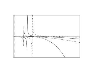
 $0 < \theta < 90^{\circ }$). This result is manifested clearly in figures 2(a,b), which display the variation of
  $Re_c$ against
  $M$ for two distinct values of
  $E$ (
$E$ ( $=1$ and
  $3$) when
  $\theta =30^{\circ }$ and
  $75^{\circ }$, respectively. From these figures, it is easy to say that the realistic (positive) value
  $Re_c$ will exist up to the value
  $M \approx 4.62924$. However, this value
  $M \approx 4.62924$ is practically very large for thin film flow problems since most of the common liquids are poorly conducting. Thus to obtain the numerical results of this problem, we will consider (generally) the value of
  $M$, without loss of generality, in the range
  $0 \le M \le 1$ for the ranges
  $0 \le E \le 3$,
  $0< Re \le 100$ and
  $0<\theta \le 90^{\circ }$. Here, we will consider a fixed value
  $We =450$ as it is very large for practical applications.

Figure 2. Variation of  $Re_c$ with
  $M$ for some values of
  $E$ when (a)
  $\theta =30^{\circ }$ and (b)
  $\theta =75^{\circ }$. For
  $\theta =90^{\circ }$, the value of
  $Re_c$ is always zero whatever the values of
  $E$ and
  $M$ (see (4.15)).
A noteworthy result that can be found from figures 2(a,b) is that for a given value of  $\theta$ (
 $< 90^{\circ }$) and up to the value
  $E \approx 2.45$, the value of
  $Re_c$ increases continuously with the increase of
  $M$, while for a large value of
  $E$ (above the value
  $E \approx 2.45$), first the value of
  $Re_c$ decreases up to a certain minimum (dependent on
  $E$ and
  $\theta$) at a certain value of
  $M$ (e.g.
  $M_m$, independent of
  $\theta$), and then it increases and finally reaches infinity (a very large positive value of
  $Re_c$ depending upon the values of
  $E$ and
  $\theta$) owing to the fulfilment of the singularity condition of
  $Re_c$ at
  $M \approx 4.62924$. Hence we can conclude that the magnetic field will show the stabilizing influence on this flow field up to the value
  $E \approx 2.45$ independent of
  $\theta$, and after that value it follows (slowly) the destabilizing role but up to the value of
  $M_m$, and then continuously follows the stabilizing effect on this flow field. Another remarkable observation that can also be found from these figures is that for a smaller value of
  $E$ (or
  $\theta$), the (positive) value of
  $Re_c$ is always higher than for a larger value of
  $E$ (or
  $\theta$), and this result is more pronounced for a higher value of
  $M$, confirming the destabilizing influence of
  $E$ and
  $\theta$ on this flow field. Here, for
  $E =3$ and for both values
  $\theta =30^{\circ }$ and
  $75^{\circ }$, we have found the value
  $M_m \approx 0.73635$, which will increase for an increasing value of
  $E$ since it has a destabilizing influence on this flow field.
The magnetic field reduces (depresses) the steady basic flow velocity owing to the formation of the Lorentz resistive force by the interaction of the fluid velocity and the magnetic field inside the flow layer. By contrast, the Lorentz force, which is produced by the electric field (in the presence of a magnetic field), assists the downstream flow, resulting in the enhancement (uplifting) of the basic flow (see (2.11)). Indeed, the depression of the flow velocity causes the increase in the normal pressure on the plate surface, which essentially increases the attachment of the flow to the surface. In the sequel, the frictional force of the adjacent layer to the plate surface increases. Besides this, the deviation of the mean flow due to the perturbation is suppressed by the magnetic field as the magnetic line of force acts like an elastic string. The combined influence of these two forces stabilizes the liquid film flowing down an inclined plane in the presence of a magnetic field. An opposite explanation holds true for the application of an electric field (in the presence of a magnetic field) in the thin film flow problems. The opposite effects of electric and magnetic field go into competition inside the film flow layers, and ultimately, a mutually stable position originates in between the values of  $E$ and
  $M$, depending upon the values of
  $\theta$. In this stable position, the critical value
  $Re_c$ will be the same for both magnetic and non-magnetic cases. Here, we denote the values of
  $E$ and
  $M$ corresponding to the mutually stable position as
  $E_m$ and
  $M_e$. The value of
  $E_m$ is independent of
  $\theta$ but depends highly on the values of
  $M$. Obviously, the value of
  $E_m$ will be increased with an increasing value of
  $M$ owing to maintaining this mutually stable position, which one can perceive from figures 3(a,b). A comparative study of these two figures reveals that the value of
  $Re_c$ is always lower for a higher value of
  $\theta$, irrespective of the values of
  $E$ and
  $M$, confirming the destabilizing influence of
  $\theta$ on this flow field.

Figure 3. Variation of  $Re_c$ with
  $E$ for several values of
  $M$ when (a)
  $\theta =30^{\circ }$ and (b)
  $\theta =75^{\circ }$.

Figure 4.  $Re_c$ versus
  $\theta$ for some values of (a)
  $M$ when
  $E =0$, and (b)
  $E$ when
  $M =1$.

Figure 5. Variation of  $k_c$ against
  $Re$ for four distinct
  $M$ values at (a)
  $\theta =15^{\circ }$ and (b)
  $\theta =75^{\circ }$, when
  $E =0$. For
  $\theta =90^{\circ }$, the value of
  $k_c$ is maximum and independent of
  $Re$, and we have found
  $k_c =0.08161$,
  $0.06764$,
  $0.05470$ and
  $0.04203$ for
  $M =0.001$,
  $0.50$,
  $0.75$ and
  $1.0$, respectively.

Figure 6. Variation of  $k_c$ against
  $Re$ for four distinct
  $E$ values at (a)
  $\theta =15^{\circ }$ and (b)
  $\theta =75^{\circ }$, when
  $M =1$. For
  $\theta =90^{\circ }$, the value of
  $k_c$ is maximum and independent of
  $Re$, and we have found
  $k_c =0.04203$,
  $0.05604$,
  $0.07005$ and
  $0.08406$ for
  $E =0$,
  $1$,
$1$,  $2$ and
  $3$, respectively (see (4.14)).

Figure 7. Variation of  $k_c$ against
  $\theta$ for two distinct values of
  $Re$ (
 $=1$ and
  $10$), and for several values of (a)
  $E$ when
  $M =1$, and (b)
  $M$ when
  $E =0$.
In order to illuminate the above results more clearly, we depict the variation of  $Re_c$ against
  $\theta$ for several values of
  $M$ and
  $E$ in figures 4(a,b), respectively. It is well known that for the non-magnetic case (i.e. for
  $M =0$), the value of
  $Re_c$ decreases continuously with the increase of
  $\theta$, and ultimately vanishes at
  $\theta =90^{\circ }$ (see figure 3 of Dholey & Gorai Reference Dholey and Gorai2021). Here, both the parameters
  $E$ and
  $M$ follow the above trend but in opposite styles. For any given value of
  $\theta$ (
 $0<\theta <90^{\circ }$), the value of
  $Re_c$ decreases (or increases) continuously with the increase of
  $E$ (or
  $M$), confirming the destabilizing (or stabilizing) influence of
  $E$ (or
  $M$) on this flow field. Besides this, the decreasing (or increasing) rate of
  $Re_c$ with
  $E$ (or
  $M$) is always higher for a lower value of
  $\theta$, which confirms the destabilizing effect of
  $\theta$ in the presence of magnetic as well as electromagnetic fields.
The variation of  $k_c$ against
  $Re$ for four distinct values of
  $M$ (
$M$ ( $=0.001$,
  $0.50$,
  $0.75$ and
  $1$) is delineated in figures 5(a,b), corresponding to two fixed values,
  $\theta =15^{\circ }$ and
  $75^{\circ }$, respectively. Here, we have considered two representative values of
  $\theta$ (
 $=15^{\circ }$ and
  $75^{\circ }$) from which one can estimate easily the effect of the other values of
  $\theta$ on
  $k_c$ as well as on
  $Re_c$, especially on the stable and unstable zones in the
  $Re$–
$Re$– $k_c$ plane, except for
  $\theta =90^{\circ }$, for which
  $Re_c =0$ irrespective of the values of
  $E$ and
  $M$, and
  $k_c$ is independent of
  $Re$ but depends highly on the values of
  $E$ and
  $M$ (see (4.14) and (4.15)). For a given value of
  $\theta$ and for an increasing value of
  $M$, the critical value
  $k_c$ decreases while
  $Re_c$ increases, resulting in the increase of the linear stable zone, which ensures the stabilizing influence of
  $M$ on this flow field. The opposite impacts have been found for an increasing value of
  $E$, which can be observed readily from figures 6(a,b). A closer scrutiny at these figures reveals that for given values of
  $E$ and
  $M$, and for an increasing value of
  $\theta$, the critical value
  $k_c$ (and hence the linear unstable zone) increases with a concomitant decrease of
  $Re_c$. This result ensures that the value of
  $Re_c$ will be least (zero), and the value of
  $k_c$ (and hence the linear unstable zone) will be maximum, at
  $\theta =90^{\circ }$, depending upon the values of
  $E$ and
  $M$ (see figures 11 and 13). The physical reason behind such behaviour of the flow is the direct involvement of
  $\cot \theta$ (with a negative sign) in the expression for
  $k_c$.
Focusing on the fact that the maximum value of  $k_c$ occurs at
  $\theta =90^{\circ }$ independent of
  $Re$ and dependent on the values of
  $E$ and
  $M$, we plot the variation of
  $k_c$ against
  $\theta$ for two distinct values of
  $Re$ (
 $=1$ and
  $10$), and for some values of
  $E$ and
  $M$, in figures 7(a) and 7(b), respectively. Here, the critical value
  $k_c$ increases continuously with the increase of
  $\theta$ after reaching the bifurcation point
  $(\theta _c, 0)$, dependent on the values of
  $E$,
$E$,  $M$ and
  $Re$, and attains its maximum value at
  $\theta =90^{\circ }$. To maintain the mutually stable position, an increased value of
  $M$ increases the value of
  $\theta _c$ along with the decrease of
  $k_c$ resulting in the increase of the linear stable zone. An opposite result has been found for an increasing value of
  $E$ as well as
  $Re$. Finally, we can conclude that the maximum linear unstable zone in the
  $Re$–
$Re$– $k$ plane, as well as the
  $M$–
$M$– $k$ and
  $E$–
$E$– $k$ planes, will be occurring at the value
  $\theta =90^{\circ }$, dependent on the values of
  $E$ and
  $M$, as the cut-off wavenumber
  $k_c$ is the maximum thereat (see figures 8a and 9a).

Figure 8. The  $M$–
$M$– $k_c$ neutral curves for some values of (a)
  $Re$ and
  $\theta$ when
  $E =0$, and (b)
  $E$ and
  $Re$ when
  $\theta =45^{\circ }$. The curve for
  $\theta =90^{\circ }$ is independent of
  $Re$. Here, we have considered the values of
  $\theta$ that are greater than
  $\theta _c \approx 5.71597^{\circ }$,
  $18.45127^{\circ }$ and
  $26.58679^{\circ }$ for
  $Re =10$,
  $3$ and
  $2$, respectively.

Figure 9. The  $E$–
$E$– $k_c$ neutral curves for some values of (a)
  $\theta$ when
  $M =1$, and (b)
  $M$ when
  $\theta =15^{\circ }$, with a fixed value
  $Re =10$. Here, we are not presenting the curves
  $k_c$ for
  $\theta =0.2^{\circ }$,
  $0.5^{\circ }$,
  $1^{\circ }$,
  $2^{\circ }$ and
  $5^{\circ }$ for which we have found
  $E_c =28.19171$,
  $16.72716$,
  $10.94868$,
  $6.86170$ and
  $3.23043$, respectively.
For  $M\rightarrow 0$ (i.e. for
  $M =0.001$),
  $k_c$ has a fixed value, dependent on
  $Re$ and
  $\theta$ but independent of
  $E$, which decreases continuously with the increase of
  $M$, and ultimately vanishes at a definite value of
  $M$, for example,
  $M_c$ depending upon the values of
  $E$,
$E$,  $Re$ and
  $\theta$. Indeed, it is the critical value of
  $M$ below which the film flow is unstable, and beyond that value the flow will be stable. The above results are manifested clearly in figures 8(a,b).
Figure 8(a) displays the variation of  $k_c$ against
  $M$ for three different values of
  $\theta$ (
 $= 30^{\circ }$,
  $60^{\circ }$ and
  $90^{\circ }$) corresponding to two fixed values of
  $Re$ (
 $= 2$ and
  $3$) when
  $E =0$. For a given value of
  $\theta$ (
 $<90^{\circ }$) and for an increasing value of
  $Re$, the unstable zone increases along with the increase of
  $k_c$ and
  $M_c$ owing to its destabilizing impact on this flow field. The unstable zone also increases with the increase of
  $\theta$, and finally covers the most unstable zone in
  $\theta =90^{\circ }$ independent of the values of
  $Re$ (see also figure 17b). For
  $\theta =90^{\circ }$,
  $k_c$ is independent of
  $Re$ but relies on the values of
  $E$,
$E$,  $M$ and
  $We$ (see figures 11 and 13, and (4.14)). Besides this, the term within the second curly braces of (4.14) is zero for
  $M \approx 4.62924$, independent of the values of
  $E$ and
  $We$ (see also figure 2). Hence we see that for a vertical plane (i.e. for
  $\theta =90^{\circ }$), the value of
  $k_c$ will be zero at
  $M \approx 4.62924$, which is manifested clearly in figure 8(a). We have found earlier that the electric field is active only in the presence of a magnetic field. Hence we can conclude that the most unstable zone that occurs in
  $\theta =90^{\circ }$ will be increased (or decreased) with an increasing value of
  $E$ (or
  $We$) without changing the values of
  $k_c$ (non-magnetic) and
  $M_c$, as the parameter
  $E$ (or
  $We$) has a destabilizing (or stabilizing) effect on this flow field.
On the other hand, for given values of  $Re$ and
  $\theta$ (
 $<90^{\circ }$), and for an increasing value of
  $E$, the unstable zone increases with a concomitant increase of
  $M_c$, dependent on
  $Re$ and
  $\theta$, but without changing the initial (non-magnetic) values of
  $k_c$ (which depend on the values of
  $Re$ and
  $\theta$), as the electric field effect is zero in the non-magnetic case. These results are manifested clearly in figure 8(b). From figures 8(a,b), it is clear that the value of
  $M_c$ increases with the increase of
  $E$ as well as
  $Re$ and
  $\theta$ owing to their destabilizing influence on this flow field. Here, the stabilizing influence of
  $M$ balances (neutralizes) the destabilizing influence of the other parameters (
 $E$,
$E$,  $Re$ and
  $\theta$) separately or jointly, and therefore, for an increasing value of any one of the destabilizing parameters, the value of
  $M_c$ increases. Finally, we conclude that in the presence of an electric field, the magnetic field effect prevails in the competition (means provide only the stable zone) only for a value greater than
  $M_c$, while
  $M_c$ depends on the values of
  $Re$ and
  $\theta$.
From the foregoing analysis, it is clear that for the given values of any three of the parameters  $E$,
$E$,  $M$,
$M$,  $Re$ and
  $\theta$, the other parameter would have a critical value. Indeed, these are the four mutually critical values in the system for which the total stabilizing and destabilizing influences are balancing each other. To be more precise, a given value of a parameter, whatever may be its effect (stabilizing or destabilizing), and an increasing value of a parameter that has a stabilizing (or destabilizing) influence, essentially increases (or decreases) the parameter, which has a destabilizing influence for adjusting the total stabilizing and destabilizing influences on this flow field. In order to clarify this result, we show the variation of
  $k_c$ with
  $E$ for several values of
  $\theta$ and
  $M$ in figures 9(a) and 9(b), respectively.
For an increasing value of  $\theta$, the critical value
  $E_c$ decreases continuously, and it becomes zero after a definite value of
  $\theta$, for example
  $\theta _0$, that is dependent on
  $M$ and
  $Re$; after this value
  $\theta _0$, the value of
  $E_c$ will be negative, which one can guess easily from figure 9(a). Here, for
  $M =1$ and
  $Re =10$, the value of
  $\theta _0$ is obtained as
  $\theta _0 \approx 20.6740316^{\circ }$. Besides this, the value of
  $k_c$ increases with the increase of
  $\theta$ as well as
  $E$ owing to their destabilizing effect on this flow field. As a result, the unstable zone in the
  $E$–
$E$– $k$ plane increases with the increase of
  $\theta$, and finally it becomes maximum in
  $\theta =90^{\circ }$. An increased value of
  $\theta$ strengthens the destabilizing influence of the film flow, which essentially decreases the destabilizing influence of
  $E$ (the value of
  $E_c$) for balancing the mutually stable condition owing to the fixed values of other parameters
  $M$ (
$M$ ( $=1$) and
  $Re$ (
 $=10$). Similar results can also be found for an increasing value of
  $Re$ without changing the values of
  $M$ and
  $\theta$ since the parameter
  $Re$ has the same (destabilizing) influence found in the parameter
  $E$. And obviously, the opposite phenomenon has been found for an increasing value of
  $M$, which is manifested clearly in figure 9(b). Here, for
  $\theta =15^{\circ }$ and
  $Re =10$, the value of
  $M_0$ is obtained as
  $M_0 \approx 0.84205415$, for which
  $E_c =0$. From the above analysis, we come to the conclusion that the linear stable as well as unstable (and hence the range of all four distinct flow) zone(s) of this problem can be controlled easily by adjusting by a suitable amount the parameters
  $E$,
$E$,  $M$,
$M$,  $Re$ and
  $\theta$.
Dandapat & Mukhopadhyay (Reference Dandapat and Mukhopadhyay2003) examined the stability of a conducting liquid film flowing down an inclined plane in the presence of an electromagnetic field. They have analysed this problem only for the fixed values  $Re =10$ and
  $\theta =75^{\circ }$, and reported that the magnetic field stabilizes the film flow but not for too large values of
  $E$. However, the present analysis confirms that the value of
  $E_c$ is very sensitive (large) especially for the small values of
  $Re$ and
  $\theta$ in combination with a large value of
  $M$, which one can perceive easily from figures 9(a,b) (see also the figure's caption). Hence their result may be true for some particular values of
  $Re$ and
  $\theta$, but not in general, which we have claimed in this paper.
4.2. Results and discussion for weakly nonlinear stability analysis
Lin (Reference Lin1974) investigated the finite-amplitude side-band stability of a viscous film flowing steadily down an inclined plane where he stated that in the neighbourhood of the upper branch of the neutral curve  $k = k_c$, a thin band of width
  $\varsigma$ (
 $\ll 1$) of unstable mode develops over a time
  $O(\varsigma ^{-2})$ and over a distance
  $O(\varsigma )$ such that
  $\omega _i^+\sim O(\varsigma ^2)$. This phenomenon ensures that in the marginal state (
 $\omega _i^+ = 0$), all modes of the perturbation are neither stable nor unstable, which implies that the linear stability analysis can no longer predict the ultimate behaviour of the flow, therefore the nonlinear stability analysis is necessary for understanding the proper characteristics of the thin film flow down an inclined plane.
Weakly nonlinear stability analysis allows one to examine whether the nonlinear finite-amplitude disturbance in a linear stable zone creates instability (subcritical instability), and the nonlinear evolution of the disturbance decelerates the growth of linear disturbance for which a finite amplitude stable state may arise (supercritical stability), or it accelerates the growth of the linear disturbance, which causes an explosion. Here, we have used the multiple scale method for deriving the complex Ginzburg–Landau type equation (4.5), from which one can characterize easily the proper behaviour of the flow. In order to do this, we consider two sets of mutually independent variables,  $(x_1, x_2, \ldots )$ and
  $(t_1, t_2, \ldots )$, which are
 \begin{equation} x_1 = \varsigma x, x_2 = \varsigma^2 x,\ldots\quad \text{and} \quad t_1 = \varsigma t, t_2 = \varsigma^2 t,\ldots, \end{equation}
where  $\varsigma$ (
 $\ll 1$) provides the smallness of the corresponding variables. Here,
  $(x, t)$ are fast scales, while
  $(x_1, t_1)$, and so on, are slow scales. The temporal and spatial derivatives are obtained as
 \begin{equation} \partial_t \equiv \partial_t + \varsigma\,\partial_{t_1} + \varsigma^2\, \partial_{t_2} +\cdots\quad \text{and} \quad \partial_x \equiv \partial_x + \varsigma\,\partial_{x_1} +\cdots. \end{equation}
Here, we consider the asymptotic form of the surface elevation  $\eta (x, t)$ as
 \begin{equation} \eta(\varsigma, x, x_1, x_2,\ldots, t, t_1, t_2,\ldots) = \varsigma \eta_1 + \varsigma^2 \eta_2 + \varsigma^3 \eta_3 + \cdots.\end{equation}
Using (4.16a–c)–(4.18) in (4.5), we get
 \begin{equation} (L_0 + \varsigma L_1 + \varsigma^2 L_2 + \cdots)(\varsigma \eta_1 + \varsigma^2 \eta_2 + \varsigma^3 \eta_3 + \cdots) =- \varsigma^2 N_2 - \varsigma^3 N_3 - \cdots, \end{equation}
where  $L_0,L_1,L_2,\ldots$ are the operators, and
  $N_2,N_3,\ldots$ are the nonlinear terms of (4.19), which are given in Appendix A. From (4.19), one can obtain the lowest-order equation of
  $\varsigma$ as
 \begin{equation} L_0 \eta_1 = 0, \end{equation}
which has a solution of the form
 \begin{equation} \eta_1 = \varLambda (x_1, t_1, t_2) \exp \{ {\rm i}\varTheta \} + {\rm c.c.} , \end{equation}
where  $\varTheta =kx -\omega _r t$, and c.c. denotes the complex conjugates. The dispersion relation
  $D(\omega _r, k)$ of (4.21) will be the same as (4.8), except that
  $\omega$ would be
  $\omega _r$ since in the neighbourhood of
  $k =k_c$,
  $\omega _i^+ \sim O(\varsigma ^2)$, for which
  $\exp (\omega _i^+ t)$ is slowly varying and may be assimilated in
  $\varLambda (x_1, t_1, t_2)$.
From (4.19), the second-order equation of  $\varsigma$ is obtained as
 \begin{equation} L_0 \eta_2 =- L_1 \eta_1 - N_2. \end{equation}
Using (4.21) in (4.22), we get
 \begin{equation} L_0\eta_2 =- {\rm i} \left[ \frac{\partial D(\omega_r, k)} {\partial \omega_r}\,\frac{\partial \varLambda}{\partial t_1} - \frac{\partial D(\omega_r, k)} {\partial k}\,\frac{\partial \varLambda} {\partial x_1} \right]\exp \{ {\rm i} \varTheta \} - Q \varLambda^2 \exp \{ 2{\rm i} \varTheta \} + {\rm c.c.} ,\end{equation}
where  $Q =\textrm {i} (a_6 k - a_7\omega _r) - 2 a_8 \omega ^2_r - 2 a_9 k^2 + 2 a_{10} k^4$. From (4.23), the uniform valid solution for
  $\eta _2$ is given by
 \begin{equation} \eta_2 = Q_1 \varLambda^2 \exp\{2i\varTheta\} + {\rm c.c.}, \end{equation}
where  $Q_1= - Q/D(2 \omega _r, 2k)$. Introducing the coordinate transformations
  $\xi =(x_1 - c_g t_1)$ and
  $\tau =t_2$, where
  $c_g$ (
 $= -D_k/D_{\omega _r}$) is the group velocity in the
  $x$-direction, and using the solvability condition in the third-order equation of
  $\varsigma$, we have
 \begin{equation} \frac{\partial \varLambda}{\partial \tau} - \frac{{\rm i}}{2}\,c_g^{\prime}(k)\,\frac{\partial^2 \varLambda} {\partial \xi^2} - \varsigma^{-2} (F_r + i F_i) \omega_i \varLambda + (J_2 + {\rm i} J_4)\,|\varLambda|^2 \varLambda = 0, \end{equation}
which is the complex Ginzburg–Landau type equation. For  $M\rightarrow 0$, (4.25) corroborates (49) of Dholey & Gorai (Reference Dholey and Gorai2021) as the values of the coefficients
  $c_g^{\prime }$,
  $F_r$,
  $F_i$,
  $J_2$ and
  $J_4$ (which are given in Appendix B) reduce to the same as presented in (50) of Dholey & Gorai (Reference Dholey and Gorai2021).
For a filtered wave,
 \begin{equation} \frac{\partial \varLambda}{\partial \tau} - \varsigma^{-2} (F_r + {\rm i} F_i) \omega_i \varLambda + (J_2 + {\rm i} J_4)\,|\varLambda|^2 \varLambda = 0. \end{equation}
The solution of (4.26) may be written as
 \begin{equation} \varLambda = a\exp [- {\rm i} b(\tau)\,\tau], \end{equation}
which on substitution in (4.26), and then equating the real and imaginary parts, gives
 \begin{equation} \frac{\partial a}{\partial \tau} = \big(\varsigma^{-2} F_r \omega_i - J_2 a^2 \big)a \end{equation}
and
 \begin{equation} \frac{\partial \{b(\tau)\,\tau \} }{\partial \tau} = \big( J_4 a^2 - \varsigma^{-2} F_i \omega_i \big). \end{equation}
The sign of  $J_2$ (second Landau constant) that appears in (4.28) due to nonlinearity in the system plays a significant role in determining the varied flow zones of this problem. A positive value of
  $J_2$ ensures the saturation of the amplitude of the disturbance, which essentially helps one to delimit the supercritical stability in the linear unstable zone
  $(\omega _i^+ > 0)$ and the unconditional stability in the linear stable zone (
 $\omega _i^+<0$). By contrast, saturation of the amplitude does not occur in a negative value of
  $J_2$, which helps one to demarcate the explosive state in the linear unstable zone (
 $\omega _i^+ > 0$) and the subcritical instability in the linear stable zone (
 $\omega _i^+<0$).
The perturbed wave speed induced by the infinitesimal disturbances appearing in the nonlinear system can be modified by using (4.29). Finally, the threshold amplitude and nonlinear phase velocity are given by
 \begin{equation} \varsigma a = \left( F_r \omega_i/J_2 \right)^{1/2} \end{equation}
and
 \begin{equation} Nc_{r} = c_r + c_i (J_4 F_r/J_2 - F_i), \quad \text{where} \ c_i = \omega_i/k. \end{equation}
 Mukhopadhyay et al. (Reference Mukhopadhyay, Dandapat and Mukhopadhyay2008) investigated the influence of an electromagnetic field on the stability of a conducting liquid film flowing down an inclined plane, where they have demarcated four different flow zones of this problem under various values of  $E$ and
  $M$ when
  $\theta =75^{\circ }$ (see figures 3–9 there). However, the demarcations of four different flow zones that are found in their paper are not correct for the following reason. It is noticeable that the curve
  $J_2$ (
 $E$,
$E$,  $k$,
$k$,  $M$,
$M$,  $Re$,
$Re$,  $We$,
$We$,  $\theta$), which will be obtained from the relations as given in (B1), has a singular point only when the relationship (singularity condition)
 $$\begin{gather} \left [ \frac{a_0}{M^2} \left(1 - \frac{\tanh M}{M}\right) \right ]^2 \Bigg [ \left(1 + \frac{2\tanh M}{M}\right)^2 - \alpha \left(1 + \frac{4\tanh M}{M} \right) \Bigg] Re \nonumber\\ {}- 3 \cot\theta - 4 Re\,We\,k^2 = 0 \end{gather}$$
is fulfilled. For given values of any five of the parameters  $E$,
$E$,  $k$,
$k$,  $M$,
$M$,  $Re$,
$Re$,  $We$ and
  $\theta$, (4.32) gives the value of the other at which a singularity of
  $J_2$ occurs. For example, if one deals with the values
  $E =0$,
  $M =0.001$ (i.e.
  $M\rightarrow 0$),
  $Re =100$,
  $We =450$ and
  $\theta =45^{\circ }$, then one gets
  $k_s \approx 0.04060$, which completely agrees with the result represented in figure 19(b). From this figure it is clear that below the value of
  $k_s$, the curve
  $J_2$ is always negative. Besides this, a close relationship between
  $k_s$ and
  $k_c$ is obtained from (4.32) and (4.14) as
 $$\begin{gather} k_s = \frac{1}{2}
\sqrt{ \frac{\left\{ \dfrac{a_0}{M^2} \left(1 -
\dfrac{\tanh M}{M}\right) \right\}^2 \Bigg\{ \left(1 +
\dfrac{2\tanh M}{M}\right)^2 - \alpha \left(1 +
\dfrac{4\tanh M}{M} \right) \Bigg\}Re - 3 \cot\theta
}{Re\,We} }\nonumber\\ = \frac{k_c}{2},
\end{gather}$$
$$\begin{gather} k_s = \frac{1}{2}
\sqrt{ \frac{\left\{ \dfrac{a_0}{M^2} \left(1 -
\dfrac{\tanh M}{M}\right) \right\}^2 \Bigg\{ \left(1 +
\dfrac{2\tanh M}{M}\right)^2 - \alpha \left(1 +
\dfrac{4\tanh M}{M} \right) \Bigg\}Re - 3 \cot\theta
}{Re\,We} }\nonumber\\ = \frac{k_c}{2},
\end{gather}$$
which one can check easily from figure 19(a,b). Equation (4.33) ensures that the curve  $k_s$ separates the existing linear unstable zone (
 $\omega _i^+ > 0$) into two equal parts without changing the critical values of
  $Re_c$ or
  $\theta _c$ or
  $M_c$ or
  $E_c$. Hence the lower region of the curve
  $k_s$ is entirely an explosive zone as there
  $J_2$ is negative, while the upper region may be either wholly a supercritical zone or partly supercritical and partly an explosive zone. This depends on whether the curve
  $J_2 =0$ would not cross the curve
  $k_c$ or cross it (see figures 10–18). From the above analysis, it is confirmed that the graphical representation, especially the demarcations of four different flow zones of this problem presented by Mukhopadhyay et al. (Reference Mukhopadhyay, Dandapat and Mukhopadhyay2008), are not correct, therefore the results based on these figures have doubtful validity, as claimed earlier.

Figure 10. Neutral stability curves in the  $Re$–
$Re$– $k$ plane showing four different flow zones at four different values (a)
  $M =0.001$, (b)
  $M =0.25$, (c)
  $M =0.50$ and (d)
  $M =1.0$, when
  $E =0$,
  $We =450$ and
  $\theta =45^{\circ }$. The four different zones found in (a) agree well with the corresponding zones reported by Dholey & Gorai (Reference Dholey and Gorai2021) in figure 6 of their analysis. A small discrepancy is found in the values of
  $k$ and
  $Re_c$ owing to the consideration of
  $M =0.001$ instead of
  $M =0$.

Figure 11. Neutral stability curves in the  $Re$–
$Re$– $k$ plane showing four different flow zones at four different values (a)
  $M =0.001$, (b)
  $M =0.25$, (c)
  $M =0.50$ and (d)
  $M =1.0$, when
  $E =0$,
  $We =450$ and
  $\theta =90^{\circ }$. The four different zones found in (a) agree well with the corresponding zones reported by Dholey & Gorai (Reference Dholey and Gorai2021) in figure 13(d) of their analysis.

Figure 12. Neutral stability curves in the  $Re$–
$Re$– $k$ plane showing four different flow zones at two different values (a)
  $E =1$ and (b)
  $E =3$. The other parameters are chosen as
  $M =1$,
  $We =450$ and
  $\theta =45^{\circ }$. For
  $E =0$, the variation of the same flow zones can be found from figure 10(d).

Figure 13. Neutral stability curves in the  $Re$–
$Re$– $k$ plane showing four different flow zones at two different values (a)
  $E =1$ and (b)
  $E =3$. The other parameters are chosen as
  $M =1$,
  $We =450$ and
  $\theta =90^{\circ }$. For
  $E =0$, the variation of the same flow zones can be found from figure 11(d).

Figure 14. Neutral stability curves in the  $\theta$–
 $k$ plane showing four different flow zones at four different values (a)
  $M =0.001$, (b)
  $M =0.25$, (c)
  $M =0.50$ and (d)
  $M =1.0$, when
  $E =0$,
  $Re =10$ and
  $We =450$. The four different zones that are found in (a) agree well with the corresponding zones reported by Dholey & Gorai (Reference Dholey and Gorai2021) in figure 10(c) of their analysis.

Figure 15. Neutral stability curves in the  $\theta$–
 $k$ plane showing four different flow zones at two different values (a)
  $E =1$ and (b)
  $E =3$. The other parameters are chosen as
  $Re =10$,
  $M =1$ and
  $We =450$. For
  $E =0$, the variation of the same flow zones can be found from figure 14(d).

Figure 16. Neutral stability curves in the  $E$–
$E$– $k$ plane showing four different flow zones at two distinct values (a)
  $\theta =15^{\circ }$ and (b)
  $\theta =90^{\circ }$, when
  $M =1$,
  $Re =10$ and
  $We =450$.

Figure 17. Neutral stability curves in the  $M$–
$M$– $k$ plane showing four different flow zones at two different values (a)
  $\theta =75^{\circ }$ and (b)
  $\theta =90^{\circ }$, when
  $E =0$,
  $Re =10$ and
  $We =450$. We have found
  $M_c \approx 0.84205$ and
  $1.40676$ for
  $\theta =15^{\circ }$ and
  $45^{\circ }$, respectively.

Figure 18. Neutral stability curves in the  $M$–
$M$– $k$ plane showing four different flow zones at two different values (a)
  $E =1$ and (b)
  $E =2$, when
  $Re =10$,
  $We =450$ and
  $\theta =60^{\circ }$. We have found
  $M_c =1.62591$ and
  $3.90578$ for
  $E =0$ and
  $3$, respectively.

Figure 19. Variation of (a)  $\omega _i^+$ and (b)
  $J_2$ with
  $k$ for some values of
  $M$ when
  $E =0$,
  $Re =100$,
  $We =450$ and
  $\theta =45^{\circ }$. We have
  $k_j >k_c$,
  $k_j =k_c$ or
  $k_j < k_c$ accordingly as
  $M<0.68497$,
  $M=0.68497$ or
  $M>0.68497$.
Considering the relationship (4.33) as well as the signs of  $\omega _i^+$ and
  $J_2$, we have demarcated all the (correct) four distinct flow zones of this problem in figures 10–18 for the prescribed ranges of
  $E$,
$E$,  $M$ and
  $\theta$. Here, we have included the curves (figures) for
  $M =0.001$ (i.e. for
  $M\rightarrow 0$) only to validate the present (non-magnetic) results with the corresponding results reported by Dholey & Gorai (Reference Dholey and Gorai2021) (see figures 6, 10c and 13d there). In comparison, a negligible discrepancy is found owing to consideration of the value
  $M =0.001$ instead of
  $M =0$.
For the non-magnetic case (i.e. for  $M =0.001$) and for the given values
  $E =0$ and
  $\theta =45^{\circ }$, all four distinct zones in the
  $Re$–
$Re$– $k$ plane exist only after the critical value
  $Re_c$,and all the zones remain practically constant after a certain value of
  $Re$ as the curves
  $\omega _i^+ =0$ and
  $J_2 =0$ get their corresponding asymptotic nature after that value of
  $Re$ (see figure 10a). By contrast, for a given value of
  $M$ (not too small), the curve
  $J_2 =0$ does not follow the asymptotic behaviour with
  $Re$, and while following the same asymptotic behaviour, the curve
  $\omega _i^+ =0$ depresses gradually towards the
  $Re$-axis with a concomitant increase of
  $Re_c$ for which the unconditional stable zone increases (but up to the value
  $Re_c$) along with the decrease of the supercritical stable as well as the explosive unstable zone, which confirms the stabilizing effect of
  $M$ on this flow field. For a given value of
  $Re$, the curve
  $J_2 =0$ decreases continuously with the increase of
  $M$, resulting in the increase of the subcritical unstable zone. The above results are observed directly from figures 10(b–d). Here, in the presence of a magnetic field, the curve
  $J_2 =0$ decreases continuously with the increase of
  $Re$, and finally it crosses the curve
  $\omega _i^+ =0$ after a certain value
  $Re_0$ of
  $Re$, dependent on
  $M$, at which the stabilizing influence of
  $M$ dies out because of the destabilizing influence of
  $Re$ (see figure 10d). Hence we see that the unconditional stable zone of this flow problem will exist only up to the value
  $Re_0$, and beyond that value, a new explosive unstable zone will arise that increases with the increase of
  $Re$ owing to the destabilizing influence of
  $Re$ on this flow field. Finally, we come to the conclusion that in the presence of a magnetic field, all four distinct flow zones of this problem will exist in a definite range
  $(Re_c, Re_0)$ of
  $Re$, and the unconditional stable zone will vanish after the value
  $Re_0$ depending upon the values of
  $E$,
$E$,  $M$ and
  $\theta$.
The corresponding variations of the curves  $\omega _i^+ =0$ and
  $J_2 =0$ for a vertical plane (i.e. for
  $\theta =90^{\circ }$) are delineated in figures 11(a–d) with the same values of
  $E$,
$E$,  $M$ and
  $We$ as considered in figures 10(a–d). In this case, the curve
  $\omega _i^+ =0$ is free from
  $Re$, and the value of
  $Re_c$ is zero irrespective of the values of
  $E$ and
  $M$ (see (4.14) and (4.15)). By contrast, the curve
  $J_2 =0$ depends highly on the values of
  $Re$. Here, the parameters
  $M$ and
  $Re$, especially for the curve
  $J_2 =0$, follow the same behaviour as we have found in figures 10(a–d). A comparative study (of the corresponding parts) of figures 10 and 11 reveals that for an increasing value of
  $\theta$, the unconditional stable zone decreases along with the increase of the explosive unstable zone. An increased value of
  $\theta$ increases the destabilizing influence in the film flow dynamics, which essentially reduces the existing destabilizing influence of
  $Re$ for neutralizing the stabilizing influence of
  $M$ (which is now fixed at a given value), resulting in the decrease of the value of
  $Re_0$, the upper limit of
  $Re$ for the existence of four distinct flow zones of this problem.
Next, let us look at figures 12(a,b), which are depicted for the same values of  $M$,
$M$,  $We$ and
  $\theta$ as considered in figure 10(d), and convey the information about the range
  $(Re_c, Re_0)$ of
  $Re$ for four distinct flow zones of this problem for various values of
  $E$. An increased value of
  $E$ decreases the values of
  $Re_c$ and
  $Re_0$, indicated on the figures, along with the increase of the values of
  $k_c$ and
  $k_j$. Actually, an inclusion of
  $E$ enhances the destabilizing influence in the flow system, which is the essential cause of the decrease of
  $Re_c$ and
  $Re_0$ as well as the increase of
  $k_c$ and
  $k_j$. As a result, the unconditional stable zone decreases along with the increase of the explosive unstable zone. Besides this, the new explosive unstable zone arises after the value of
  $Re_0$ increases with the increase of
  $E$ owing to its destabilizing influence on this flow dynamics. Quite notably, if one increases the value of
  $\theta$ without changing the values of other parameters, then one gets more effective results than we have found from figures 12(a,b) (see figures 13a,b). When
  $E$ is added with
  $\theta$ (or
  $\theta$ is increased with a given value of
  $E$), they are united and act jointly on the flow system, and the resulting destabilizing influence makes the flow more unstable, which decreases the range
  $(Re_c, Re_0)$ of
  $Re$ for four distinct flow zones of this problem.
However, the new information that comes from figures 10–13 is that for an increasing value of  $M$, the unconditional stable zone increases up to the value
  $Re_c$, and then decreases and finally vanishes at the value
  $Re_0$, depending upon the values of
  $E$ and
  $\theta$. Hence, for the given values of
  $E$,
$E$,  $M$ and
  $\theta$, we can divide the whole
  $Re$ range into the following subintervals, from which one can easily recognize the number of different flow zones of this problem.
(i) For
 $0< Re \le Re_c$, two zones exist, namely subcritical unstable and unconditional stable. This result is true for all values of $\theta$ except $\theta =90^{\circ }$, for which $Re_c =0$.
(ii) For
$Re_c< Re< Re_0$, all four distinct zones of this flow problem are found for any given value of $\theta$ in $0<\theta \le 90^{\circ }$.(iii) For
$Re =Re_0$, all four zones, except the unconditional stable zone, of this flow problem exist for the full range of $\theta$ ($0<\theta \le 90^{\circ }$).(iv) For
$Re_0< Re \le 100$, the unconditional stable zone does not exist, while the existence of the other three zones is found for all values of $\theta$ considered in the present study. Here, a new explosive unstable zone (instead of an unconditional stable zone) originates after the value $Re_0$, which increases with the increase of $E$ as well as $Re$ and $\theta$.


We conclude our discussion by making some comments on the existence of four distinct flow zones of this problem under various values of the parameters  $E$,
$E$,  $M$,
$M$,  $Re$ and
  $\theta$. The relation
  $k_c =0$ yields not only the critical value
  $Re_c$ but also the critical value
  $E_c$, as well as
  $M_c$ and
  $\theta _c$. The critical value of any one of the parameters
  $E$,
$E$,  $M$,
$M$,  $Re$ and
  $\theta$ can be obtained by imposing the values of the other three parameters into the relation
  $k_c =0$, and these are the four mutually critical values of the system. Hence, for a given value of
  $Re$ in
  $(Re_c, Re_0)$, there is a critical value
  $\theta _c$, dependent on the values of
  $E$ and
  $M$, after which the linear instability arises in the flow system and one finds the existence of all four distinct flow zones of this problem (see condition (ii)). Similar results can also be found after the value
  $E_c$ since both the parameters
  $E$ and
  $\theta$ have the same (destabilizing) characteristic features on this flow dynamics. By contrast, all four distinct zones of this problem will be found up to the value
  $M_c$ since the magnetic field has a stabilizing influence on this flow field.
In order to clarify the above results, we have plotted the curves  $\omega _i^+ =0$ and
  $J_2 =0$ in the
  $\theta$–
 $k$,
$k$,  $E$–
$E$– $k$ and
  $M$–
$M$– $k$ planes for a fixed value
  $Re =10$, which obviously belongs to the range
  $Re_c< Re< Re_0$ for the ranges
  $0 \le E \le 3$,
  $0 \le M \le 1$ and
  $0<\theta \le 90^{\circ }$ (see figures 10–13), in figures 14–18. Figures 14(a–d), which are delineated for
  $E =0$, show that for a given value of
  $M$ and for an increasing value of
  $\theta$, the explosive unstable zone increases after reaching the critical value
  $\theta _c$, and simultaneously the unconditional stable zone decreases (slowly), confirming the destabilizing impact of
  $\theta$ on this flow dynamics. For an increasing value of
  $M$, the curves
  $\omega _i^+ =0$ and
  $J_2 =0$ depress towards the
  $\theta$-axis with a concomitant increase of
  $\theta _c$, resulting in the increase of the unconditional stable zone along with the decrease of the explosive unstable zone, which again confirms the stabilizing influence of the magnetic field on this flow problem. The opposite phenomena have been found for an increasing value of
  $E$, which one can perceive easily from figures 14(d) and 15(a,b). This is compatible with the fact that for an increasing value of
  $E$ as well as
  $\theta$, the destabilizing influence of the film flow is intensified, and simultaneously the stabilizing influence of
  $M$ (which is now fixed at a given value) becomes more and more feeble in comparison with the growing destabilizing influence of
  $E$ and
  $\theta$.
We have already shown in figure 9(a) that for  $M =1$ and
  $Re =10$, and for an increasing value of
  $\theta$, the value of
  $E_c$ decreases continuously and ultimately vanishes at the value
  $\theta _0 \approx 20.6740316^{\circ }$. This phenomenon ensures that for the same values of
  $M$ and
  $Re$, all four distinct zones of this flow problem will exist in the range
  $E_c< E \le 3$ or
  $0 \le E \le 3$ of
  $E$, accordingly as
  $\theta <\theta _0$ or
  $\theta >\theta _0$, as manifested clearly in figures 16(a) and 16(b), respectively. Here, for a given value of
  $\theta$, the increasing rate of the critical value
  $k_c$ (related to the curve
  $\omega _i^+ =0$) with
  $E$ is always higher than that of
  $k_j$ (related to the curve
  $J_2 =0$), resulting in the decrease of the unconditional stable and subcritical unstable zones, with a concomitant increase of the other two zones of this flow problem. This result is more pronounced for a higher value of
  $\theta$, which confirms our earlier results presented in figures 12, 13 and 15.
Each of figures 10, 11 and 14 ensures that for any given values of  $E$,
$E$,  $Re$ and
  $\theta$ within their prescribed ranges, the curves
  $\omega _i^+ =0$ and
  $J_2 =0$ decrease continuously with an increasing value of
  $M$. This fact confirms that the critical values of
  $k_c$ (related to the curve
  $\omega _i^+ =0$) and
  $k_j$ (related to the curve
  $J_2 =0$) will be zero separately after a definite (generally different) value of
  $M$, depending upon the values of
  $E$,
$E$,  $Re$ and
  $\theta$. For this reason, one finds the existence of two distinct critical values of
  $M$: one for
  $k_c =0$ denoted
  $M_c$, and the other for
  $k_j =0$ denoted
  $M_j$. Focusing on this fact, we plot the curves
  $\omega _i^+ =0$ and
  $J_2 =0$ in the
  $M$–
$M$– $k$ plane for two fixed values
  $\theta =75^{\circ }$ and
  $90^{\circ }$ when
  $E =0$ in figures 17(a,b), and for two fixed values
  $E =1$ and
  $2$ when
  $\theta =60^{\circ }$ in figures 18(a,b), respectively. A review of these figures discloses that the wavenumber
  $k_j$ is zero at
  $M_j \approx 3.99730$ irrespective of the values of
  $E$,
$E$,  $Re$ and
  $\theta$, confirming that the value of
  $M_j$ is constant for this problem. By contrast, the value of
  $M_c$ increases continuously with the increase of any one of the parameters
  $E$,
$E$,  $Re$ and
  $\theta$, owing to their destabilizing influence on this flow field. An increased value of
  $\theta$ (or
  $E$ or
  $Re$) increases the value of
  $k_c$, which in turn leads to an increase in the value of
  $M_c$ for vanishing this increased value of
  $k_c$ (see figures 10, 12 and 14–16). For
  $\theta =90^{\circ }$, the value of
  $\cot \theta$ is zero, and for
  $M \approx 4.62924$, the second curly braces term in the expression for
  $k_c$ is zero (see (4.14)). Hence for the values
  $\theta =90^{\circ }$ and
  $M \approx 4.62924$, the value of
  $k_c$ will be zero irrespective of the values of
  $E$ and
  $Re$, which is manifested clearly in figure 17(b), confirming our earlier result presented in figure 2.
Now we will explain graphically the reason for the existence of two distinct critical values of  $M$ in this problem. For this purpose, we depict the curves
  $\omega _i^+$ and
  $J_2$ against
  $k$ for some values of
  $M$ (
$M$ ( $=0.001$,
  $0.68497$ and
  $1.0$) in figures 19(a) and 19(b), respectively. For an increasing value of
  $M$, the values of
  $k_c$ and
  $k_j$ decrease along with the increase of the negative portions of the curves
  $\omega _i^+$ and
  $J_2$. More precisely, we can say that the values of
  $k_c$ and
  $k_j$ come close to zero, and the curves
  $\omega _i^+$ and
  $J_2$ depress towards their negative axes. This phenomenon suggests that the values of
  $k_c$ and
  $k_j$ will separately be zero (generally) for two distinct (but definite) values of
  $M$, ensuring the existence of two critical values of
  $M$ in this flow problem.
(i) One value of
$M$, for which $k_c =0$, is denoted by $M_c$, which depends highly on the values of $E$, $Re$ and $\theta$. Here, for the given values $E =0$, $Re =100$ and $\theta =45^{\circ }$, we have obtained $M_c \approx 2.33$, which one can easily and directly appreciate from figure 19(a). Interestingly enough, the curve $\omega _i^+$ will be wholly negative after the value of $M_c$, therefore there is no way for the occurrence of explosive unstable and supercritical stable zones of this flow problem (see figures 17 and 18).(ii) The other value of
$M$, for which $k_j =0$, is denoted by $M_j$, which is obtained as $M_j \approx 3.99730$, independent of the values of $E$, $Re$ and $\theta$ (see figure 19b). At the value $M_j$, the unconditional stable zone vanishes, and one finds only the existence of a subcritical unstable zone. After the value $M_j$, a new unconditional stable zone originates in the system that increases (slowly) with the increase of $M$ (see figures 17 and 18).


Dandapat & Mukhopadhyay (Reference Dandapat and Mukhopadhyay2003) examined the stability of a conducting liquid film flowing down an inclined plane in the presence of an electromagnetic field using the long-wave approximation method. They have shown the existence of two distinct critical values of  $M$, namely,
  $M_c$ and
  ${\bar M_c}$ in their figure 3, which is same as figure 17(a) of the present study. A comparative study between these two figures reveals that the characteristic features of the curve
  $\omega _i^+ =0$ with respect to
  $M$ are the same; nevertheless, a small discrepancy has been found in the values of
  $M_c$ due to the employment of different numerical methods. On the contrary, the features of the curve
  $J_2 =0$ that are found from figure 17(a) are completely different from those in figure 3 of Dandapat & Mukhopadhyay (Reference Dandapat and Mukhopadhyay2003). From their figure 3, it seems that they have considered the value
  ${\bar M_c} \approx 1.253$ for which the curve
  $J_2 =0$ has a point of discontinuity, which is doubtful. For clarity, we have checked many times the mathematical calculations and the numerical program for the expression of the curve
  $J_2 =0$, and finally obtained (tested) the results (numerically) for all values of
  $M$ (
$M$ ( $0 \le M \le 5$) in combination with the values of
  $E$,
$E$,  $Re$ and
  $\theta$ considered for this study. It is found that the curve
  $J_2 =0$ decreases continuously with the increase of
  $M$, and finally vanishes at
  $M_j \approx 3.99730$, independent of the values of
  $E$,
$E$,  $Re$ and
  $\theta$, which is shown in figures 17 and 18. Hence the curve
  $J_2 =0$ that was plotted by Dandapat & Mukhopadhyay (Reference Dandapat and Mukhopadhyay2003) in their figure 3 is not correct as claimed.
Finally, we conclude our discussion by stating the reason for the existence of the second range of  $k$ for an explosive unstable zone that occurs after the value of
  $Re_0$, depending upon the values of
  $E$,
$E$,  $M$,
$M$,  $We$ and
  $\theta$. Quite notably, this occurs only in the presence of a magnetic field. For
  $M =1$, two ranges of
  $k$ for the explosive unstable zone are found in figures 10–13. The first occurs only when the singularity condition (4.32) of
  $J_2$ is fulfilled. Equation (4.33) confirms the existence of a singularity of
  $J_2$ at the value
  $k =k_s$ (
 $=k_c/2$), below which
  $J_2$ is negative and
  $\omega _i^+$ is positive always, therefore
  $0< k< k_s$ is the range of
  $k$ for an explosive unstable zone generally found in the papers published by the authors concerned (see figures 5 and 12 of Dholey & Gorai Reference Dholey and Gorai2021).
An increased value of  $M$ decreases the values of
  $k_j$ and
  $k_c$ in which the decreasing rate of
  $k_j$ is higher than that of
  $k_c$ (see figures 19a,b). As a result, the value of
  $k_j$ crosses the value of
  $k_c$ after a certain value of
  $M$, dependent on
  $E$,
$E$,  $Re$ and
  $\theta$, which obviously follows the relationship
 \begin{equation} k_j \le k_c. \end{equation}
(i) When
$k_j =k_c$, we denote the parameters related to this case as the same parameters with a zero subscript. For example, if one considers figures 19(a,b), then one gets $k_j =k_c =0.05757$ for $E_0 =0$, $M_0 =0.68497$, $Re_0 =100$, $We_0 =450$ and $\theta _0 =45^{\circ }$. In this case, the unconditional stable zone vanishes, and one finds the existence of the other three zones of this problem.(ii) When
$k_j< k_c$, a new range $k_j< k< k_c$ of $k$ is found in which $J_2$ is negative and $\omega _i^+$ is positive always (see figures 19a,b). Indeed, it is the range of $k$ for an explosive unstable zone that newly arises (in place of unconditional stable zone) under a suitable value of $M$ depending upon the values of the other parameters.


Hence we can conclude that the condition for the existence of the number of the range of  $k$ for an explosive unstable zone is one or two accordingly as
  $k_j>k_c$ or
  $k_j< k_c$, and for the non-existence of an unconditional stable zone, the condition is
  $k_j \le k_c$. Most importantly, the first condition (
 $k_j> k_c$) occurs in both magnetic and non-magnetic cases, while the other two conditions (
 $k_j \le k_c$) occur only in the presence of a magnetic field.
5. Conclusion
We have examined in detail the effect of a magnetic as well as an electromagnetic field on the linear and weakly nonlinear stability of an electrically conducting viscous fluid film flowing down an inclined plane by assuming the magnetic Reynolds number to be small. A normal mode technique and multiple-scale method have been used to derive the results of linear and nonlinear stability analysis of this problem, respectively. Both results confirm the stabilizing influence of  $M$ and
  $We$, and the destabilizing influence of
  $E$,
$E$,  $Re$ and
  $\theta$ on this flow dynamics as well. A new feature that emerges from this analysis is the separation of all four distinct (explosive, supercritical, unconditional and subcritical) flow zones in the
  $Re$–
$Re$– $k$,
$k$,  $\theta$–
 $k$,
$k$,  $M$–
$M$– $k$ and
  $E$–
$E$– $k$ planes, from which one can easily recognize the proper zone of this flow problem under any given values of
  $E$,
$E$,  $k$,
$k$,  $M$,
$M$,  $Re$ and
  $\theta$. However, all four distinct flow zones of this problem exist prior to (or next to) the critical value of a stabilized (or destabilized) parameter provided that the curve
  $J_2 =0$ does not cross the curve
  $\omega _i^+ =0$. Especially in the
  $Re$–
$Re$– $k$ plane, for a suitable value of
  $M$, dependent on
  $E$ and
  $\theta$, the curve
  $J_2 =0$ crosses the curve
  $\omega _i^+ =0$ for which the unconditional stable zone vanishes at the crossing point
  $(Re_0, k_0)$. And after the value
  $Re_0$, a new (second) explosive unstable zone originates in the flow system, which increases with the increase of
  $Re$ as well as
  $E$ and
  $\theta$. The new information that comes from this analysis is the conditions for the non-existence of an unconditional stable zone, as well as the existence of one or two numbers in the range of
  $k$ for an explosive unstable zone, which are essentially the relations between
  $k_c$ and
  $k_j$ that depend highly on the values of
  $M$. Besides this, the existence of two critical values of
  $M$ are found: one is
  $M_c$, which depends on the values of
  $E$,
$E$,  $Re$ and
  $\theta$, while the other is constant, which is
  $M_j \approx 3.99730$. Finally, we conclude that the destabilizing influence of an electric (or Reynolds number or angle of inclination) parameter on this flow field can be controlled by applying a suitable amount of a magnetic (stabilizing) parameter, depending upon the values of the other parameters related to the problem.
Acknowledgements
We would like to thank the editors and reviewers for their useful comments that helped to improve the quality of the paper. Thanks are also due to Dr J. Dangar, S. Dholey and A. Dholey for their kind cooperation during the work.
Declaration of interests
The authors report no conflict of interest.
Appendix A
Expressions for  $L_0, L_1, L_2$ and
  $N_2, N_3$ are
 \begin{equation} \left. \begin{aligned} L_0 & \equiv \partial_t + a_1 \partial_x + a_2 \partial^2_{t} + a_3\partial_{x} \partial_{t} + a_4 \partial^2_{x} + a_5 \partial^4_{x} ,\\ L_1 & \equiv \partial_{t_1} + a_1 \partial_{x_1} + 2 a_2 \partial_{t} \partial_{t_1} + a_3 (\partial_{x} \partial_{t_1} + \partial_{x_1} \partial_{t}) + 2 a_4 \partial_{x} \partial_{x_1} + 4 a_5 \partial^3_{x} \partial_{x_1} ,\\ L_2 & \equiv \partial_{t_2} + a_2 ( \partial^2_{t_1} + 2 \partial_{t} \partial_{t_2} ) + a_3 (\partial_{x} \partial_{t_2} + \partial_{x_1} \partial_{t_1} ) + a_4 \partial^2_{x_1} + 6 a_5 \partial^2_{x} \partial^2_{x_1} , \\ N_2 & = a_6 (\eta_1 \eta_{1x}) + a_7( \eta_1 \eta_{1t}) + a_8( \eta_1 \eta_{1t})_t + a_9 (\eta_1 \eta_{1x})_x + a_{10} (\eta_1 \eta_{1xxx})_x ,\\ N_3 & = a_6 ( \eta_1 \eta_{1 x_1} + \eta_1 \eta_{2 x} + \eta_2 \eta_{1 x} ) + a_7 (\eta_1 \eta_{1 t_1} + \eta_1 \eta_{2 t} + \eta_2 \eta_{1 t} )\\ & \quad + a_8 \left \{ (\eta_1 \eta_{1 t_1} + \eta_1 \eta_{2 t} + \eta_2 \eta_{1 t} )_t + (\eta_1 \eta_{1 t})_{t_1} \right\} \\ & \quad + a_9 \left\{ ( \eta_1 \eta_{1 x_1} + \eta_1 \eta_{2 x} + \eta_2 \eta_{1 x} )_x + (\eta_1 \eta_{1 x})_{x_1} \right\}\\ & \quad + a_{10} \left \{ (\eta_1 \eta_{2xxx} + 3 \eta_1 \eta_{1xxx_1} + \eta_2 \eta_{1xxx} )_x + (\eta_1 \eta_{1xxx})_{x_1} \right\}. \end{aligned} \right\} \end{equation}
Appendix B
Expressions for the various coefficients present in (4.25) are
 \begin{equation} \left. \begin{aligned} c_g^{\prime}(k) & =- \frac {(D_{\omega_r}^2 c_g^2 + 2D_{\omega_rk} c_g + D_{k}^2)}{D_{\omega_r}}, \\ F_r & = \frac {1}{1 + (a_3k - 2 a_2 \omega_r)^2} {,} \quad F_i = \frac {2 a_2 \omega_r - a_3k }{1 + (a_3k - 2 a_2 \omega_r)^2} ,\\ J_2 & = E_{r} Q_{1r} - E_i Q_{1i} {,} \quad J_4 = E_{i} Q_{1r} + E_r Q_{1i} , \\ E_r & = \frac {(a_6 k - a_7 \omega_r)(a_3k-2a_2\omega_r) - (a_8\omega_r^2 + a_9k^2 - 7a_{10}k^4)}{1 + (a_3k - 2 a_2 \omega_r)^2} {,}\\ E_i & = \frac {(a_6 k - a_7 \omega_r) + (a_3k-2a_2\omega_r) (a_8\omega_r^2 + a_9k^2 - 7a_{10}k^4)} {1 + (a_3k - 2 a_2 \omega_r)^2},\\ Q_{1r} & = \frac {MQ_r + NQ_i}{M^2 + N^2} {,} \quad Q_{1i} = \frac {MQ_i - NQ_r}{M^2 + N^2} , \\ Q_r & = 2 a_8 \omega^2_r + 2 a_9 k^2 - 2 a_{10} k^4 {,} \quad Q_i =- (a_6 k - a_7 \omega_r) ,\\ M & = 4 ( - a_2 \omega^2_r + a_3 k \omega_r - a_4 k^2 + 4 a_5 k^4) {,} \quad N = 2 ( a_1 k - \omega_r ). \end{aligned} \right\} \end{equation}


