


1. Introduction
The aerodynamics of flapping wings inspired by insects and birds has been studied extensively due to its importance in unsteady aerodynamic fundamental and micro-aerial vehicle (MAV) designs (Wang Reference Wang2005; Shyy et al. Reference Shyy, Aono, Chimakurthi, Trizila, Kang, Cesnik and Liu2010; Deng et al. Reference Deng, Xu, Chen, Dai, Wu and Tian2013; Shyy et al. Reference Shyy, Kang, Chirarattananon, Ravi and Liu2016; Eldredge & Jones Reference Eldredge and Jones2019). One of the typical features of insect wings is flapping forward and backward, implementing pitch reversal to maintain a positive angle of attack throughout both half-strokes to maximise the lift production (Dickinson, Lehmann & Sane Reference Dickinson, Lehmann and Sane1999). The lift production can be enhanced by employing a variety of mechanisms, as can be found in Shyy et al. (Reference Shyy, Lian, Tang, Viieru and Liu2008, Reference Shyy, Aono, Chimakurthi, Trizila, Kang, Cesnik and Liu2010).
A few mechanisms of force production for biolocomotion work through a variety of synchronisations (see e.g. Somps & Luttges Reference Somps and Luttges1985; Kang & Shyy Reference Kang and Shyy2013; Van Buren, Floryan & Smits Reference Van Buren, Floryan and Smits2019; Wang et al. Reference Wang, Du, Zhao, Thompson and Sun2020; De & Sarkar Reference De and Sarkar2021; Cai et al. Reference Cai, Xue, Kolomenskiy, Xu and Liu2022; Liu et al. Reference Liu, Hefler, Shyy and Qiu2022a). For example, the wake capture mechanism works by synchronising the translational reversal of the wing and the vortex wake created during the previous stroke, so that the effective flow velocity increases, resulting in an additional aerodynamic force peak (Dickinson et al. Reference Dickinson, Lehmann and Sane1999; Birch & Dickinson Reference Birch and Dickinson2003; Shyy et al. Reference Shyy, Aono, Chimakurthi, Trizila, Kang, Cesnik and Liu2010; Bomphrey et al. Reference Bomphrey, Nakata, Phillips and Walker2017). Rapid pitching rotation mechanism synchronises the pitch and flapping stroke (translational) motions to form an advanced rotation, gaining additional lift in a way similar to the Magnus effect (Dickinson et al. Reference Dickinson, Lehmann and Sane1999; Sun & Tang Reference Sun and Tang2002; Shyy et al. Reference Shyy, Aono, Chimakurthi, Trizila, Kang, Cesnik and Liu2010). For propulsive-type flapping foils, the motion is well synchronised to avoid uncontrolled flow separation and vortex shedding, and thus, to save the energy expended (Triantafyllou et al. Reference Triantafyllou, Techet, Zhu, Beal, Hover and Yue2002). Dragonflies often synchronise their forewings and hindwings, maintaining a specific phase relationship between the wings to enhance the lift generation (Somps & Luttges Reference Somps and Luttges1985). Detailed studies show that the anti-phase wing motion generates uniform forces with nearly minimal power, which is commonly observed in steady hovering. On the other hand, the in-phase motion generates higher lift, providing an additional force to accelerate, which is normally observed during takeoffs (Wang & Russell Reference Wang and Russell2007; Hu & Deng Reference Hu and Deng2014). In addition, the lift enhancement is obtained via the downwash and the leading-edge–vortex interactions (Hu & Deng Reference Hu and Deng2014). The synchronisation between the foil motion and the vortex wake generated by a leading body can enhance the thrust of the foil to save energy, and to provide sufficient lift for the foil to maintain its location in the wake (see e.g. Beal Reference Beal2003; Taguchi & Liao Reference Taguchi and Liao2011; Tian et al. Reference Tian, Luo, Zhu, Liao and Lu2011; Stewart et al. Reference Stewart, Tian, Akanyeti, Walker and Liao2016).
As discussed above, the synchronisations between motions (pitching and heaving), multiple wings (fore and hind wings), motion–self-generated vortex and motion–leading-body-generated vortex have been extensively studied. However, the synchronisation due to the elasticity of wing material has not been well explored. Actually, wing flexibility has a significant influence on force production and flight efficiency (see e.g. Shyy et al. Reference Shyy, Aono, Chimakurthi, Trizila, Kang, Cesnik and Liu2010; Dai, Luo & Doyle Reference Dai, Luo and Doyle2012; Tian et al. Reference Tian, Luo, Song and Lu2013). Increasing evidence gained through direct kinematics measurements (Bergou, Xu & Wang Reference Bergou, Xu and Wang2007; Gehrke et al. Reference Gehrke, Richeux, Uksul and Mulleners2022; Mathai et al. Reference Mathai, Tzezana, Das and Breuer2022), numerical (Bergou et al. Reference Bergou, Xu and Wang2007; Dai et al. Reference Dai, Luo and Doyle2012; Tian et al. Reference Tian, Luo, Song and Lu2013; Chen et al. Reference Chen, Gravish, Desbiens, Malka and Wood2016; Kolomenskiy et al. Reference Kolomenskiy2019; Cai et al. Reference Cai, Xue, Kolomenskiy, Xu and Liu2022) and analytical modelling (Ennos Reference Ennos1988; Whitney & Wood Reference Whitney and Wood2010) have shown that the wing flexibility and passive deformation could significantly enhance the force production and flight performance of flapping wings. Specifically, the flexible wing with medium flexibility enjoys a higher lift force (see e.g. Tian et al. Reference Tian, Luo, Song and Lu2013; Shahzad et al. Reference Shahzad, Tian, Young and Lai2018a,Reference Shahzad, Tian, Young and Laib; Gehrke et al. Reference Gehrke, Richeux, Uksul and Mulleners2022; Mathai et al. Reference Mathai, Tzezana, Das and Breuer2022). Mathai et al. (Reference Mathai, Tzezana, Das and Breuer2022) and Gehrke et al. (Reference Gehrke, Richeux, Uksul and Mulleners2022) particularly reported that camber is enhanced by the hydrodynamic forces during the flapping motion. Kang & Shyy (Reference Kang and Shyy2013) found that the optimal lift is obtained when the wing deformation synchronises with the prescribed translational motion.
One of the important consequences of wing flexibility is passive pitching, which has received significant interest over the last decade (Bergou et al. Reference Bergou, Xu and Wang2007; Tian et al. Reference Tian, Luo, Song and Lu2013; Liu et al. Reference Liu, Hefler, Shyy and Qiu2022a). In MAV designs, purely passive pitching could reduce mechanical complexity and the system mass required in miniature robotic systems as it removes the need to actuate the wing in the pitching direction (Whitney & Wood Reference Whitney and Wood2010). To facilitate this application, passively pitching flapping wings have been implemented in several experimental models and MAV designs (Lentink, Jongerius & Bradshaw Reference Lentink, Jongerius and Bradshaw2009; Keennon, Klingebiel & Won Reference Keennon, Klingebiel and Won2012; Ma et al. Reference Ma, Chirarattananon, Fuller and Wood2013; Farrell Helbling & Wood Reference Farrell Helbling and Wood2018). Passive pitching during a flapping stroke is a consequence of flexibility and mediated by the interplay of elastic restoring, wing inertial and aerodynamic forces, associated with energy transfer between the fluid and structural kinetic and elastic energies (Peng & Milano Reference Peng and Milano2013; Tian et al. Reference Tian, Luo, Song and Lu2013; Ishihara & Horie Reference Ishihara and Horie2016; Kolomenskiy et al. Reference Kolomenskiy2019; Cai et al. Reference Cai, Xue, Kolomenskiy, Xu and Liu2022), and thus, it is governed by many factors, including the architectural and material properties of the wings. The surface density, flexural stiffness as well as the vein distribution of real insect wings vary in the chordwise and spanwise directions (Combes & Daniel Reference Combes and Daniel2001; Shahzad et al. Reference Shahzad, Tian, Young and Lai2018b).
To simplify the complicated variation, the torsional flexibility can be lumped together and be modelled by an elastic spring (see e.g. Bergou et al. Reference Bergou, Xu and Wang2007; Ishihara et al. Reference Ishihara, Yamashita, Horie, Yoshida and Niho2009; Zhang, Liu & Lu Reference Zhang, Liu and Lu2010; Lei & Li Reference Lei and Li2020). To understand the passive pitching mechanism of flapping wings, various experimental and numerical studies have been conducted (see e.g. Ennos Reference Ennos1988; Bergou et al. Reference Bergou, Xu and Wang2007; Ishihara et al. Reference Ishihara, Yamashita, Horie, Yoshida and Niho2009; Eldredge, Toomey & Medina Reference Eldredge, Toomey and Medina2010; Spagnolie et al. Reference Spagnolie, Moret, Shelley and Zhang2010; Whitney & Wood Reference Whitney and Wood2010; Zhang et al. Reference Zhang, Liu and Lu2010; Ishihara, Horie & Niho Reference Ishihara, Horie and Niho2014; Beatus & Cohen Reference Beatus and Cohen2015; Chen et al. Reference Chen, Gravish, Desbiens, Malka and Wood2016; Wang, Goosen & van Keulen Reference Wang, Goosen and van Keulen2017; Bluman, Sridhar & Kang Reference Bluman, Sridhar and Kang2018; Kolomenskiy et al. Reference Kolomenskiy2019; Wu, Nowak & Breuer Reference Wu, Nowak and Breuer2019; Lei & Li Reference Lei and Li2020; Mazharmanesh et al. Reference Mazharmanesh, Stallard, Medina, Fisher, Ando, Tian, Young and Ravi2021. Specifically, Chen et al. (Reference Chen, Gravish, Desbiens, Malka and Wood2016) performed experiments on an insect-scale passively pitching robotic flapper and compared the results with a quasi-steady dynamic model and a computational fluid dynamic solver incorporating fluid–structure interaction (FSI). They showed that the wing kinematics and flapping efficiency depend on the hinge stiffness and found that stiffer wing hinges achieve favourable pitching kinematics leading to larger mean lift forces. Lei & Li (Reference Lei and Li2020) numerically investigated the effects of different flapping trajectories on the wing's passive pitching dynamics for a fruit fly wing, finding that the optimal lift and lift-to-power ratio are achieved with medium flexural stiffness (i.e. with Cauchy number of approximately 0.3). A special note is given to Bergou et al. (Reference Bergou, Xu and Wang2007), who numerically analysed the aerodynamic pitching power expenditures in four different insect species with passive pitching kinematics. They calculated the pitching power about the torsion axis due to aerodynamic and wing inertial forces and found that the net pitching rotational power is negative, suggesting the feasibility of passive wing pitching without the additional rotational power input from the muscles. The time and rate of the elastic energy released during the supination of a flexible wing can significantly affect its performance. For example, there is a delayed effective pitching motion (related to the active pitching component) for a lower-mass-ratio wing compared with a higher-mass-ratio one, resulting in a higher power economy (Tian et al. Reference Tian, Luo, Song and Lu2013). Therefore, the synchronisation between fluid-mechanic, structural kinetic and elastic energies is very important in determining the aerodynamics and efficiency of flexible flapping wings and needs to be carefully studied.
Apart from the flexibility, the wing planform (i.e. shape and aspect ratio) can also significantly affect the passive pitching and thus energy/power synchronisation and flight efficiency (Stanford et al. Reference Stanford, Kurdi, Beran and McClung2012). In the MAV designs, it is technically easier to change the wing planform compared with implementing changes in the wing kinematics (Ansari, Knowles & Zbikowski Reference Ansari, Knowles and Zbikowski2008a,Reference Ansari, Knowles and Zbikowskib). Therefore, several studies have been conducted to seek the optimal wing shape for various sizes and Reynolds number scales (Luo & Sun Reference Luo and Sun2005; Ansari et al. Reference Ansari, Knowles and Zbikowski2008b; Young et al. Reference Young, Walker, Bomphrey, Taylor and Thomas2009; Stanford et al. Reference Stanford, Kurdi, Beran and McClung2012; Li & Dong Reference Li and Dong2016; Shahzad et al. Reference Shahzad, Tian, Young and Lai2016, Reference Shahzad, Tian, Young and Lai2018a; Bhat et al. Reference Bhat, Zhao, Sheridan, Hourigan and Thompson2019b; Wang & Tian Reference Wang and Tian2020; Ji et al. Reference Ji, Wang, Ravi, Tian, Young and Lai2022; Wang, Tian & Liu Reference Wang, Tian and Liu2022). Specifically, Ansari et al. (Reference Ansari, Knowles and Zbikowski2008b) numerically studied the effects of various synthetic wing planforms with fully prescribed kinematics on the aerodynamic performance. They found that wing planforms having larger area outboard produce the highest lift. The recent work of Bhat & Thompson (Reference Bhat and Thompson2022) showed that increasing the leading-edge curvature can further enhance the lift. Shahzad et al. (Reference Shahzad, Tian, Young and Lai2016) numerically investigated the effects of wing shape on the aerodynamic performance in hover. The wing shapes were defined by the radius of the first moment of the wing area  $\bar {r}_{1}$ and aspect ratio (
 $AR$) while the power economy
  $PE$ was defined as the ratio of the mean lift coefficient to the mean aerodynamic power coefficient. They found that maximum
  $PE$ was achieved at
  $AR=2.96$. Although the maximum lift was observed at high
  $\bar {r}_{1}$ (i.e. large area outboard of the wing) and high-
 $AR$ wings, they recommended low
  $\bar {r}_{1}$ (i.e. large area inboard of the wing) and high
  $AR$ to maximise
  $PE$ for a given lift at the Reynolds numbers of insects. Similar conclusions were obtained for flexible flapping wings (Shahzad et al. Reference Shahzad, Tian, Young and Lai2018a,Reference Shahzad, Tian, Young and Laib). Despite the above studies, it is unclear how the planform would affect power synchronisation.
This work numerically investigates the performance of flexible flapping wings, with a focus on power synchronisation. The wings undergo prescribed flapping (stroke) motion and passive pitching motion, of which the latter is determined by the torsional flexibility. Following previous studies (Spagnolie et al. Reference Spagnolie, Moret, Shelley and Zhang2010; Zhang et al. Reference Zhang, Liu and Lu2010; Lei & Li Reference Lei and Li2020), the torsional flexibility is lumped together and modelled by an elastic torsional spring at the wing root, with the wing itself being modelled as a rigid plate. The FSI system is solved by an in-house FSI solver based on an immersed-boundary–lattice Boltzmann method. Two parameters are particularly considered. The first parameter is the Cauchy number ( $Ch$), which is defined by the ratio of aerodynamic forces acting on the wing and the elastic torsional spring force, and is varied from
  $0.05$ to
  $0.6$ covering low-, medium- and high-flexible cases. The other parameter is the radius of the first moment of the wing area normalised with the wingspan (
 $\bar {r}_1$), which is used to describe the wing shape and is varied from 0.39 to 0.63. The forces and the power economy are studied, and power synchronisation is discussed. Compared with our previous work on flexible flapping wings (see e.g. Tian et al. Reference Tian, Luo, Song and Lu2013; Shahzad et al. Reference Shahzad, Tian, Young and Lai2018a,Reference Shahzad, Tian, Young and Laib), this work particularly focuses on how power synchronisations determine the hovering flight efficiency of passively pitching flapping wings. Here, hovering flight is selected as it is considered a vital flight profile in artificial and natural flyers alike.
This paper is organised as follows. The physical and mathematical models are described in § 2 with more details of the derivation provided in Appendix A. The numerical method is given in § 3 with validation presented in Appendix B. The numerical results are presented and discussed in § 4, and concluding remarks are provided in § 5.
2. Model description
As the flight speed of insects is low (generally less than 20 m s $^{-1}$) and the flapping frequency ranges from
  $10$ to 1000 Hz, the Mach number is much lower than
  $0.3$ and the flapping period is much larger than the time of sound propagation over the characteristic length (Taylor, Nudds & Thomas Reference Taylor, Nudds and Thomas2003; Wang Reference Wang2005; Landau & Lifshitz Reference Landau and Lifshitz2013). Therefore, the flow around the flapping wing is considered incompressible and is governed by
 $$\begin{gather} \boldsymbol{\nabla}\boldsymbol{\cdot}{\boldsymbol{u}}= 0, \end{gather}$$
 $$\begin{gather}\rho\frac{\partial{\boldsymbol{u}}}{\partial{t}}+\rho\boldsymbol{u} \boldsymbol{\cdot}{\boldsymbol{\nabla}{\boldsymbol{u}}} ={-}\boldsymbol{\nabla}{p}+\mu \nabla^2{\boldsymbol{u}}+\boldsymbol{f}, \end{gather}$$
where  $\boldsymbol {u}$ is the fluid velocity,
  $\rho$ is the fluid density,
  $p$ is the pressure,
  $\mu$ is the dynamic viscosity and
  $\boldsymbol {f}$ is the body force density. A wing of mean chord
  $c$ and span
  $L$ is modelled to undergo two-angle flapping kinematics, where the two angles of concern are the flapping (stroke) position angle
  $\phi$ and the pitching angle
  $\theta$, as shown in figure 1. The deviation angle outside the stroke plane is taken as zero as a simplified case of normal hovering (Ellington & Lighthill Reference Ellington and Lighthill1984). In such a case, the straight leading edge of the wing remains parallel to the horizontal plane throughout the flapping motion. The flapping axis is situated along the
  $z$-axis, passing through the wing root, and the pitching axis is aligned with the leading edge of the wing. Such a wing model is used because Ansari et al. (Reference Ansari, Knowles and Zbikowski2008b) showed that wings with straight leading edges produce higher lift and that the pitching axis located within 0–0.25
 $c$ from the leading edge provides an optimised compound performance for the wings similar to those in the current study. Thus, the leading edge is used as the pitching axis for simplicity.

Figure 1. The schematic shows the two-angle flapping kinematics of an insect wing, with the stroke angle ( $\phi$) and the pitching angle (
 $\theta$). Here,
  $\dot {\phi }$ and
  $\dot {\theta }$ are the stroke and pitching angular velocities, respectively;
  $c$ is the mean wing chord and
  $L$ is the wingspan;
  $x^{\prime }$,
  $y^{\prime }$ and
  $z^{\prime }$ are the coordinate axes in the laboratory coordinate system, whereas
  $x$,
$x$,  $y$ and
  $z$ are the axes in the body-fixed coordinate system.
The wing flapping motion is prescribed by the stroke angle according to
 \begin{equation} \phi={-}\frac{\phi_{A}}{2}\cos (2 {\rm \pi}f t), \end{equation}
where  $\phi _{A}$ is the peak-to-peak flapping amplitude, and
  $f$ is the flapping frequency. The stroke amplitude is maintained to be
  $\phi _A=140^{\circ }$, which corresponds to that of fruit flies (Altshuler et al. Reference Altshuler, Dickson, Vance, Roberts and Dickinson2005; Berman & Wang Reference Berman and Wang2007). The flapping motion profile used here is similar to that used in several previous studies (Li, Dong & Zhao Reference Li, Dong and Zhao2018; Lei & Li Reference Lei and Li2020) as it nominally matches the kinematics of real insects (Li et al. Reference Li, Dong and Zhao2018).
Initially, the wing surface is vertically oriented. The passive pitching dynamics is modelled using a torsional spring at the wing hinge, which provides the restoring torque to the wing and returns it to its neutral position (vertical orientation). The passive pitching angle  $\theta$ is determined by solving the dynamical equation for the pitching motion of the wing, as described in Kolomenskiy et al. (Reference Kolomenskiy2019),
 \begin{equation} \underbrace{-J_{yy}\ddot{\theta}+J_{zy} \ddot{\phi} \cos \theta + \tfrac{1}{2} J_{yy} \dot{\phi}^2 \sin 2\theta}_{T_{iner}^{pitch}}+T_{aero}^{pitch} \underbrace{-K_{s}(\theta - \theta_0)}_{T_{spri}^{pitch}} -C\dot{\theta} =T_{input}^{pitch},\end{equation}
where  $J_{yy}$ is the moment of inertia around the pitching axis
  $y$,
$y$,  $J_{zy}$ is the moment of inertia around the pitching axis when the wing is rotated around the
  $z$-axis (i.e. flapping axis),
  $\dot {\theta }$ and
  $\ddot {\theta }$ are the pitching angular velocity and acceleration, respectively,
  $\dot {\phi }$ and
  $\ddot {\phi }$ are the flapping angular velocity and acceleration, respectively,
  $C$ is the damping coefficient of the spring and set as zero here,
  $K_s$ is the torsional stiffness of the spring,
  $\theta _0$ is the rest pitching angle,
  $T_{iner}^{pitch}$ is the pitching inertial torque,
  $T_{aero}^{pitch}$ is the aerodynamic pitching moment on the wing,
  $T_{spri}^{pitch}$ is the torque of the spring and
  $T_{input}^{pitch}$ is the input torque to actuate the wing pitch (note,
  $T_{input}^{pitch}=0$ for purely passive pitching). Please note that the angles are defined in the body-fixed coordinate system. Then, the pitching inertial power (
 $P_{iner}^{pitch}$), the pitching aerodynamic power (
 $P_{aero}^{pitch}$), the pitching elastic power (
 $P_{spri}^{pitch}$) and the total input power for pitching (
 $P_{input}^{pitch}$) can be calculated, respectively, as
 \begin{align}
P_{iner}^{pitch} =
T_{iner}^{pitch} \dot{\theta},\quad P_{aero}^{pitch} =
T_{aero}^{pitch} \dot{\theta},\quad P_{spri}^{pitch} =
T_{spri}^{pitch} \dot{\theta},\quad \mathrm{and} \quad
P_{input}^{pitch} = T_{input}^{pitch} \dot{\theta}.
\end{align}
\begin{align}
P_{iner}^{pitch} =
T_{iner}^{pitch} \dot{\theta},\quad P_{aero}^{pitch} =
T_{aero}^{pitch} \dot{\theta},\quad P_{spri}^{pitch} =
T_{spri}^{pitch} \dot{\theta},\quad \mathrm{and} \quad
P_{input}^{pitch} = T_{input}^{pitch} \dot{\theta}.
\end{align} The dimensional torsional spring stiffness is defined using a non-dimensional Cauchy number ( $Ch$)
$Ch$)
 \begin{equation} Ch=\frac{\rho \phi_A^{2}\, f^{2} c^{3} L^{2}}{K_s}, \end{equation}
which provides a relative measure of the aerodynamic forces acting on the wing and the elastic torsional spring force at the wing hinge. Note that the mean wing chord  $c$ and wing length
  $L$ are maintained as constant across all wing planforms in this study. Thus, the parameters
  $Ch$ and
  $\bar {r}_1$, by definition, are independent of each other in this study. For all wing planforms,
  $Ch$ is systematically varied from
  $0.05$ to
  $0.6$ by changing the stiffness
  $K_s$ of the torsional spring. This range of
  $Ch$ includes values for realistic passive pitching flapping-wing kinematics (Ishihara et al. Reference Ishihara, Yamashita, Horie, Yoshida and Niho2009; Lei & Li Reference Lei and Li2020) to well beyond those tested in previous studies, covering low-, medium- and high-flexible cases. The other non-dimensional parameters include the Reynolds number
  $Re$ and mass ratio
  $M$, which are respectively given by
 \begin{equation} Re=\frac{\rho U L}{\mu}=300,\quad M=\frac{m_s}{\rho L}=\frac{m_s}{\rho c}\frac{c}{L}=\frac{M_c}{AR} = 0.338, \end{equation}
where  $U=2 f \phi _A L$ is the mean wingtip velocity,
  $m_s$ is the surface density of the wing material,
  $M_c$ is the mass ratio based on the mean chord and
  $AR$ is the aspect ratio of the wing. The value of
  $M$ dictates the relative effects of the inertial force vs the aerodynamic force (Tian et al. Reference Tian, Luo, Song and Lu2013). Here,
  $M_c$ is maintained to be
  $1.0$ as this value is close to the mass ratios found in a variety of insect species, such as fruit flies and honeybees (Lei & Li Reference Lei and Li2020).
To quantify the flapping inertial and aerodynamic power expenditures, the torque used to actuate the wing flapping motion in (2.3) is given (see the derivation in Appendix A) as
 \begin{equation} \underbrace{(J_{z z}+J_{y y} \sin ^{2} \theta ) \ddot{\phi} + J_{y y} \sin (2 \theta) \dot{\theta} \dot{\phi} - J_{y z}(\ddot{\theta} \cos \theta-\dot{\theta}^{2} \sin \theta)}_{T_{iner}^{flap}} - T_{aero}^{flap} = T_{input}^{flap},\end{equation}
where  $J_{zz}$ is the moment of inertia around the
  $z\hbox{-}$axis,
  $J_{yz}$ is the moment of inertia around the
  $z\hbox{-}$axis when the wing is rotated around the pitching axis
  $y$ (note,
  $J_{yz}=J_{zy}$),
  $T_{iner}^{flap}$ is the flapping inertial torque,
  $T_{aero}^{flap}$ is the flapping aerodynamic torque and
  $T_{input}^{flap}$ is the total input torque to actuate the wing flapping motion in (2.3). Then, the flapping inertial power (
 $P_{iner}^{flap}$), the flapping aerodynamic power (
 $P_{aero}^{flap}$) and the total input power for flapping (
 $P_{input}^{flap}$) can be calculated, respectively, as
 \begin{equation} P_{iner}^{flap} = T_{iner}^{flap} \dot{\phi}, \quad P_{aero}^{flap} ={-}T_{aero}^{flap} \dot{\phi}, \quad \mathrm{and} \quad P_{input}^{flap} = T_{input}^{flap} \dot{\phi}. \end{equation}
 The combination of (2.4), (2.5a–d), (2.8) and (2.9a–c) can provide a measure of the total power ( $=P_{input}^{flap} + P_{input}^{pitch}$) required for flapping (stroke) and pitching as well as the contributions of each parameter to the total power. Here, the total power consumption for the passively pitching wing is only the total input power for flapping
  $P_{input}^{flap}$, which has no net power consumption for pitching (
 $P_{input}^{pitch}=0$). The positive power indicates the work done by the wing on the fluid. For example, a positive flapping aerodynamic power means the work done by the wing on the fluid to overcome the drag.
The drag, lift and aerodynamic power coefficients are defined, respectively, as
 \begin{equation} C_{D}=\frac{2 F_{x}}{\rho U^{2} A}\frac{\dot{\phi}}{|\dot{\phi|}},\quad C_{L}=\frac{2 F_{z}}{\rho U^{2} A},\quad \mathrm{and} \quad C_{P}=\frac{-2 P_{aero}}{\rho U^{3} A}, \end{equation}
where  $F_x$ and
  $F_z$ are the forces acting on the wing by the ambient fluid in the
  $x$ and
  $z$ directions, respectively,
  $P_{aero}$ is the aerodynamic power and
  $A$ is the surface area of the wing (
 $A=cL$ for a rectangular plate). Note that
  $C_D$ is defined in such a way as to measure the force coefficient along
  $x$ in the opposite direction to the flapping motion. Here,
  $P_{aero}$ consists of the flapping aerodynamic power and the pitching aerodynamic power (
 $P_{aero}= P_{aero}^{flap} + P_{aero}^{{pitch }}$). An example is provided in Appendix B.1 to demonstrate the calculation of the aerodynamic powers. The cycle-averaged lift, drag and power coefficients are respectively denoted as
  $\bar {C}_L$,
  $\bar {C}_D$ and
  $\bar {C}_P$. The power economy
  $PE = \bar {C}_L/\bar {C}_P$ is introduced to discuss the hovering efficacy, which measures the lift production per unit aerodynamic power.
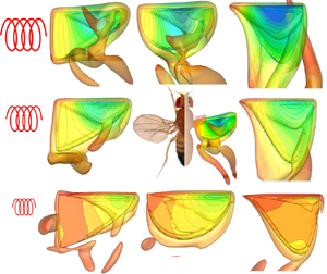
Eight different wing shapes are considered to systematically explore the interaction between wing-hinge properties and wing planform, as shown in figure 2. Each wing shape is generated using the beta function ( $\beta (p, q)$) by varying the radius of the first moment of area
  $\bar {r}_{1}$. The equations for the wing-shape generation are adopted from Ellington (Reference Ellington1984a)
 $$\begin{gather} \bar{r}_k^k=\int_{0}^{1} \bar{c} (\bar{r}^k) \,{\rm d} \bar{r}, \quad \bar{r}_2=0.929\left(\bar{r}_{1}\right)^{0.732}, \end{gather}$$
 $$\begin{gather}p=\bar{r}_{1}\left(\frac{\bar{r}_{1}\left(1-\bar{r}_{1}\right)}{\bar{r}_{2}^{2}-\bar{r}_{1}^{2}}-1\right),\quad q=\left(1-\bar{r}_{1}\right)\left(\frac{\bar{r}_{1}\left(1-\bar{r}_{1}\right)}{\bar{r}_{2}^{2}-\bar{r}_{1}^{2}}-1\right), \end{gather}$$
 $$\begin{gather}\beta(p, q)=\int_{0}^{1} \bar{r}^{p-1}(1-\bar{r})^{q-1} \,{\rm d} \bar{r}, \quad \bar{c}=\frac{\bar{r}^{p-1}(1-\bar{r})^{q-1}}{\beta(p, q)}, \end{gather}$$
where  $\bar {c}$ is the wing chord normalised by
  $c$ and
  $\bar {r}$ is the spanwise distance from the wing root normalised by
  $L$;
$L$;  $\bar {r}_k$ is the non-dimensional radius of the
  $k$th moment of the wing area. The values of
  $\bar {r}_1$ chosen for wing-shape generation are varied between
  $0.39$ and
  $0.63$, including the range of 0.43 and 0.6 for most insect wings (Ellington Reference Ellington1984a; Bhat et al. Reference Bhat, Zhao, Sheridan, Hourigan and Thompson2019a; Wang & Tian Reference Wang and Tian2020). The wing shapes are modelled with a constant planform area
  $A$, aspect ratio
  $AR$, wingspan
  $L$ and the mean chord length
  $c$ (
$c$ ( $c = L/AR$) for all cases to easily cross-compare performance metrics between them. As
  $\bar {r}_1$ increases, the planform area of the wing shifts further outboard from the wing root. The value
  $AR=2.96$ is chosen because previous studies on rigid wing shapes with prescribed flapping kinematics (Shahzad et al. Reference Shahzad, Tian, Young and Lai2016) have shown that maximum power economy is achieved at this aspect ratio independent of
  $Re$ and
  $\bar {r}_1$. The values of
  $J_{yy}$,
  $J_{zz}$ and
  $J_{yz}$ for different wings are provided in Appendix B.2.

Figure 2. Eight different wing planforms have been obtained by varying  $\bar {r}_{1}$: (a)
  $\bar {r}_1=0.39$; (b)
  $\bar {r}_1=0.43$;(c)
  $\bar {r}_1=0.48$; (d)
  $\bar {r}_1=0.53$; (e)
  $\bar {r}_1=0.565$; ( f)
  $\bar {r}_1=0.58$; (g)
  $\bar {r}_1=0.605$; (h)
  $\bar {r}_1=0.63$.
The far-field boundary condition is applied at the external boundaries of the computational domain and the no-slip boundary condition is applied on the wing surface. Zero velocity and constant pressure are specified as the initial condition of the flow. The initial stroke position of the wing is at  $-\phi _A/2$ with zero velocity, and the initial pitching angle is the rest pitching angle. Note that we have conducted simulations to verify that the results are independent of the initial condition of the wing (see Appendix B.3).
3. Numerical method
The flow over a flapping wing is solved by an immersed boundary-lattice Boltzmann method (IB–LBM) FSI solver based on the three-dimensional nineteen discrete velocity (D3Q19) lattice Boltzmann method (LBM) with a multi-relaxation-time (MRT) model for modelling the fluid dynamics and the feedback immersed-boundary method (IBM) for handling the boundary conditions at the fluid-solid interface. In the LBM, the macroscopic dynamics of the fluid is the result of the statistical behaviour of the fluid particles, which is described by the distribution function  $g_i(\boldsymbol {x},t)$ according to (Lallemand & Luo Reference Lallemand and Luo2000; Luo et al. Reference Luo, Liao, Chen, Peng and Zhang2011)
 \begin{equation} g_i\left(\boldsymbol{x}+\boldsymbol{e}_i{\rm \Delta} t, t+{\rm \Delta} t\right)-g_i \left(\boldsymbol{x},t\right)=\varOmega_i\left(\boldsymbol{x},t\right)+ {\rm \Delta} t G_i, \end{equation}
where  $g_i(\boldsymbol {x},t)$ is the distribution function for particles with velocity
  $\boldsymbol {e}_i$ at position
  $\boldsymbol {x}$ and time
  $t$,
$t$,  ${\rm \Delta} t$ is the time increment,
  $\varOmega _i(\boldsymbol {x},t)$ is the collision operator and
  $G_i$ is the forcing term accounting for the body force
  $\boldsymbol {f}$. The D3Q19 model (D'Humieres et al. Reference D'Humieres, Ginzburg, Krafczyk, Lallemand and Luo2002) is used on a cube lattice. Compared with the single-relaxation-time collision model, the MRT model has been proven to be numerically more stable (Lallemand & Luo Reference Lallemand and Luo2000; Xu et al. Reference Xu, Tian, Young and Lai2018). Therefore, the MRT collision model is adopted here and is given by (Lallemand & Luo Reference Lallemand and Luo2000)
 \begin{equation} \varOmega_i={-}(\boldsymbol{M}^{{-}1}\boldsymbol{S}\boldsymbol{M})_{ij} [g_i(\boldsymbol{x},t)-g_i^{eq}(\boldsymbol{x},t)],\end{equation}
where  $\boldsymbol {M}$ is a
  $19\times 19$ transform matrix, and
  $\boldsymbol {S}=diag(\tau _0,\tau _1,\ldots,\tau _{18})^{-1}$ is a non-negative diagonal relaxation matrix. The determination of
  $\boldsymbol {S}$ in a three-dimensional model can be found in D'Humieres et al. (Reference D'Humieres, Ginzburg, Krafczyk, Lallemand and Luo2002). The equilibrium distribution function
  $g_i^{eq}$ is defined as
 \begin{equation} g^{eq}_i=\rho\omega_i\left[1+\frac{\boldsymbol{e_i} \boldsymbol{\cdot}\boldsymbol{u}}{c^2_s}+ \frac{\boldsymbol{uu}:(\boldsymbol{e}_i\boldsymbol{e}_i-c^2_s\boldsymbol{I})}{2c^4_s}\right], \end{equation}
where  $c_s={\rm \Delta} x/(\sqrt {3}{\rm \Delta} t)$ is the speed of sound,
  ${\rm \Delta} x$ is the lattice spacing,
  $\boldsymbol {I}$ is the unit tensor and the weighting factors
  $\omega _i$ are given by
  $\omega _0=1/3$,
  $\omega _{1-6}=1/18$ and
  $\omega _{7-18}=1/36$. The velocity
  $\boldsymbol {u}$, mass density
  $\rho$ and pressure
  $p$ can be obtained according to
 \begin{equation} \rho=\sum_{i}g_i,\quad p=\rho c_s^2, \quad \mathrm{and} \quad \boldsymbol{u}=\left(\sum_{i}\textbf{e}_i g_i+\frac{1}{2}\, \boldsymbol{f}{\rm \Delta} t\right)\Bigg/\rho, \end{equation}
respectively. The force scheme proposed in Guo, Zheng & Shi (Reference Guo, Zheng and Shi2002) is adopted to determine  $G_i$
$G_i$
 $$\begin{gather} G_i=[\boldsymbol{M}^{{-}1}(\boldsymbol{I}-\boldsymbol{S}/2)\boldsymbol{M}]_{ij}F_i, \end{gather}$$
 $$\begin{gather}F_i=\left(1-\frac{1}{2\tau}\right)\omega_i\left[\frac{\boldsymbol{e}_i-\boldsymbol{u}}{c^2_s}+ \frac{\boldsymbol{e}\boldsymbol{\cdot}\boldsymbol{u}}{c^4_s} \boldsymbol{e}_i\right]\boldsymbol{\cdot}\boldsymbol{f}, \end{gather}$$
where  $\tau$ is the non-dimensional relaxation time.
The feedback IBM (e.g. Goldstein, Handler & Sirovich Reference Goldstein, Handler and Sirovich1993; Huang & Tian Reference Huang and Tian2019; Huang et al. Reference Huang, Tian, Young and Lai2021b, Reference Huang, Liu, Wang, Ravi, Young, Lai and Tian2022) is adopted to handle the no-slip boundary conditions on the flapping wing. In this method, the body force  $\boldsymbol {f}$ is added in the Navier–Stokes equations to mimic a boundary condition according to
 $$\begin{gather} \boldsymbol{f}(\boldsymbol{x},t)={-}\int \boldsymbol{F}_{ib}(s,t) \delta (\boldsymbol{x}-\boldsymbol{X}(s,t))\,{\rm d} A, \end{gather}$$
 $$\begin{gather}\boldsymbol{F}_{ib}(s,t)=\kappa \rho(\boldsymbol{x},t) (\boldsymbol{U}_{ib}(s,t)-\boldsymbol{U}(s,t)), \end{gather}$$
 $$\begin{gather}\boldsymbol{U}_{ib}(s,t)=\int \boldsymbol{u}(x,t)\delta (\boldsymbol{x}-\boldsymbol{X}(s,t))\,{\rm d}\kern0.7pt\boldsymbol{x}, \end{gather}$$
where  $\boldsymbol {F}_{ib}(s,t)$ is the Lagrangian force density,
  $dA$ is the element surface area of the immersed boundary,
  $\delta (\boldsymbol {x}-\boldsymbol {X}(s,t))$ is Dirac's delta function,
  $\boldsymbol {x}=(x^{\prime },y^{\prime },z^{\prime })$ is the coordinate of the fluid lattice nodes,
  $\boldsymbol {X}$ is the coordinate of the structure (i.e. the flapping wing here),
  $\kappa$ is the feedback coefficient and is set to
  $\kappa =2$ m s
 $^{-1}$ in the LBM simulations (Huang et al. Reference Huang, Tian, Young and Lai2021b, Reference Huang, Liu, Wang, Ravi, Young, Lai and Tian2022),
  $\boldsymbol {U}_{ib}(s,t)$ is the immersed-boundary velocity obtained by an interpolation at the immersed boundary and
  $\boldsymbol {U}(s,t)$ is the velocity of the wing. The 4-point discrete delta function
  $\delta _h(\boldsymbol {x}-\boldsymbol {X}(s,t))$ is used to approximate the Dirac delta function (Peskin Reference Peskin2002)
 $$\begin{gather} \delta_h(\boldsymbol{x}-\boldsymbol{X}(s,t))= \frac{1}{{\rm \Delta} x^{\prime} {\rm \Delta} y^{\prime} {\rm \Delta} z^{\prime}}\zeta \left(\frac{x^{\prime}-X(s,t)}{{\rm \Delta} x^{\prime}}\right) \zeta\left(\frac{y^{\prime}-Y(s,t)}{{\rm \Delta} y^{\prime}}\right) \zeta\left(\frac{z^{\prime}-Z(s,t)}{{\rm \Delta} z^{\prime}}\right), \end{gather}$$
 $$\begin{gather}\zeta({r})=\left\{\begin{array}{ll} \dfrac{1}{8}\left(3-2|r|+\sqrt{1+4|r|-4r^2}\right), & 0\leq |r|\leq 1, \\ \dfrac{1}{8}\left(5-2|r|-\sqrt{-7+12|r|-4r^2}\right), & 1\leq |r|\leq 2, \\ 0, & |r|>2. \end{array}\right. \end{gather}$$
The numerical method used here has been extensively validated (e.g. Xu et al. Reference Xu, Tian, Young and Lai2018; Ma et al. Reference Ma, Wang, Young, Lai, Sui and Tian2020; Huang Reference Huang2021; Huang et al. Reference Huang, Mazharmanesh, Tian, Young, Lai and Ravi2021a,Reference Huang, Tian, Young and Laib, Reference Huang, Liu, Wang, Ravi, Young, Lai and Tian2022; Liu, Tian & Feng Reference Liu, Tian and Feng2022b) for external and internal flows. The velocity error, the spurious flow penetration and their consequences in external and internal flows of the numerical method have been discussed in Huang et al. (Reference Huang, Liu, Wang, Ravi, Young, Lai and Tian2022). Here, the simulations of a rectangular flapping wing and a fruit fly flapping wing are used to further validate the computations for three-dimensional flapping-wing cases with grid and time-step-independence tests (see Appendix B). To reduce the computational effort, a multi-block LBM (Yu, Mei & Shyy Reference Yu, Mei and Shyy2002; Xu et al. Reference Xu, Tian, Young and Lai2018; Liu et al. Reference Liu, Tian and Feng2022b) has been implemented to provide a high-resolution Cartesian grid near the solid body, with relatively lower resolutions in the far field. The computational domain has a size of  $30c \times 30c \times 30c$. Four blocks of grid are used, with a minimum grid size of
  $0.04c$ around the wing and the maximum grid size of
  $0.32c$ in the far field, resulting in a total grid number of
  $7.25\times 10^6$. The determination of the finest fluid grid size is based on the two validation cases shown in Appendix B. The grid size of the wing is half of the finest fluid grid size (i.e.
  $0.02c$) which is required by the IBM employed here. The far-field boundary conditions along six sides of the computational domain are set to be the Dirichlet boundary conditions for the velocity and pressure, which produce almost identical results as the Neumann boundary conditions due to the large computational domain used. The in-house solver is parallelised by a hybrid open multi-processing (OpenMP) and open message-passing interface (OpenMPI). Six stroke cycles are simulated to ensure that all force histories (e.g.
  $C_D$ and
  $C_L$) and kinematics are periodic, and the time-averaged values are calculated over the last cycle. Validation has been conducted to show that the cycle-to-cycle variations in
  $C_L$ and
  $C_D$ are negligible, as shown in Appendix B.4.
4. Results and discussion
4.1. Flight performance on the plane of  $\bar {r}_1$ and $Ch$


The flight performance of the wing measured by cycle-averaged lift coefficient  $\bar {C}_L$ and power economy
  $PE$ on the plane of
  $\bar {r}_1$ and
  $Ch$ is shown in figure 3, where several interesting results are obtained. Firstly,
  $\bar {C}_L$ increases with
  $\bar {r}_1$ when
  $Ch<0.15$ where the passive pitching is small. This behaviour is similar to the discussion for rigid wings (Ellington Reference Ellington1984b; Shahzad et al. Reference Shahzad, Tian, Young and Lai2016; Bhat et al. Reference Bhat, Zhao, Sheridan, Hourigan and Thompson2019b), which is understandable as the area of the wing is shifted towards the wingtip when
  $\bar {r}_1$ increases (see also figure 2) generating increasing aerodynamic forces. Secondly, when
  $Ch$ is large (e.g.
  ${\ge }0.2$),
  $\bar {C}_L$ first increases and then decreases with
  $\bar {r}_1$. The decrease of
  $\bar {C}_L$ is caused by the large passive pitching and the inertia force during stroke reversal, which have a significant negative effect on lift generation. This observation is consistent with the results obtained with wings modelled by flexible plates of low mass ratio (
 $M_c\le 1$) and aspect ratio (
 $AR<3.0$) (Shahzad et al. Reference Shahzad, Tian, Young and Lai2018a,Reference Shahzad, Tian, Young and Laib), and the compliant membrane wings (Gehrke et al. Reference Gehrke, Richeux, Uksul and Mulleners2022; Mathai et al. Reference Mathai, Tzezana, Das and Breuer2022). Such complex behaviour is because flexibility becomes important at large
  $Ch$, and the FSI system undergoes complex power synchronisation, which will be further discussed in § 4.2. Thirdly, when
  $Ch$ increases from
  $0.05$ to
  $0.6$,
  $\bar {C}_L$ first increases and then decreases, with the peak located in the band of
  $0.05\le Ch \le 0.2$. This observation is consistent with the studies with wings modelled by flexible plates (see e.g. Dai et al. Reference Dai, Luo and Doyle2012; Tian et al. Reference Tian, Luo, Song and Lu2013; Shahzad et al. Reference Shahzad, Tian, Young and Lai2018b). Overall, a high
  $\bar {r}_1$ (
 ${\geq }0.565$) and a low
  $Ch$ (
 ${\approx }0.1$) is useful in maximising
  $\bar {C}_L$ with an optimal value of
  ${\approx }0.67$. Finally, the behaviours of
  $PE$ in relation to
  $Ch$ are similar to
  $\bar {C}_L$, but its maximum value (
 ${\approx }0.71$) is obtained with
  $\bar {r}_1\approx 0.45$ and
  $Ch\approx 0.2$. This
  $\bar {r}_1$ value is very close to that of hawkmoth wings, which has been reported to be
  $\bar {r}_1\approx 0.47$ (Willmott & Ellington Reference Willmott and Ellington1997). However, in relation to
  $\bar {r}_1$,
  $PE$ shows negligible changes for
  $Ch<0.15$. This will be further investigated in § 4.3.

Figure 3. Flight performance on the plane of  $\bar {r}_1$ and
  $Ch$: (a) mean lift coefficient
  $\bar {C}_L$, and (b) power economy
  $PE$.
$PE$.
We should point out that, even though the above observations are obtained at  $Re=300$,
  $M_c=1.0$ and a specific wing shape, they can be generalised to other conditions (e.g. different
  $Re$ and
  $M_c$), with the optimal values and locations dependent on these conditions. This statement is made based on the results from previous studies. Specifically, the optimal
  $\bar {C}_L$ is larger, but the optimal
  $PE$ is smaller for higher
  $AR$, as reported by Shahzad et al. (Reference Shahzad, Tian, Young and Lai2018a), who considered flexible wings at
  $Re=400$. Moreover, the optimal locations of
  $\bar {C}_L$ and
  $PE$ are shifted to larger
  $\bar {r}_1$ for higher
  $AR$ (Shahzad et al. Reference Shahzad, Tian, Young and Lai2018a). In addition, insects may fly close to, but not exactly in, the optimal region. For example, the wings of fruit flies are found to be of
  $\bar {r}_1 \approx 0.53$ (Meng, Liu & Sun Reference Meng, Liu and Sun2017) and
  $Ch \approx 0.27$ (Lei & Li Reference Lei and Li2020). According to figure 3,
  $\bar {C}_L=0.43$ might be just sufficient to balance their weight and
  $PE \approx 0.58$ might be the near-optimal power economy. Overall, the current analysis highlights the strong influence of the coupled effects of wing shape and pitching spring stiffness on wing performance, which will be helpful for designing the flapping-wing flyers and further explain the mechanisms of insect flight.
To summarise this section, two distinct regions of maximum lift production and efficiency are identified. It is found that a high  $\bar {r}_1$ (
 ${\geq }0.565$) and a low
  $Ch$ (
 ${\approx }0.1$) is useful in maximising
  $\bar {C}_L$, and the power economy is maximised for wings with lower
  $\bar {r}_1$ (
 ${\approx }0.45$) near
  $Ch=0.2$.
4.2. Effects of the torsional spring stiffness
To discuss the mechanisms of high lift generation and flight performance, we present the results obtained by varying  $Ch$ for three values of
  $\bar {r}_1$ (0.39, 0.48 and 0.58). The forces, power economy, passive pitching and power components are particularly analysed.
We first discuss  $\bar {C}_L$,
  $\bar {C}_D$ and
  $PE$, as shown in figure 4. The trends of
  $\bar {C}_L$ and
  $PE$ are similar when
  $Ch$ increases from 0.05 to 0.6, as introduced in § 4.1. The peak values of
  $\bar {C}_L$ are approximately 0.36, 0.52 and 0.65 for
  $\bar {r}_1=0.39$, 0.48 and 0.58, respectively (see figure 4a). For all three
  $\bar {r}_1$ values, the highest value of
  $\bar {C}_L$ is observed between
  $Ch=0.1$ and
  $0.15$, suggesting an optimum range of
  $Ch$ to achieve the highest possible
  $\bar {C}_L$. The exact value of the optimum
  $Ch$ is found to vary within this small range with a change in the wing shape. For all the wings,
  $\bar {C}_D$ is observed to decrease monotonically with
  $Ch$, see figure 4(b). This observation is consistent with that of the two-dimensional hovering wing studied, for example, by Yin & Luo (Reference Yin and Luo2010). The decrease in
  $\bar {C}_D$ for a higher
  $Ch$ is caused by the larger passive pitching motion resulting in a smaller angle of attack. On the other hand,
  $PE$ increases with
  $Ch$, reaching its maximum value at
  $Ch\approx 0.15$ before decreasing with
  $Ch$, similar to the trend observed in
  $\bar {C}_L$ (see figure 4c). From
  $Ch=0.05$ to
  $0.15$,
  $PE$ is increased due to the increase of lift and the decrease of aerodynamic power (
 $\bar {C}_P$) caused by the softening of the spring. For
  $Ch>0.15$,
  $PE$ is found to decrease as the rate of the decrease in
  $\bar {C}_L$ is higher than that in
  $\bar {C}_P$. The significant and quick decrease of
  $\bar {C}_L$ is due to the negative lift caused by the delayed pitch for soft springs and the reduced size of the leading-edge vortex, which will be demonstrated in the analysis of wing kinematics and vortex structures.

Figure 4. Variations in (a)  $\bar {C}_L$, (b)
  $\bar {C}_D$ and (c)
  $PE$ are shown as functions of
  $Ch$ for three different wing shapes of
  $\bar {r}_1=0.39$, 0.48 and 0.58.
We then present the flapping and pitching power expenditures from various sources, as shown in figure 5, from which several important observations are obtained. Firstly, the flapping aerodynamic power dominates power consumption with peak values roughly 3 times those of the flapping inertial power. This is consistent with the definition of the mass ratio,  $M=M_c/AR\approx 1/3$, which indicates that the scale of the inertial forces is approximately 1/3rd of that of the aerodynamic forces. The exception is the case of
  $Ch=0.6$, where the spring is very soft, resulting in a much smaller aerodynamic force (thus much smaller aerodynamic power) and larger pitching inertial power compared with that of lower
  $Ch$ cases. Secondly, the flapping aerodynamic power almost always remains positive due to a low mass ratio considered and the continuous work required to overcome the drag. The exception is the case of a very stiff wing (i.e.
  $Ch=0.05$) with a negative aerodynamic power just before the end of each half-stroke, similar to that observed with a two-dimensional flapping wing in Tian et al. (Reference Tian, Luo, Song and Lu2013), and is caused by the deceleration of the stroke motion. According to two-dimensional simulations (Yin & Luo Reference Yin and Luo2010; Tian et al. Reference Tian, Luo, Song and Lu2013), the cases with high mass ratios could also generate negative aerodynamic power due to a delayed rotation. Normally, the flapping aerodynamic power reaches its maximum value at around midstroke (e.g.
  $tf=5.25$ and
  $tf=5.75$), where the drag and the stroke velocity are maximal. Thirdly, for pitching motion, the elastic power of the spring balances the pitching–inertial and pitching–aerodynamic powers and, thus, no net power consumption is observed. Fourthly, the flapping aerodynamic power decreases monotonically with
  $Ch$ similar to the trend observed in
  $C_D$ (figure 4b), while the flapping and pitching inertial powers increase monotonically with
  $Ch$ because the wing of higher
  $Ch$ travels over a larger
  $\theta$ range, resulting in higher
  $\dot \theta$ and
  $\ddot \theta$. As a result, the pitching elastic power increases correspondingly to balance the increased pitching inertial and aerodynamic powers.

Figure 5. Time traces of power coefficients ( $CP$ values) at
  $\bar {r}_1=0.48$ for six different spring stiffness values indicated by
  $Ch=0.05$,
  $Ch=0.1$,
  $Ch=0.15$,
  $Ch=0.2$,
  $Ch=0.3$ and
  $Ch=0.6$.
  $CP_{iner}^{flap}$: flapping inertial power coefficient;
  $CP_{aero}^{flap}$: flapping aerodynamic power coefficient;
  $CP_{iner}^{pitch}$: pitching inertial power coefficient;
  $CP_{aero}^{pitch}$: pitching aerodynamic power coefficient;
  $CP_{spri}^{pitch}$: pitching elastic power coefficient;
  $CP_{total}$: total power coefficient.
  $CP=power/(0.5 \rho U^3 A)$, where
  $A$ is the surface area of the wing. Here,
  $tf$ is non-dimensional time, normalised by flapping frequency
  $f$.
$f$.
Finally, for  $Ch\in [0.1$,
  $0.2]$, a nearly in-phase synchronisation (with a phase difference
  ${\rm \Delta} \phi _{flap} \in [18^\circ, 30^\circ ]$ as measured in figure 6a) is observed between the flapping aerodynamic power and the total system input power. Simultaneously, an anti-phase synchronisation (with a mean phase difference
  ${\rm \Delta} \phi _{pitch} \approx 180^\circ$ as measured in figure 6a) between the pitching elastic power and the pitching aerodynamic and inertial powers is observed. The nearly in-phase synchronisation between the flapping aerodynamic power and the total system input power ensures that the total system input power is mainly used to drive the flapping motion without being wasted in other power components, while the anti-phase synchronisation between the pitching powers ensures that the pitching aerodynamic and inertial powers are fully stored in the elastic pitching power and vice versa. The phase difference between flapping aerodynamic power and the total system input power shows an increasing trend as the increase of
  $Ch$. The nearly in-phase synchronisation between the flapping aerodynamic power and the total system input power is also reflected by the timing of pitch rotation, which will be further analysed below. As shown in figure 6(b), the maximal absolute value of the peak pitching elastic power occurs at
  $Ch\in [0.1$,
  $0.2]$, indicating an efficient storage and release process of the elastic energy in this region. This is consistent with the work by Cai et al. (Reference Cai, Xue, Kolomenskiy, Xu and Liu2022) who reported that the elastic storage minimises the high energetic cost of flapping wings. For
  $Ch=0.05$, the wing is stiff, and while the synchronisation between flapping and pitching is similar to that required for high lift, the wing's minimal angle of attack is much higher than
  $45^{\circ }$ where the optimum lift is produced. In addition, the drag is high for
  $Ch=0.05$ resulting in a low power economy. Wings with
  $Ch \in [0.1, 0.2]$ produce an optimal lift and a relatively small drag as the wing experiences the minimal angle of attack
  ${\approx }45^{\circ }$, which will be analysed and discussed in the following parts of this section.

Figure 6. (a) Phase difference ( ${\rm \Delta} \phi$) of power coefficients, as a function of
  $Ch$. Here,
  ${\rm \Delta} \phi _{flap}$: phase difference between the flapping aerodynamic power and the total system input power;
  ${\rm \Delta} \phi _{pitch}$: mean phase difference between the pitching elastic power and the pitching aerodynamic and inertial powers. (b) The absolute value of the peak pitching elastic power.
To further study the reasons for high  $\bar {C}_L$ and
  $PE$ with various
  $Ch$, the time histories of
  $C_L$,
  $C_D$, the pitching angle
  $\theta$ and the corresponding angle of attack
  $\alpha$ are shown in figure 7; the minimal angle of attack
  $\alpha _{min}$ and the pitch rotation delay
  $\delta _{\alpha }$ are shown in figure 8. It should be noted that the pitching angle
  $\theta$ about the pitching axis is measured with reference to the
  $z$-axis. Hence, the angle of attack
  $\alpha$ is defined as
 \begin{equation} \alpha=\begin{cases} 90^{{\circ}}-\theta, & \text{if $\dot{\phi}<0$},\\ 90^{{\circ}}+\theta, & \text{if $\dot{\phi}\geq 0$}. \end{cases} \end{equation}
Various quasi-steady models correlate  $C_L$ and
  $\alpha$ as
  $C_L=f[\sin (2\alpha )]$ (Dickinson et al. Reference Dickinson, Lehmann and Sane1999; Sane & Dickinson Reference Sane and Dickinson2001, Reference Sane and Dickinson2002; Wang, Goosen & van Keulen Reference Wang, Goosen and van Keulen2016). Thus,
  $C_L$ is expected to be maximum when
  $\alpha \approx 45^\circ$, which is slightly higher than that for a translated flat-plate wing (Taira & Colonius Reference Taira and Colonius2009). On the other hand,
  $C_D$ is expected to increase with
  $\alpha$. As the softer springs at higher
  $Ch$ result in lower
  $\alpha$ values, the corresponding
  $C_D$ is also lower, irrespective of
  $\bar {r}_1$. For a higher
  $\bar {r}_1$, a larger area is available outboard to support a larger leading-edge vortex (LEV), which results in higher suction magnitudes beneath the LEV. Thus, values of both
  $C_L$ and
  $C_D$ are slightly more enhanced in magnitude compared with those at lower
  $\bar {r}_1$.

Figure 7. Time traces of  $\theta$,
  $\alpha$,
  ${C}_{L}$ and
  $C_D$ are shown for passively pitching wings with four different
  $Ch$ values. The left column shows the results for the wing of
  $\bar {r}_1=0.39$ and the right column shows the results for the wing of
  $\bar {r}_1=0.58$. Data for fruit fly kinematics are obtained from Fry, Sayaman & Dickinson (Reference Fry, Sayaman and Dickinson2005). Here,
  $tf$ is the non-dimensional time. Note that the results are shown for the 6th flapping cycle at which point the forces and kinematics are periodic. Markers are shown at every 10th time step in the calculations. (a) Time traces of
  $\theta$ for
  $\bar {r}_1=0.39$. (b) Time traces of
  $\theta$ for
  $\bar {r}_1=0.58$. (c) Time traces of
  $\alpha$ for
  $\bar {r}_1=0.39$. (d) Time traces of
  $\alpha$ for
  $\bar {r}_1=0.58$. (e) Time traces of
  $C_L$ for
  $\bar {r}_1=0.39$. ( f) Time traces of
  $C_L$ for
  $\bar {r}_1=0.58$. (g) Time traces of
  $C_D$ for
  $\bar {r}_1=0.39$. (h) Time traces of
  $C_D$ for
  $\bar {r}_1=0.58$.

Figure 8. Contours of  $\alpha _{min}$ reached in a flapping stroke are shown in (a) on the map of
  $\bar {r}_1$ and
  $Ch$, where the white colour represents
  $\alpha _{ref}\approx 45^{\circ }$. The contours of pitch-rotation delay (
 $\delta _{\alpha }$) as a percentage of the flapping period are shown in (b) on the map of
  $\bar {r}_1$ and
  $Ch$.
$Ch$.
The instantaneous values of  $C_L$ are also affected by the synchronisation in the flapping and pitching kinematics. The delay in pitch reversal
  $\delta _{\alpha }$ is calculated as the phase difference between the flapping stroke reversal and the time when
  $\alpha$ reaches the neutral position of
  $90^{\circ }$. From figures 7 and 8, a few interesting results are obtained. Pitch reversal is more delayed with increasing
  $Ch$, as seen in figures 7(a) and 7(b). The delayed pitch causes the instantaneous
  $\alpha$ after the flapping stroke reversal to be greater than
  $90^{\circ }$, which results in negative
  $C_L$ due to the wing being pushed down by the fluid on the wing pressure side. Additionally, the rapid pitch-down motion observed prior to
  $t/T=5.2$ results in high circulation around the wing that contributes to a significantly high downward force. Thus,
  $Ch=0.6$ shows negative values of
  $C_L$ during a part of a stroke, which is responsible for a lower
  $\bar {C}_L$ of a complete cycle, see figures 7(e) and 7( f). Close to
  $t/T=5.2$, the pitch-down motion decelerates, followed by the pitch-up motion, which contributes to a positive lift even at low values of
  $\alpha$ close to
  $t/T=5.35$. Irrespective of the wing shape, the pitching amplitude of the wing during the midstroke is observed to increase with
  $Ch$; consequently, the angle of attack
  $\alpha$ reached near the midstroke is lower, see figures 7(c) and 7(d). The case
  $Ch=0.15$ experiences the highest instantaneous
  $C_L$, as the wing nearly maintains
  $\alpha \approx 45^{\circ }$ (which is also very close to
  $\alpha _{min}$, see figures 7(c) and 7(e)), which has been shown in previous studies to be the most effective
  $\alpha$ for lift generation (e.g. Dickinson Reference Dickinson1994; Dickinson et al. Reference Dickinson, Lehmann and Sane1999). The wing of
  $\bar {r}_1=0.58$ approaches significantly lower values of
  $\alpha _{min}$. Combined with a delayed pitch, this behaviour results in large negative instantaneous values of
  $C_L$ as well as an overall lower
  $\bar {C}_L$. Typically, fruit fly wings have
  $\bar {r}_1\approx 0.53$ (Meng et al. Reference Meng, Liu and Sun2017) and
  $Ch\approx 0.27$ (Lei & Li Reference Lei and Li2020). The time traces of
  $\theta$ and
  $\alpha$ for a hovering fruit fly from Fry et al. (Reference Fry, Sayaman and Dickinson2005) are compared in figures 7(b) and 7(d) along with a wing with
  $\bar {r}_1=0.58$. The variations in
  $\theta$ and
  $\alpha$ for a fruit fly wing appear to follow the time traces between the cases
  $Ch=0.15$ and 0.3, which are not in, but close to, the optimal lift region. For all wing shapes,
  $C_D$ decreases monotonically with
  $Ch$, caused by the reduced angle of attack for softer springs, see figures 7(g) and 7(h).
The minimal angle of attack  $\alpha _{min}$ is found to decrease continuously with increasing
  $Ch$, see figure 8(a). This is expected since a softer spring will allow the wing to deform more in pitch from its neutral position. Wings with
  $Ch$ in the range of
  $[0.1, 0.2]$ produce a maximum
  $C_L$ (figure 4a) and experience
  $\alpha _{min}\approx 45^{\circ }$. The value of
  $Ch$ required to achieve
  $\alpha _{min}=45^{\circ }$ reduces with
  $\bar {r}_1$. This is because, for a higher
  $\bar {r}_1$, the larger area available outboard to support the LEV results in increased suction pressure, whose resultant force makes the wing tilt more than that for a lower
  $\bar {r}_1$. Consequently, the region of
  $\alpha _{min}=45^{\circ }$ in figure 8(a) is observed to decrease linearly on the map of
  $\bar {r}_1$ and
  $Ch$. This also explains why the region of high
  $\bar {C}_L$ in figure 3(a) is shifted to lower
  $Ch$ at high
  $\bar {r}_1$ values.
The delay in pitch reversal  $\delta _{\alpha }$ is seen to increase with
  $Ch$ for all the examined wing shapes, see figure 8(b). For stiffer springs with
  $Ch<0.15$, the pitch rotation is advanced with respect to the flapping stroke (i.e.
  $\delta _{\alpha }<0$), whereas for softer springs, the pitch rotation is delayed (i.e.
  $\delta _{\alpha }>0$). As has been previously reported by Dickinson et al. (Reference Dickinson, Lehmann and Sane1999) and Sane & Dickinson (Reference Sane and Dickinson2001), the advanced pitch can be useful in achieving higher lift and the delayed pitch may be detrimental. On the other hand, the advanced pitch also results in a higher
  $C_D$. This confirms the in-phase synchronisation between the flapping aerodynamic power and the total system input power. Similarly, the anti-phase synchronisation between the elastic pitching power and the pitching aerodynamic and inertial powers is reflected in
  $\delta _{\alpha }\approx 0^{\circ }$ for optimal
  $PE$ cases (see the
  $Ch=0.15$ case in figure 5). The region of
  $\delta _{\alpha }=0$ represents the exact synchronisation between the flapping and pitching motions. This is the region where the highest power economy can be observed for a given wing shape or stiffness, which explains the variations in
  $PE$ shown in figure 3(b). Note that the cases with high flexibility, i.e.
  $Ch>0.45$ and
  $\bar {r}_1>0.6$ have the wing rotated up to and beyond
  $\alpha _{min}=0^{\circ }$, causing the lift and drag to be highly unstable during a stroke. Overall,
  $Ch \in [0.1,0.2]$ may be ideal for simultaneously obtaining
  $\alpha _{min}=45^{\circ }$ to maximise
  $\bar {C}_L$ and
  $\delta _{\alpha }\leq 0$ to maximise
  $PE$.
$PE$.
To summarise this section, the lift production is optimal at  $0.05 < Ch \leq 0.2$ and larger
  $\bar {r}_1$, where the minimum angle of attack is around
  $45^\circ$ at the midstroke, while the best configuration for the maximum
  $PE$ is achieved at
  $\bar {r}_1=0.45$ and
  $Ch=0.2$, where the flapping aerodynamic power is approximately three times in magnitude of the flapping inertial power.
The optimal performance measured by the power economy is obtained for those cases where two important power synchronisations occur: anti-synchronisation of the pitching elastic power and the pitching aerodynamic and inertial powers and nearly in-phase synchronisation of the flapping aerodynamic power and the total input power of the system.
4.3. Wing-shape effects
The effects of wing shape on the aerodynamic performance are explored by varying  $\bar {r}_1$. The variation in the cycle-averaged lift coefficient (
 $\bar {C}_L$) as a function of
  $\bar {r}_1$ using three different torsional springs corresponding to
  $Ch = 0.05$,
  $0.15$ and
  $0.45$, is shown in figure 9(a). For the case of the stiffest spring at the wing hinge (i.e.
  $Ch=0.05$),
  $\bar {C}_L$ increases monotonically with
  $\bar {r}_1$. This is in concurrence with previous observations on actively pitching rigid wing shapes with prescribed kinematics. It has been shown that the larger outboard area of a high-
 $\bar {r}_1$ wing supports the larger LEV that is responsible for creating higher suction on the wing surface, resulting in higher lift (Shahzad et al. Reference Shahzad, Tian, Young and Lai2018a; Bhat et al. Reference Bhat, Zhao, Sheridan, Hourigan and Thompson2019b). However, this observation does not hold true for passively pitching wings with softer torsional springs, see figure 9(a). For wings with softer springs (i.e.
  $Ch=0.15$ and
  $Ch=0.45$),
  $\bar {C}_L$ increases with
  $\bar {r}_1$ only until a certain
  $\bar {r}_1$, beyond which it starts decreasing. The value of
  $\bar {r}_1$ giving a maximum
  $\bar {C}_L$ changes with
  $Ch$:
$Ch$:  $\bar {C}_{Lmax}=0.573$ at
  $\bar {r}_1=0.565$ for
  $Ch=0.15$ and
  $\bar {C}_{Lmax}=0.187$ at
  $\bar {r}_1=0.48$ for
  $Ch=0.45$.

Figure 9. Variations in (a)  $\bar {C}_{L}$, (b)
  $\bar {C}_{D}$ and (c)
  $PE=\bar {C}_{L}/\bar {C}_{P}$ with
  $\bar {r}_1$ (wing shape) are shown for passively pitching wings with three different
  $Ch$ values.
Similar trends are also observed in the cycle-averaged drag coefficient ( $\bar {C}_D$), as shown in figure 9(b). For the stiffest hinge (i.e.
  $Ch=0.05$),
  $\bar {C}_D$ appears to increase monotonically with
  $\bar {r}_1$ but for less stiff hinges such as
  $Ch=0.15$ and
  $0.45$,
  $\bar {C}_D$ increases with
  $\bar {r}_1$ to a maximum after which it decreases with
  $\bar {r}_1$. Previous studies (e.g. Shahzad et al. Reference Shahzad, Tian, Young and Lai2018a) have shown that, for actively pitching rigid wings,
  $PE$ decreases with an increase in
  $\bar {r}_1$ due to an increased
  $\bar {C}_D$. However, for passively pitching wings, the observations are different, as can be seen in figure 9(c). For
  $Ch=0.05$, the increase in the outboard area with
  $\bar {r}_1$, together with a reducing angle of attack
  $\alpha$ approaching
  $45^{\circ }$, results in a greater increase in
  $\bar {C}_L$ than in
  $\bar {C}_D$, causing
  $PE$ to increase with
  $\bar {r}_1$ for
  $\bar {r}_1>0.43$. However, for
  $Ch=0.45$, both
  $\bar {C}_L$ and
  $\bar {C}_D$ are lower, resulting in the highest
  $PE$ (
 $0.466$) at
  $\bar {r}_1= 0.43$. For the medium-soft spring case (
 $Ch=0.15$) the balance between spring stiffness and aerodynamic contribution results in the highest
  $PE=0.662$, which remains virtually constant for
  $0.43\leq \bar {r}_1 \leq 0.565$.
Overall, the variation in  $PE$ appears to directly depend on the pitch-rotation delay caused by the power synchronisations, as discussed earlier. For
  $Ch=0.05$, the pitch rotation is advanced compared with the flapping motion, as can be seen in figure 8(b). At higher
  $\bar {r}_1$, the rotation is less advanced, which causes an increase in
  $PE$ seen here in figure 9(c). At
  $Ch=0.15$, the delay of
  $\delta _{\alpha }\approx 2.5\,\%$ is mostly unaffected by
  $\bar {r}_1$. Thus, the value of
  $PE$ also remains mostly unchanged. However, at a higher
  $Ch$, the pitch rotation is more delayed. It first decreases with
  $\bar {r}_1$, followed by an increase. Hence, the resulting
  $PE$ also shows a variation as shown for the case of
  $Ch=0.45$ in figure 9(c).
It can be seen that the choice of the wing shape to achieve the best possible hover performance, both in terms of  $\bar {C}_L$ and
  $PE$, is determined by the spring stiffness used for the passively pitching wings. The reasons behind the trends in
  $\bar {C}_L$ with various
  $\bar {r}_1$ are further analysed by comparing their time histories of the pitching angle
  $\theta$ and the corresponding angle of attack
  $\alpha$, as shown in figure 10.

Figure 10. Time traces of the pitching angle  $\theta$, angle of attack
  $\alpha$ and lift coefficient
  ${C}_{L}$ are shown for passively pitching wings with three different
  $\bar {r}_1$ values. The left column shows the results for
  $Ch=0.05$ and the right column shows the results for
  $Ch=0.45$. Here,
  $tf$ is non-dimensional time, normalised by flapping frequency
  $f$. Note that the results are shown for the 6th cycle at which point the forces and kinematics are periodic. Markers are shown at every 10th time step in the calculations. (a) Time traces of
  $\theta$ for
  $Ch=0.05$. (b) Time traces of
  $\theta$ for
  $Ch=0.45$. (c) Time traces of
  $\alpha$ for
  $Ch=0.05$. (d) Time traces of
  $\alpha$ for
  $Ch=0.45$. (e) Time traces of
  $C_L$ for
  $Ch=0.05$. ( f) Time traces of
  $C_L$ for
  $Ch=0.45$.
The pitching amplitude is observed to increase with  $\bar {r}_1$, as can be seen in figures 10(a) and 10(b). The corresponding variations in the angle of attack
  $\alpha$ are shown in figures 10(c) and 10(d). As
  $\alpha$ approaches
  $45^{\circ }$,
  $C_L$ is also observed to increase, in accordance with the quasi-steady models (Dickinson et al. Reference Dickinson, Lehmann and Sane1999; Sane & Dickinson Reference Sane and Dickinson2001, Reference Sane and Dickinson2002), as shown in figures 10(e) and 10( f). On the other hand, for a softer spring, i.e.
  $Ch=0.45$, the elastic energy from the spring is low and the pitching amplitudes are high, resulting in
  $\alpha <45^{\circ }$ during the midstroke (e.g.
  $tf=5.25$). Hence, the corresponding values of
  $C_L$ at midstroke are lower than those for
  $Ch=0.05$. Please note that for most cases,
  $\alpha$ reaches its minimum value before the midstroke and reduces thereafter even though the stroke velocity is still increasing. This is caused by the inertial force of the wing during stroke reversal (see e.g. Dai et al. Reference Dai, Luo and Doyle2012; Tian et al. Reference Tian, Luo, Song and Lu2013). Due to the large pitching motions experienced by the wing with a softer spring, there are also significant changes in the phase of pitch reversal, identified by the phase at which the wing crosses the
  $\alpha =90^{\circ }$ threshold. Instantaneous
  $C_L$ can assume significantly negative values near the midstroke for
  $\bar {r}_1=0.63$ and
  $Ch=0.45$ (see figure 10f) which contributes to the low
  $\bar {C}_L$ produced by the wing. The negative
  $C_L$ is due to the high negative pressure that develops near the trailing edge of the wing pressure side during stroke reversal (see supplementary movie 1 available at https://doi.org/10.1017/jfm.2023.821 for an animation of the time history of the lift coefficient and the corresponding vortex structures). The animation for
  $\bar {r}_1=0.63$ and
  $Ch=0.05$ is also provided for comparison (see supplementary movie 2).
The wing-shape effects can be better understood by observing the flow structures around the wing, as shown in figure 11. Here, the flow over wings of various  $\bar {r}_1$ for
  $Ch=0.05$ and
  $Ch=0.45$ is shown at the midstroke, i.e. at
  $tf=5.25$. The LEV, the dominant flow feature shown to be responsible for the high lift produced by flapping wings, is highlighted in all cases. Since the value of
  $\alpha$ at midstroke is higher with a stiffer spring (
 $Ch=0.05$) and is closer to 45
 $^{\circ }$, the size of the LEV over the wings is larger than the LEV that forms over the wing with a softer spring (
 $Ch=0.45$). The larger LEV creates a higher suction on the wing surface beneath the vortex. Moreover, the LEV is smaller near the root and increases in size in the spanwise direction. Hence, a larger outboard area of the wing with
  $\bar {r}_1=0.63$ supports a larger LEV, which results in a stronger suction. This explains the increase in
  $C_L$ with
  $\bar {r}_1$ for the wing with a stiff hinge (figure 9(a) for
  $Ch=0.05$) or fully prescribed kinematics (Combes & Daniel Reference Combes and Daniel2001; Shahzad et al. Reference Shahzad, Tian, Young and Lai2018a). For a softer spring with
  $Ch=0.45$, the suction pressure beneath the LEV increases with
  $\bar {r}_1$. However, beyond
  $\bar {r}_1=0.48$, the value of
  $\alpha$ at the midstroke also reduces significantly, causing the LEV to be smaller and weaker. In addition, the wing of
  $\bar {r}_1=0.63$ and
  $Ch=0.45$ rapidly pitches up (i.e. the trailing edge swings up) before
  $tf=5.2$, leading to a strong vortex at the bottom surface near the trailing edge (see figure 11f), and a strong deceleration occurs thereafter until
  $tf=5.25$ causing a strong inertia force downwards. Therefore, even with a larger outboard area and a positive angle of attack, the
  $\bar {r}_1=0.63$ wing produces smaller
  $\bar {C}_L$, as seen in figure 11( f). Overall, the variation in
  $C_L$ with
  $\bar {r}_1$ is found to be dependent largely on the torsional spring stiffness.

Figure 11. Vortices are visualised by semi-transparent iso-surfaces of the normalised Q-criterion ( $Q^{\ast }=100$) and the wing suction sides are coloured by the normalised pressure (
 $p^{\ast }=p/(\rho U^2)$) contours at the midstroke
  $tf=5.25$. (a–c) Represent the wings of
  $\bar {r}_1=0.39$, 0.48 and 0.63, respectively, with
  $Ch=0.05$.(d–f) Represent the same wings with
  $Ch=0.45$.
Power expenditures from various sources of four wing shapes  $\bar {r}_1=0.39$,
  $0.48$,
  $0.58$ and
  $0.63$ are further analysed in figure 12. For all four wing shapes, the flapping inertial power traces two nearly sinusoidal curves with the positive part being larger than the negative part, see figure 12. The positive flapping inertial power is used to accelerate the wing at the beginning of each stroke cycle (i.e. from
  $tf=5$ to
  $tf=5.25$), and the negative inertial power indicates the work done by the fluid on the wing to decelerate it after the midstroke (i.e. from
  $tf=5.25$ to
  $tf=5.5$). The pitching inertial power increases with
  $\bar {r}_1$, due to the significantly increased inertial contribution from flapping (i.e.
  $J_{zy}$). As a result, the pitching elastic power increases with
  $\bar {r}_1$ to balance the increased pitching inertial and pitching aerodynamic power.

Figure 12. Time traces of power coefficients ( $CP$ values) at
  $Ch=0.15$ for four different wing shapes of
  ${\bar {r}_1=0.39}$,
  ${\bar {r}_1=0.48}$,
  $\bar {r}_1=0.58$ and
  $\bar {r}_1=0.63$. Here,
  $CP_{iner}^{flap}$: flapping inertial power coefficient;
  $CP_{aero}^{flap}$: flapping aerodynamic power coefficient;
  $CP_{iner}^{pitch}$: pitching inertial power coefficient;
  $CP_{aero}^{pitch}$: pitching aerodynamic power coefficient;
  $CP_{spri}^{pitch}$: pitching elastic power coefficient;
  $CP_{total}$: total power coefficient. Power coefficient
  $CP=power/(0.5 \rho U^3 A)$, where
  $A$ is the surface area of the wing. Here,
  $tf$ is non-dimensional time, normalised by flapping frequency
  $f$.
$f$.
As  $\bar {r}_1$ increases from
  $0.39$ to
  $0.58$, the peak value of the flapping aerodynamic power increases by
  $42.50\,\%$ (i.e. from
  $1.20$ to
  $1.71$), followed by a minor decrease (
 $9.36\,\%$) as
  $\bar {r}_1$ increases to
  $0.63$. On the other hand, the flapping inertial power increases monotonically and significantly with
  $\bar {r}_1$ as the moment of inertia around the flapping axis (i.e.
  $J_{zz}$) is doubled (
 $J_{zz}=5.64$ and
  $11.38$ for
  $\bar {r}_1=0.39$ and
  $0.63$, respectively). At
  $Ch=0.15$, as shown in figure 9,
  $\bar {C}_D$ and
  $PE$ are roughly the same for different
  $\bar {r}_1$, with a
  $10.15\,\%$ increase of
  $\bar {C}_L$ for
  $\bar {r}_1=0.48$ and
  $\bar {r}_1=0.58$. The slight increase of
  $\bar {C}_L$ is at the cost of a significant increase in the flapping inertial power (
 $50.52\,\%$ in the peak value).
5. Conclusions
A numerical investigation of the aerodynamic performance of passively pitching flapping wings for different combinations of wing shapes (defined by the radius of the first moment of area  $\bar {r}_1$) and the pitching hinge stiffness (defined by Cauchy number
  $Ch$) is conducted using an IB–LBM FSI model. The two parameters (
 $\bar {r}_1$ and
  $Ch$) of the wing are found to have strong coupled effects on aerodynamic performance in hover. For passively pitching flapping wings, the variations in the power economy (
 $PE$) with
  $\bar {r}_1$ are found to be dependent on the hinge stiffness and significantly different from that reported for wings with prescribed kinematics. The variations in the spring stiffness are observed to result in variations in the phase synchronisations between the elastic, aerodynamic, inertial and total power. The optimum wing performance occurs when there is in-phase synchronisation between the flapping aerodynamic and total system input power, simultaneously with the anti-phase synchronisation between the pitching elastic and the pitching aerodynamic and inertial powers where the absolute value of the peak pitching elastic power occurs. Across all wing shapes, the optimum value of
  $Ch$ to achieve the highest possible cycle-averaged lift coefficient (
 $\bar {C}_L$) occurs in the range of
  $0.05 < Ch \leq 0.2$, where the wing's minimum angle of attack approaches
  $45^{\circ }$. The combination of
  $\bar {r}_1$ and
  $Ch$ is also found to affect the phase between the pitch reversal and flapping motions that could either positively or detrimentally affect performance and
  $PE$. For cases where the power economy was highest, there is also the synchronisation between the pitching and flapping kinematics of the wings resulting in them being in phase during stroke reversal. The best configuration for the maximum
  $PE$ is achieved at
  $\bar {r}_1=0.45$ and
  $Ch=0.2$, where the flapping aerodynamic power is approximately three times in magnitude of the flapping inertial power. Finally, comparing the wing shape and kinematics of insects with the results presented here suggests that passive pitching may allow insects like fruit flies to support their weight while maximising power economy. This study provides insight into passive pitching hovering performance that may be used to optimise the design of flapping-wing flyers.
Supplementary movies
Supplementary movies are available at https://doi.org/10.1017/jfm.2023.821.
Acknowledgements
The authors would like to thank Dr C. Li at Villanova University and Dr J. Zhao at Monash University (now at the University of New South Wales) for fruitful discussions. N. Gompel and B. Prud'homme are acknowledged for permission to use the pictures of the Drosophila melanogastor for our graphic abstract.
Funding
The computation work of this research was performed on the National Computational Infrastructure (NCI) supported by the Australian Government. This work was also supported by the Asian Office of Aerospace Research and Development (grant nos. FA2386-19-1-4066 and FA2386-20-1-4084), Office of Naval Research Global (grant nos. N62909-20-1-2088) and Australian Research Council Discovery Project (grant no. DP200101500).
Declaration of interests
The authors report no conflict of interest.
Appendix A. Derivation of the passively pitching and flapping-wing dynamics
The schematic diagram in figure 13 shows the schematic of a wing planform. The wing is assumed as a thin (infinitesimal thickness) rectangular rigid plate for simplified analysis. In this model, the two angles of concern are the stroke position angle  $\phi$ around
  $z$-axis and the pitching angle
  $\theta$ around the torsion axis (i.e. pitching axis). Here, the pitching axis is aligned with the leading edge of the wing.

Figure 13. Coordinates and dimensions for a rectangular wing planform:  $G$ is the centre of mass and
  $\theta$ is the pitching angle. Here,
  $z$ and
  $y$ are the flapping and pitching axes, respectively. The wing has a chord length of
  $2a$ and a span of
  $2d$.
$2d$.
From Newton's second law of motion in classical mechanics, the total torque  $\tilde {T}$ applied on the wing root to actuate the flapping-wing system equals the rate of change of angular momentum
  $\tilde {H}$, i.e.
 \begin{equation} \tilde{T} = \frac{{\rm d}}{{\rm d} t} (\tilde{H}). \end{equation}
 The flapping-wing system is then decomposed into pitching and flapping motions, as shown in figures 14 and 15, respectively. During the pitching motion, the angular momentum is  $\tilde {H}_{pitch} = \bar {r} \times m\bar {v}$, where
  $\bar {r}=(\hat {u}_{x}, \hat {u}_{y}, \hat {u}_{z})$ is the position vector of the centre of mass
  $G$ (relative to the wing root),
  $m=4\rho _w ad$ is the wing mass,
  $\rho _w$ is the wing surface density and
  $\bar {v}$ is the linear velocity vector at
  $G$. According to the resolved motions in three different views in figure 14, the pitching angular momentum is more specifically calculated as
 \begin{equation} \tilde{H}_{pitch}= m a \dot{\theta} ( a \hat{u}_{y}) + ma \dot{\theta} \cos \theta (d \hat{u}_{z}) + m a \dot{\theta} \sin \theta ( d \hat{u}_{x}). \end{equation}
Figure 14. Pitching motion analysis in three different views. Here,  $a\dot {\theta }$ is the tangential pitching velocity at the centre of mass
  $G$. Panels show (a)
  $X$–
$X$– $Z$ plane; (b)
  $X$–
$X$– $Y$ plane; (c)
  $Y$–
$Y$– $Z$ plane.

Figure 15. Flapping motion analysis in three different views. Here,  $r\dot {\phi }$ is the tangential flapping velocity at the centre of mass
  $G$. Panels show (a)
  $X$–
$X$– $Y$ plane; (b)
  $X$–
$X$– $Z$ plane; (c)
  $Y$–
$Y$– $Z$ plane.
For the flapping motion, as shown in figure 15, the radius of rotation or the length of the moment arm  $r$ and its angle definitions can be calculated as
 \begin{equation} r=\sqrt{d^{2}+a^{2} \sin ^{2} \theta},\quad \cos \beta=\frac{d}{r}, \quad \sin \beta=\frac{a \sin \theta}{r}. \end{equation}
 Similarly, according to the resolved motions in three different views, the flapping angular momentum  $\tilde {H}_{flap}$ can be calculated as
 \begin{equation} \tilde{H}_{flap}=m r \dot{\phi} ( r \hat{u}_{z})+m r \dot{\phi} \cos \beta ( a \cos \theta \hat{u}_{y}) -m r \dot{\phi} \sin \beta ( a \cos \theta \hat{u}_{x}). \end{equation}
 Therefore, the total momentum  $\tilde {H}$ of the flapping-wing system is
 \begin{align} \tilde{H} &= \tilde{H}_{pitch} + \tilde{H}_{flap} \nonumber\\ &= (m a^{2} \dot{\theta} + m a d \dot{\phi} \cos \theta) \hat{u}_y + (mad \dot{\theta} \sin\theta - m a^{2} \sin\theta \cos\theta \dot{\phi}) \hat{u}_{x} \nonumber\\ &\quad + (mad \dot{\theta} \cos\theta + m r^{2} \dot{\phi}) \hat{u}_{z}. \end{align}
 For a general (non-rectangular) wing, we define the wing in the non-pitched position with subscript  $o$ (i.e.
  $\theta =0$ and
  $x=0$). Then, the moment of inertia around the flapping axis (
 $z$-axis) when the wing is rotated around the pitching axis
  $J_{yzo}$ is calculated as
 \begin{equation} J_{yzo} ={-} \int yz\,{\rm d}m ={-}\rho_w \int_{{-}2a}^{0} \int_{0}^{2d} yz \,{{\rm d}y} \,{\rm d} z ={-}4 \rho_w a d a d ={-}m a d. \end{equation}
 Similarly, the moment of inertia around the pitching axis  $J_{yyo}$ and the moment of inertia around the flapping axis
  $J_{zzo}$ are, respectively, given as
 \begin{equation} J_{yyo}=\int (x^2 + z^2)\,{\rm d} m=\frac{1}{3} m(2 a)^{2},\quad J_{zzo}=\int (x^2 + y^2)\,{\rm d} m=\frac{1}{3} m(2 d)^{2}. \end{equation}
Substituting (A6) and (A7a,b) into (A5), this gives
 \begin{align} \tilde{H} &= \underbrace{(J_{yyo} \dot{\theta} - J_{yzo} \dot{\phi} \cos\theta) \hat{u}_{y}}_{pitch} + \underbrace{({-}J_{yzo} \dot{\theta} \sin\theta - \tfrac{1}{2} J_{yyo} \dot{\phi} \sin 2\theta) \hat{u}_{x}}_{roll} \nonumber\\ &\quad + \underbrace{[{-}J_{yzo} \dot{\theta} \cos\theta + (J_{zzo}+J_{yyo} \sin ^{2} \theta) \dot{\phi}] \hat{u}_{z}}_{flap}. \end{align}
If the deviation angle outside the stroke plane is taken as zero, then
 \begin{equation} \frac{{\rm d}}{{\rm d} t} (\hat{u}_{z}) = 0. \end{equation}
In addition, the Cartesian coordinate system ( $\hat {u}_{x}$,
  $\hat {u}_{y}$,
  $\hat {u}_{z}$) and the cylindrical coordinate system (
 $\hat {u}_{\phi }$,
  $\hat {u}_{r}$,
  $\hat {u}_{z}$) have the following relationships:
 \begin{equation} \left.\begin{gathered}
\hat{u}_{x}={-}\hat{u}_{\phi},\quad \frac{{\rm d}}{{\rm d}
t}(\hat{u}_{x})={-}\frac{{\rm d}}{{\rm d} t}
(\hat{u}_{\phi})=\dot{\phi}
\hat{u}_{r}=\dot{\phi} \hat{u}_{y},\\
\hat{u}_{y}=\hat{u}_{r},\quad \frac{{\rm d}}{{\rm d}
t}(\hat{u}_{y})= \frac{{\rm d}}{{\rm d}
t}(\hat{u}_{r})=\dot{\phi}
\hat{u}_{\phi}={-}\dot{\phi} \hat{u}_{x}.
\end{gathered}\right\}
\end{equation}
\begin{equation} \left.\begin{gathered}
\hat{u}_{x}={-}\hat{u}_{\phi},\quad \frac{{\rm d}}{{\rm d}
t}(\hat{u}_{x})={-}\frac{{\rm d}}{{\rm d} t}
(\hat{u}_{\phi})=\dot{\phi}
\hat{u}_{r}=\dot{\phi} \hat{u}_{y},\\
\hat{u}_{y}=\hat{u}_{r},\quad \frac{{\rm d}}{{\rm d}
t}(\hat{u}_{y})= \frac{{\rm d}}{{\rm d}
t}(\hat{u}_{r})=\dot{\phi}
\hat{u}_{\phi}={-}\dot{\phi} \hat{u}_{x}.
\end{gathered}\right\}
\end{equation} Then, the total torque  $\tilde {T}$ applied on the wing root can be calculated as
 \begin{align} \tilde{T}=\frac{{\rm
d}\tilde{H}}{{\rm d} t} &= (J_{yyo} \ddot{\theta}-J_{y
zo} \ddot{\phi} \cos \theta+J_{yzo} \dot{\phi} \dot{\theta}
\sin \theta) \hat{u}_{y} \nonumber\\ &\quad
-(J_{yyo} \dot{\theta}-J_{yzo} \dot{\phi} \cos \theta) \dot{\phi} \hat{u}_{x} \nonumber\\
&\quad +(- J_{yzo} \ddot{\theta} \sin \theta+J_{yzo}
\dot{\theta}^{2} \cos \theta-\tfrac{1}{2} J_{yyo}
\ddot{\phi} \sin 2 \theta-J_{yyo} \dot{\phi} \dot{\theta}
\cos 2 \theta) \hat{u}_{x} \nonumber\\ &\quad
+({-}J_{yzo} \dot{\theta} \sin \theta-\tfrac{1}{2}
J_{yyo} \dot{\phi} \sin 2 \theta) \dot{\phi}
\hat{u}_{y} \nonumber\\ &\quad +({-}J_{yzo}
\ddot{\theta} \cos \theta+J_{yzo} \dot{\theta}^{2} \sin
\theta+J_{zzo} \ddot{\phi}+J_{yyo} \sin ^{2} \theta
\ddot{\phi}+J_{yyo} \sin 2 \theta \dot{\phi}\dot{\theta})\hat{u}_{z}.
\end{align}
\begin{align} \tilde{T}=\frac{{\rm
d}\tilde{H}}{{\rm d} t} &= (J_{yyo} \ddot{\theta}-J_{y
zo} \ddot{\phi} \cos \theta+J_{yzo} \dot{\phi} \dot{\theta}
\sin \theta) \hat{u}_{y} \nonumber\\ &\quad
-(J_{yyo} \dot{\theta}-J_{yzo} \dot{\phi} \cos \theta) \dot{\phi} \hat{u}_{x} \nonumber\\
&\quad +(- J_{yzo} \ddot{\theta} \sin \theta+J_{yzo}
\dot{\theta}^{2} \cos \theta-\tfrac{1}{2} J_{yyo}
\ddot{\phi} \sin 2 \theta-J_{yyo} \dot{\phi} \dot{\theta}
\cos 2 \theta) \hat{u}_{x} \nonumber\\ &\quad
+({-}J_{yzo} \dot{\theta} \sin \theta-\tfrac{1}{2}
J_{yyo} \dot{\phi} \sin 2 \theta) \dot{\phi}
\hat{u}_{y} \nonumber\\ &\quad +({-}J_{yzo}
\ddot{\theta} \cos \theta+J_{yzo} \dot{\theta}^{2} \sin
\theta+J_{zzo} \ddot{\phi}+J_{yyo} \sin ^{2} \theta
\ddot{\phi}+J_{yyo} \sin 2 \theta \dot{\phi}\dot{\theta})\hat{u}_{z}.
\end{align}
Reorganising (A11) gives
 \begin{align}
\tilde{T} &= \underbrace{\begin{array}{@{}l@{}}\displaystyle[-(J_{yyo}
\dot{\theta}-J_{yzo} \dot{\phi} \cos \theta)
\dot{\phi} + ({-}J_{yzo} \ddot{\theta} \sin \theta+J_{yzo} \dot{\theta}^{2} \cos \theta\\
\quad -\frac{1}{2} J_{yyo} \ddot{\phi} \sin 2 \theta-J_{yyo} \dot{\phi}
\dot{\theta} \cos 2 \theta)]\hat{u}_{x}\end{array}}_{roll} \nonumber\\
&\quad + \underbrace{(J_{yyo} \ddot{\theta}-J_{y zo} \ddot{\phi} \cos \theta
-\tfrac{1}{2} J_{yyo} \dot{\phi}^2 \sin 2 \theta)}_{pitch} \hat{u}_{y} \nonumber\\ &\quad +
\underbrace{(J_{zzo} \ddot{\phi}+J_{yyo} \sin ^{2} \theta \ddot{\phi}-J_{yzo} \ddot{\theta} \cos
\theta+J_{yzo} \dot{\theta}^{2} \sin \theta +J_{yyo} \sin 2
\theta \dot{\phi} \dot{\theta})}_{flap}\hat{u}_{z}.
\end{align}
\begin{align}
\tilde{T} &= \underbrace{\begin{array}{@{}l@{}}\displaystyle[-(J_{yyo}
\dot{\theta}-J_{yzo} \dot{\phi} \cos \theta)
\dot{\phi} + ({-}J_{yzo} \ddot{\theta} \sin \theta+J_{yzo} \dot{\theta}^{2} \cos \theta\\
\quad -\frac{1}{2} J_{yyo} \ddot{\phi} \sin 2 \theta-J_{yyo} \dot{\phi}
\dot{\theta} \cos 2 \theta)]\hat{u}_{x}\end{array}}_{roll} \nonumber\\
&\quad + \underbrace{(J_{yyo} \ddot{\theta}-J_{y zo} \ddot{\phi} \cos \theta
-\tfrac{1}{2} J_{yyo} \dot{\phi}^2 \sin 2 \theta)}_{pitch} \hat{u}_{y} \nonumber\\ &\quad +
\underbrace{(J_{zzo} \ddot{\phi}+J_{yyo} \sin ^{2} \theta \ddot{\phi}-J_{yzo} \ddot{\theta} \cos
\theta+J_{yzo} \dot{\theta}^{2} \sin \theta +J_{yyo} \sin 2
\theta \dot{\phi} \dot{\theta})}_{flap}\hat{u}_{z}.
\end{align}Then, the flapping and pitching inertial torques are
 \begin{equation} \left.\begin{gathered}
T_{iner}^{flap} = (J_{zzo}+J_{yyo} \sin ^{2} \theta) \ddot{\phi} + J_{yyo} \sin (2 \theta)
\dot{\theta} \dot{\phi} - J_{yzo} (\ddot{\theta} \cos \theta-\dot{\theta}^{2} \sin \theta),\\
T_{iner}^{pitch} = J_{yyo}\ddot{\theta}-J_{yzo} \ddot{\phi}
\cos \theta - \tfrac{1}{2} J_{yyo} \dot{\phi}^2 \sin 2\theta. \end{gathered}\right\}
\end{equation}
\begin{equation} \left.\begin{gathered}
T_{iner}^{flap} = (J_{zzo}+J_{yyo} \sin ^{2} \theta) \ddot{\phi} + J_{yyo} \sin (2 \theta)
\dot{\theta} \dot{\phi} - J_{yzo} (\ddot{\theta} \cos \theta-\dot{\theta}^{2} \sin \theta),\\
T_{iner}^{pitch} = J_{yyo}\ddot{\theta}-J_{yzo} \ddot{\phi}
\cos \theta - \tfrac{1}{2} J_{yyo} \dot{\phi}^2 \sin 2\theta. \end{gathered}\right\}
\end{equation}
Appendix B. Verification and solver validation
B.1. Verification of powers
The verification of the calculation of aerodynamic powers and inertial powers is provided here. The total aerodynamic power  $P_{aero}$ (Maeda & Liu Reference Maeda and Liu2013) and total system inertial power
  $P_{iner}$ of the wing can be calculated as
 \begin{equation} P_{aero}= \boldsymbol{F} \boldsymbol{\cdot} \boldsymbol{U},\quad P_{iner}=m \boldsymbol{a} \boldsymbol{\cdot} \boldsymbol{U}, \end{equation}
where  $\boldsymbol {F}$ is the force acting on the wing by the fluid,
  $\boldsymbol {U}$ is the velocity of the wing,
  $m$ is the wing mass and
  $\boldsymbol {a}$ is the acceleration of the wing. Here,
  $P_{aero}$ and
  $P_{iner}$ can be also calculated by
  $P_{aero}= P_{aero}^{flap} + P_{aero}^{pitch}$ and
  $P_{iner}= P_{iner}^{flap} + P_{iner}^{pitch}$, respectively. An example of the validation for the case of
  $\bar {r}_1=0.48$ and
  $Ch=0.15$ is provided in figure 16. Note that, in this figure, the power transfer for passive pitching has been considered to be positive from the wing to the fluid and hence, it will be the opposite of the convention used for the flapping-power calculations. Hence, as shown in figure 16(b),
  $CP_{aero}$ agrees very well with
  $CP_{aero}^{flap}-CP_{aero}^{{pitch }}$. A similar agreement (
 $CP_{iner}= CP_{iner}^{flap} - CP_{iner}^{pitch}$) is observed for the inertial powers as shown in figure 16(b).

Figure 16. Verification of the calculation of (a) aerodynamic powers and (b) inertial powers for the case of  $\bar {r}_1=0.48$ and
  $Ch=0.15$.
B.2. Calculation of the $J_{yy}$, $J_{zz}$ and $J_{yz}$


The calculation of the  $J_{yy}$,
  $J_{zz}$ and
  $J_{yz}$ are based on the definition of the moment of inertia
 \begin{equation}
J_{yy} =
\int(x^{2}+z^{2})\,{\rm d} m,\quad J_{zz} =
\int(x^{2}+y^{2})\,{\rm d} m,\quad J_{yz} = \int
yz\,{\rm d} m,
\end{equation}
\begin{equation}
J_{yy} =
\int(x^{2}+z^{2})\,{\rm d} m,\quad J_{zz} =
\int(x^{2}+y^{2})\,{\rm d} m,\quad J_{yz} = \int
yz\,{\rm d} m,
\end{equation}
where  $dm=m_sdA$ with
  $dA$ being the area of the element. The specific values of
  $J_{yy}$,
  $J_{zz}$ and
  $J_{yz}$ are provided in table 1. Note that, in table 1, the values are calculated based on wing surface density
  $m_s=1.0$, mean chord length
  $c=1.0$ and wing span
  $L=2.96$. The order of the value may vary, determined by the choice of the wing scale.
Table 1. Specific values of  $J_{yy}$,
  $J_{zz}$ and
  $J_{zy}$ used in this study.

B.3. Initial pitching angle independence tests
The passive pitching of the wing in this study is found to be independent of the wing's initial pitching angle. To verify this, simulations are carried out with two different initial pitching angles:  $\theta _0=45^\circ$ and
  $\theta _0=0^\circ$. As shown in figure 17, the results from the two pitching angles converge to the same solution after
  $t/T=0.35$, confirming that the results are independent of the initial condition of the wing.

Figure 17. Time traces of the pitching angle obtained after setting two different initial pitching angles ( $\theta _0=45^\circ$ and
  $\theta _0=0^\circ$) for the case of
  $\bar {r}_1=0.48$ and
  $Ch=0.15$.
B.4. Verification of the periodic repeatability
The periodic repeatability of the variations in  $C_L$ and
  $C_D$ is verified by analysing the cycle-to-cycle variations in those quantities over 6 cycles. Figures 18(a) and 18(b) show the time traces of
  $C_L$ and
  $C_D$, respectively, for
  $\overline {r_1}=0.53$ and
  $Ch=0.3$ over a flapping period for 6 consecutive stroke cycles. Variations in
  $C_L$ and
  $C_D$ appear to be highly repetitive after the 3rd cycle. Cycle-to-cycle variations in
  $C_L$ and
  $C_D$ are quantified as the standard deviations between their values in
  $i$th cycle and those in the previous (
 $(i-1)$th) cycle, as shown in figure 18(c,d), and show that the variations in
  $C_L$ and
  $C_D$ values are negligible after the 4th cycle. In the results, the cycle-averaged values are obtained from the 6th cycle, where a periodic state is already obtained.

Figure 18. Time traces of (a)  $C_L$ and (b)
  $C_D$ during various flapping cycles, starting from rest, are shown for
  $\bar {r}_1 = 0.53$ and
  $Ch=0.3$. The cycle-to-cycle variations in
  $C_L$ and
  $C_D$ are shown in (c,d), respectively, in terms of the standard deviations (
 $\sigma$) of those values between an
  $i$th cycle and its previous, i.e.
  $(i-1)$th cycle.
B.5. A rigid rectangular flapping plate with prescribed flapping and pitching motions
For validation of the current numerical method, a thin and rigid rectangular plate in hovering flight with prescribed flapping and pitching motions is considered, as shown in figure 19. The wing has a chord length  $c$ and a span of
  $L=2c$. The aspect ratio is
  $AR = L/c = 2.0$. The leading edge undergoes two degrees-of-freedom rotations, the same as that prescribed by Dai et al. (Reference Dai, Luo and Doyle2012),
 \begin{equation} \phi=\frac{\phi_A}{2} \sin \left(2 {\rm \pi}f t+\frac{\rm \pi}{2}\right),\quad \theta=\frac{\theta_A}{2} \sin (2 {\rm \pi}f t). \end{equation}
Here, the flapping and pitching amplitudes are  $\phi _A = 2 {\rm \pi}/ 3$ and
  $\theta _A={\rm \pi} / 3$, respectively,
  $f$ is the flapping frequency and
  $t$ is time. The wing arm (from the pivot point to the wing root) has a length of
  $0.1c$. The Reynolds number is defined as
 \begin{equation} {Re}=\frac{\rho Uc}{\mu}=176, \end{equation}
where  $U$ is the mean wingtip velocity at the leading edge (
 $U=2 \phi _A\, f(L+0.1 c)=8.797 c f$).

Figure 19. Schematic diagram of the rectangular wing model used in the study. (a) Three-dimensional view. (b) Two-dimensional view.
As shown in table 2, the computational domain has a size of  $14c \times 15c \times 15c$, the same as that of Dai et al. (Reference Dai, Luo and Doyle2012). The finest grid around the wing is of size
  $0.05c$, and the total grid number is
  $3.14\times 10^6$. The CPU time per stroke cycle of the present IB–LBM is provided here for future reference. Six stroke cycles are simulated to ensure that all force histories (e.g.
  $C_D$ and
  $C_L$) are periodic. Dirichlet boundary conditions for the velocity and pressure are applied on all six computational boundaries. The grid size of the wing is maintained to be half of the fluid grid size. Figure 20(a) shows the wing kinematics, where the flapping motion leads the pitching motion by a phase of
  $90^{\circ }$. A grid convergence study is performed where the grid size (
 ${\textrm {d}x}$) is systematically decreased from
  $0.1c$ to
  $0.025c$. Figure 20(b) shows the comparison of lift coefficient
  $C_L$ in three different grid densities. The variation in
  $C_L$ is consistent across the last two consecutive cycles for all three grid sizes, indicating that the flow field had reached a periodic state. The converged solution for
  $C_L$ produced by
  ${\textrm {d}x} = 0.025c$ agrees well with the computational result of Dai et al. (Reference Dai, Luo and Doyle2012). For a quantitative comparison, an
  $L_2$-norm error is defined as
 \begin{equation} L_2\text{-norm error} \equiv \sqrt{\frac{1}{N_{s}} \sum_{k=1}^{N_{s}}({\rm \Delta} C_L)^2}, \end{equation}
where  ${\rm \Delta} C_L$ is the difference of lift coefficients, and
  $N_s$ is the number of sample points. Figure 21 shows that the error converges to a smaller value for smaller grid sizes, and the error decays more rapidly for the larger grid size.

Figure 20. Rectangular wing: (a) wing kinematics in two stroke cycles and (b) the time history of the lift coefficient. Here,  $tf$ is non-dimensional time, normalised by flapping frequency
  $f$.
$f$.

Figure 21. The  $L_2$-norm error of the lift coefficient
  $C_L$ for three different grid densities:
  ${\textrm {d}x}=0.1c$,
  ${\textrm {d}x}=0.05c$ and
  ${\textrm {d}x}=0.025c$.
Table 2. Fluid domain size in the  $x$-,
$x$-,  $y$- and
  $z$- directions (scaled with
  $c$), finest grid size (scaled with
  $c$), number of grid elements and CPU time
  $t_w$ of one stroke cycle for the computation of the rectangular wing model.

B.6. A rigid rectangular flapping plate with finite thickness
To increase the level of confidence in the present results, here we extend our comparison with the case proposed in Suzuki, Minami & Inamuro (Reference Suzuki, Minami and Inamuro2015) as this case has been simulated by many different methods, e.g. the IB-finite volume method by Medina (Reference Medina2013), IB–LBM by Suzuki et al. (Reference Suzuki, Minami and Inamuro2015), IB-spectral method by Engels et al. (Reference Engels, Kolomenskiy, Schneider and Sesterhenn2016), arbitrary Lagrangian–Eulerian by Dilek, Erzincanli & Sahin (Reference Dilek, Erzincanli and Sahin2019) and IB-wavelets method by Engels et al. (Reference Engels, Schneider, Reiss and Farge2021). As shown in figure 22, flow around a rectangular wing with prescribed flapping  $\phi$ and pitching
  $\theta$ motions is simulated. The wing has a chord length of
  $c$, a span of
  $L=2c$ and a thickness of
  $h=0.1c$. The wing arm has a length of
  $r=0.4c$, and the distance from the leading edge to the pitching axis (
 $\kern0.7pt y$-axis) is
  $d=0.16c$. The wing undergoes two degrees-of-freedom rotations (Suzuki et al. Reference Suzuki, Minami and Inamuro2015),
 \begin{equation} \phi=\phi_m \cos \left(2 {\rm \pi}f t\right),\quad \theta=\frac{\theta_m}{\tanh C_\eta} \tanh (C_\eta \sin( 2 {\rm \pi}f t)), \end{equation}
where  $\phi _m = 80^\circ$,
  $\theta _m=45^\circ$ and
  $C_\eta =3.3$. The Reynolds number is given by
  $Re = \rho U c/\mu =100$ where
  $U = 2{\rm \pi} \phi _m f(r+L)$. In the simulation, we use a computational domain with
  $[-5c, 5c]\times [-3.9c, 6.1c]\times [-5.3c, 4.7c]$, which is the same as that of Suzuki et al. (Reference Suzuki, Minami and Inamuro2015). A multi-block grid with the finest grid size
  ${\rm \Delta} x = 0.02c$ in
  $[-2.6c, 2.6c]\times [-0.5c, 2.71c]\times [-1.05c, 0.45c]$. The grid size of the wing is maintained to be half of the finest fluid grid size. Dirichlet boundary conditions for the velocity and pressure are applied on all six computational boundaries.

Figure 22. For the validation study simulating flow around a rectangular wing with a finite thickness, (a) the schematic diagram of the wing and (b) wing kinematics are shown here.
A grid convergence study is performed with three grid densities, namely,  ${\textrm {d}x}=0.08c$,
  ${\textrm {d}x}=0.04c$ and
  ${\textrm {d}x}=0.02c$. Figure 23 compares the lift and drag coefficients obtained by present IB–LBM simulations with the IB-finite volume method by Medina (Reference Medina2013) and the IB–LBM by Suzuki et al. (Reference Suzuki, Minami and Inamuro2015). The grid convergence study shows that the solutions are converged when
  ${\textrm {d}x}=0.02c$ which agrees well with the results of previous studies.

Figure 23. Flow around a rectangular wing with a finite thickness: the time history of (a) the lift coefficient and (b) the drag coefficient. Here,  $tf$ is non-dimensional time, normalised by flapping frequency
  $f$.
$f$.
B.7. An underactuated fruit fly wing in hovering flight
A fruit fly wing in hovering flight with passive pitching is considered to further validate our solver's capability to simulate the passive pitch dynamics. Figure 24 shows the shape and dimensions of the wing, which are identical to those used by Lei & Li (Reference Lei and Li2020). The wing has a mean chord  $c$ with an aspect ratio
  $AR=L^2/A=3.2$, where
  $L$ is the wingspan and
  $A$ is the wing surface area. The kinematics of the wing is defined as a combination of the prescribed rotation around the
  $z\hbox{-}$axis and the passive pitching motion around the
  $y$-axis. A torsional spring is modelled at the wing root along the pitching axis to simulate passive pitching.
 \begin{equation} \phi(t)={-}\frac{\phi_A}{2} \cos (2 {\rm \pi}f t), \end{equation}
where  $\phi$ is the flapping amplitude
  $\phi _A = 7{\rm \pi} /9$. The passive pitching angle
  $\theta$ is determined by solving the passive feathering motion equation (2.4). The non-dimensional groups of the problem include the Reynolds number, the mass ratio (mean chord) and the Cauchy number, which are respectively given by
 \begin{equation} R e=\frac{\rho U L}{\mu}=300,\quad M_c=\frac{m_s}{\rho c}=1,\quad C h=\frac{\rho \phi_A^{2}\, f^{2} c^{3} L^{2}}{K_s}=0.15, \end{equation}
where  $U=2 f \phi _A L$ is the mean wingtip velocity, and
  $m_s$ is the surface density of the wing material. Table 3 shows the cubical computational domain that has a size of
  $30c \times 30c \times 30c$, the same as that used by Lei & Li (Reference Lei and Li2020). The finest grid around the wing is
  $0.03c$, and the total grid number is
  $12.8\times 10^6$. Six stroke cycles are simulated to ensure that the flow field reached a periodic state. Figure 25(a) shows the time history of the pitching angle, which agrees well with the computational result of Lei & Li (Reference Lei and Li2020). The grid refinement study here shows that the solutions are converged.

Figure 24. Shape and dimensions of the fruit fly wing model.

Figure 25. Fruit fly wing: (a) wing kinematics and (b) the time history of the lift coefficient in three different grid sizes. Here,  $tf$ is non-dimensional time, normalised by flapping frequency
  $f$.
$f$.
Table 3. Fluid domain size in the  $x$-,
$x$-,  $y$- and
  $z$- directions, finest grid size, grid number and CPU time
  $t_w$ of one stroke cycle for the computation of the fruit fly wing model.

In conclusion, the current computational method has been validated and the results agree well with those from the literature with prescribed flapping and pitching as well as with passive pitching kinematics.


