


1. Introduction
Objects of different sizes, shapes and weights fall with different trajectories in fluids under the action of gravity and buoyancy. For instance, falling leaves and seeds (Burrows Reference Burrows1975; Augspurger Reference Augspurger1986; Azuma & Okuno Reference Azuma and Okuno1987), descending volcanic ash (Wilson & Huang Reference Wilson and Huang1979), landing parachutes (White & Wolf Reference White and Wolf1968; Tory & Ayres Reference Tory and Ayres1977; Strickland & Higuchi Reference Strickland and Higuchi1996), hailstones (Kry & List Reference Kry and List1974) and meteorites, are all free-falling objects driven by gravity in nature. Their trajectories can be categorized into stable falls and various periodic or chaotic paths. In the scientific community, the behaviours of free-falling objects such as disks, plates, spheres, cylinders, wedges and cones in fluids have been extensively explored, both theoretically and experimentally.
In all previous efforts, the relationships between the final falling or rising status and the properties of the objects, as well as the fluid medium, were mainly studied. For disks, the falling patterns were closely related to the Reynolds number  $Re$ and the dimensionless moment of inertia
  $I^*$ of the disk (Willmarth, Hawk & Harvey Reference Willmarth, Hawk and Harvey1964). Three falling modes of disks were observed, including steady falling, fluttering and tumbling. The slightly unstable disks would be stable by reducing
  $I^*$. In addition to these three states, there is a chaotic falling state of the disk (Field et al. Reference Field, Klaus, Moore and Nori1997). The aspect ratio of the disk has a significant influence on the falling pattern, and it may completely change the boundaries between the various falling pattern regimes (Shenoy & Kleinstreuer Reference Shenoy and Kleinstreuer2010; Auguste, Magnaudet & Fabre Reference Auguste, Magnaudet and Fabre2013). In addition to the disk, the behaviours of the falling ellipse or plate can be classified into four types: steady falling; fluttering; tumbling; chaos (Belmonte, Eisenberg & Moses Reference Belmonte, Eisenberg and Moses1998). Mahadevan, Ryu & Samuel (Reference Mahadevan, Ryu and Samuel1999) revealed the relationship between the tumbling frequency and geometric dimensions. Furthermore, it was found that the tendency of tumbling increases with increasing Reynolds number and decreasing thickness ratio (Mittal, Seshadri & Udaykumar Reference Mittal, Seshadri and Udaykumar2004). For both fluttering and tumbling, Andersen, Pesavento & Wang (Reference Andersen, Pesavento and Wang2005b) found that the fluid circulation was governed by a rotational term proportional to the angular velocity of the plate. Additionally, the wedges with different angles also have tumbling and fluttering fall states, and at an intermediate range of angles, wedges can fall in a steady state (Sanaei et al. Reference Sanaei, Sun, Li, Peskin and Ristroph2021). The motion patterns of spheres in viscous liquids at different Reynolds numbers and object–liquid density ratios were found to be vertical, oblique, intermittent oblique and zigzag motion (Jenny, Duek & Bouchet Reference Jenny, Duek and Bouchet2004; Horowitz & Williamson Reference Horowitz and Williamson2010). In addition to spheres and disks, Zhou, Chrust & Dušek (Reference Zhou, Chrust and Dušek2017) studied the path instabilities of oblate spheres and made a classification into regimes. Will et al. (Reference Will, Mathai, Huisman, Lohse, Sun and Krug2021) identified six regimes with different ascending dynamics for the spheroids with different aspect ratios. These studies have focused on studying the unsteady motion of objects. Ern et al. (Reference Ern, Risso, Fabre and Magnaudet2012) discussed wake-induced loads associated with wake instabilities and their effect on object paths.
The transition between the falling modes may be attributed to small changes in the parameters. Due to the growth of three-dimensional disturbances, the falling mode of the disk transitions from a two-dimensional zigzag motion to a three-dimensional spiral motion (Lee et al. Reference Lee, Su, Zhong, Chen, Zhou and Wu2013). Hu & Wang (Reference Hu and Wang2014) observed motion transitions of a falling plate from periodic fluttering, tumbling along a cusp-like trajectory, irregular, to tumbling along a straight trajectory. Some new patterns may emerge in some transition states. Lee et al. (Reference Lee, Su, Zhong, Chen, Zhou and Wu2013) observed two kinds of transition modes for falling disks, including the zigzag–spiral transition and the zigzag–spiral–zigzag intermittency transition. Andersen, Pesavento & Wang (Reference Andersen, Pesavento and Wang2005a) observed the cards flutter periodically but tumble once between consecutive turning points in the transition from fluttering to tumbling. Moreover, there are multiple falling patterns in the transition state. A bistable behaviour of the system is detected in the transition from the straight vertical falling to the planar fluttering regime (Auguste et al. Reference Auguste, Magnaudet and Fabre2013; Chrust, Bouchet & DusEk Reference Chrust, Bouchet and DusEk2013). Depending on the initial release angle during the transition state, the plate may either fall steadily or tumble down (Lau, Huang & Xu Reference Lau, Huang and Xu2018).
The impact of the uniformity of the objects on their falling mode has also been taken into account. The periodic modes of the plate, such as fluttering, tumbling and bounding, gave way to gliding and then downward diving as the centre of gravity shifted to one edge (Huang et al. Reference Huang, Liu, Wang, Wu and Zhang2013; Li et al. Reference Li, Goodwill, Wang and Ristroph2022). Kim et al. (Reference Kim, Jin, Dash, Shen and Chamorro2020) investigated the falling modes of homogeneous and heterogeneous cones, including straight fall, regular oscillations, large rotations with inclined translations, and tumbling. The offset of the mass changes the rotational dynamics, and the phenomenon of resonance occurs when the time scales of rotation and vortex shedding reach a certain ratio (Will & Krug Reference Will and Krug2021; Assen et al. Reference Assen, Will, Ng, Lohse, Verzicco and Krug2024).
It is concluded that, based on numerous existing studies, the properties of an object such as aspect ratio, density, mass distribution and initial release conditions influence its final falling mode. In addition, the existence of multiple stabilized falling postures of an object has been mentioned in some studies (Słomka & Stocker Reference Słomka and Stocker2020; Will et al. Reference Will, Mathai, Huisman, Lohse, Sun and Krug2021). However, this question remains thoroughly investigated. The reasons for the existence of various stable falling postures at low Reynolds numbers and their influencing factors have not been studied.
In this study, we analyse the existence and distribution of the multiple falling postures of an object in a fluid at low Reynolds numbers. Our study includes static equilibrium derivations and free-fall tests based on both physical experiments and numerical simulations. The results confirmed the existence of multiple stable falling postures of an object in a fluid.
2. Problem description
2.1. Methodology to determine stable postures
In addressing the problem, we developed a methodology that is based on the equilibrium relationship for a two-dimensional object. This methodology operates under the assumption that at low Reynolds numbers, the stable falling of an object is effectively identical to a scenario where uniform flow passes around a stationary object. As illustrated in figure 1, we consider an object of arbitrary shape, with the origin of the coordinate system ( $O$–
$O$– $xy$) positioned at its geometric centre. Notably, while the centre of buoyancy (CoB) of the object is invariably located at its geometric centre, the centre of gravity (CoG) is contingent on the mass distribution of the object and may not coincide with the geometric centre. Here, we define the Reynolds number as
  $Re= U_rd/\nu$, where
  $U_r$ represents the relative velocity of the incoming flow,
  $d$ is the characteristic length of the object and
  $\nu$ is the kinematic viscosity of the fluid. Here
  $d$ is calculated as
  $\sqrt {S}$, with
  $S$ being the area of the object. The
  $d$ used in the validation process is consistent with other articles and will be described separately. The angle of attack
  $\alpha$ is defined as the direction of incoming flow with respect to the
  $x$-axis.

Figure 1. Schematic of the force ( $B$,
$B$,  $G$ and
  $F$) and moment (
 $M$) acting on a falling object.
For a steady falling object in a fluid, the force equilibrium equations can be expressed as  $F=G-B$ and
  $M=GL$, where
  $F$ and
  $M$ are the total fluid force and moment acting on the object, respectively. Here
  $B$ and
  $G$ denote the buoyancy and gravity forces, respectively, and
  $L$ represents the arm of the gravity force. Here
  $L=m^*C_M/C_F$ can be derived, where
  $C_M$ and
  $C_F$ are moment and total force coefficients, respectively. The equations for
  $C_M$ and
  $C_F$ can be expressed as
 \begin{gather} {C_M}= \frac{2M}{\rho_fU_r^{2}d^2}, \end{gather}
 \begin{gather}{C_F}= \frac{2F}{\rho_fU_r^{2}d}, \end{gather}
where  $\rho _f$ is the density of the fluid. And one of the influence parameters is
  $m^*=1-\rho _f/\rho _s$, where
  $\rho _s$ is the density of the object. According to the force balance equation
  $F = G - B$ and (2.2), another influence parameter Archimedean number
  $Ar$ can be derived:
 \begin{equation} {Ar}= \frac{Fd}{\rho_f\nu^{2}}= \frac{gd^3}{\nu^{2}}\left(\frac{\rho_s}{\rho_f}-1\right).\end{equation}
 Thus, for any specific combination of  $m^*$,
  $Ar$ and
  $\alpha$, we can consistently derive a line of solutions for the CoG that adheres to the force equilibrium relationship. It is noted that only the lower half of this CoG solution line represents static stable conditions for a falling object. Consequently, the upper half, which signifies unstable conditions, is not depicted in figure 1. The critical point between the upper and lower half-lines refers to the CoG location where the restoring moment equals zero. The direction of gravity is indicated by an arrow in the diagram. By systematically adjusting the angle of attack through a full
  $360^{\circ }$ rotation, we can map out all possible stable solution lines for the CoG. This approach enables us to thoroughly understand and predict the range of stable falling postures for an object under different conditions of fluid dynamics.
3. Experiments
3.1. Experimental set-up
Free-falling experiments are conducted in a static fluid tank for objects of different shapes, namely, elliptical, triangular and L-shaped objects. The dimensions of the experimental tank are 300 mm long, 250 mm wide and 1000 mm tall. Images of the object models and the cross-section are shown in figure 2. The dimensions of the cross-section of the objects are  $a_1 = 7$ mm,
  $a_2 = 10$ mm and
  $a_3 = 1.25$ mm. The height of the tank is 100 times
  $a_2$ to ensure that the object has enough space to achieve stability. The spanwise length of the model is 150 mm, indicating a sufficiently long object to minimize the end effect. The object models are made of copper with a uniform mass distribution (
 $\rho _s = 8400.34\ {\rm kg}\ {\rm m}^{-3}$); thus, the CoG of the object is located at its geometric centre. The rectangular glass tank is filled with a mixture of glycerin and water. The mixture is stirred thoroughly to ensure that the liquid is sufficiently uniform. The appropriate
  $Ar$ and
  $m^*$ can be achieved by adjusting the viscosity and density of the fluid with different ratios of water and glycerin. Each object model is released at different initial angles from
  $0^\circ$ to
  $360^\circ$ with an interval of approximately
  $30^\circ$. The object model is released at rest from the centre of the tank and at a depth of approximately 50 mm below the fluid surface. The distance between the object and the walls of the tank is maintained at no less than 50 mm to minimize the effect of the wall on the falling mode. The temperature of the room is approximately 21–25
  $^\circ$C during the experiments, and the variation in temperature in the experiment for one model is maintained within 0.6
  $^\circ$C to ensure that the variation in the fluid viscosity is no more than 22.5 cP (centipoise,
  $1~{\rm cP} = 10^{-3}$ Pa s). The fluid viscosity was measured using a Brookfield DVS digital display viscometer. A camera-based motion capture system is developed to measure the falling postures of the objects with high accuracy. The NikonD850 was used to record the video of the falling motion. The shooting resolution is
  $3840 \times 2160$, and the shooting frame rate is 30 f.p.s. (frames per second). The camera is calibrated before measurement, and the distortion parameter obtained by the calibration is used to correct the video results. The Hough transform is used to identify the outlines of the models. Then, the position, orientation and speed of the objects are calculated.

Figure 2. Physical image (a) and the cross-sectional dimensions (b–d) of the object models.
3.2. Free-fall tests
The properties of liquids are measured in experiments to obtain the viscosity and density of the liquid. The elliptical and L-shaped objects are released in a liquid with a viscosity of 386.25 cP and a density of 1332 kg m $^{-3}$, while the triangular object is released in a liquid with a viscosity of 757.5 cP and a density of 1349.8 kg m
 $^{-3}$. The corresponding
  $Ar$ values are 34.79 (ellipse), 27.22 (triangle) and 49.44 (L-shape). In addition,
  $m^*$ is 0.841 (ellipse), 0.839 (triangle) and 0.841 (L-shape). For a steadily falling object, there are three parameters that can completely express its state, including
  $\theta _g$,
  $Re$ and
  $\theta _m$. The direction
  $\theta _g$ is defined as the relative direction of gravity with respect to the
  $x$-axis. Here
  $\theta _m$ is the direction of motion of the object, which corresponds to the direction of incoming flow from the stationary object and is defined as the direction relative to the x-axis. Figure 3(a–c) shows the variations in the gravity direction,
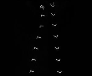
  $Re$ and motion direction over time. Two stable solutions are achieved for all three objects. The object tends to stabilize at approximately 1.5 s. All the results are in perfect agreement with the interpolation results based on the proposed approach (described later in § 4 in detail). The results obtained from the experiment were superimposed. The typical fall postures and trajectories are shown in figure 3(d). The snapshot intervals are 5, 3 and 4 frames for the elliptical, triangular and L-shaped objects, respectively. Therefore, the existence of multiple stable falling postures is demonstrated. The details are shown in Supplementary movie 1 is available at https://doi.org/10.1017/jfm.2024.557.

Figure 3. Experimental verification results of the multiple falling postures of the objects. (a–c) The variations in  $\theta _g$,
  $Re$ and
  $\theta _m$ over time for the elliptical, triangular and L-shaped objects released at different initial angles. (d) Results showing the fall postures and trajectories of the elliptical (left-hand), triangular (middle) and L-shaped (right-hand) objects.
4. Numerical simulation
4.1. Numerical methods
The two-dimensional Navier–Stokes equations governing the incompressible fluid flow are
 \begin{gather} \frac{\partial{u_i}}{\partial{x_i}}= 0, \end{gather}
 \begin{gather}\frac{\partial{u_i}}{\partial{t}}+u_j\frac{\partial{u_i}}{\partial{x_j}}={-}\frac{1}{\rho_f}\frac{\partial{p}}{\partial{x_i}}+ \nu\frac{\partial^2{u_i}}{\partial{x_j}\partial{x_j}}, \end{gather}
where  $i,j = 1, 2, p$ is the pressure. For clarity, the velocity components
  $u_1$ and
  $u_2$ are also denoted by
  $u_x$ and
  $u_y$, respectively. We use STAR-CCM+ software to solve these equations using the finite volume method. Here, a second-order upwind scheme is used to discretize the convective term, and steady and implicit unsteady solvers are used to perform transient calculations for stationary and falling objects, respectively. A six-degree-of-freedom motion solver is applied to simulate the migration of an object under flow-induced forces as well as gravity.
A rectangular computational domain is adopted, and the size of the domain is large enough to eliminate the boundary effect. Since the dimensions and shapes of the objects are different, the computational domain sizes used here are different for different shapes. The distances from the upstream, downstream and lateral boundaries to the centre of the object are no less than  $49d$,
  $149d$ and
  $62d$, respectively. For the numerical simulation of the falling object, a moving computing domain is adopted based on the overset grid method. The computational domain moves at the same speed as the object. This approach ensures a sufficiently long development process for simulating the falling object. The overset mesh scheme is employed to solve the problem of rotational and large amplitude horizontal migration of an object during its fall.
In order to verify the accuracy of the calculations, the numerical simulation results for the fixed ellipse were verified. Table 1 is a comparison of  $C_D$,
  $C_L$ and
  $C_M$ for fixed ellipses between the present numerical simulations and the literature. Drag coefficient
  $C_D$ and lift coefficient
  $C_L$ are
 \begin{gather} {C_D}= \frac{2F_D}{\rho_fU_r^{2}d}, \end{gather}
 \begin{gather}{C_L}= \frac{2F_L}{\rho_fU_r^{2}d}, \end{gather}
where  $F_L$ and
  $F_D$ are lift and drag. The results at different Reynolds numbers are in good agreement with the literature. In numerical simulations, the computational domain is partitioned into a set of unstructured trimmed cells. The mesh is initially generated at a basic size, it is refined in the region containing the object. The effects of the grid resolution on the calculated results are verified for the elliptical object using four meshes with different numbers of elements from 51 670 to 105 211. As shown in table 2, good agreement is obtained for the cases with different meshes, indicating good grid convergence. In the simulation of this work, we all use the M2 which is shown in figure 4. Here M2 is used for all the following simulations in this study.
Table 1. Comparison of results for  $C_D$,
  $C_L$ and
  $C_M$ for
  $Re=15$ and 30 (the characteristic length is the length of the major axis of the ellipse),
  $\alpha =45$.

Table 2. Effect of the mesh resolution of the ellipse on the drag coefficient  $C_D$ when
  $Re = 25$ (the characteristic length is the length of the major axis of the ellipse), and
  $\alpha =90$.


Figure 4. Grid distribution of ellipse in a falling view. (a) The mesh in the whole computational domain. (b) Close-up view of the mesh around the object.
4.2. Interpolated results
As in the experiments, we consider elliptical, triangular and L-shaped objects as shown in figure 2(b–d). Based on the extensive numerical simulations for flow past the fixed objects, the fluid force and moment for the objects at different  $Re$ and
  $\alpha$ are obtained. The
  $Re$ ranges from 1 to 15 at an interval of 0.5 or 1, while
  $\alpha$ ranges from
  $0^\circ$ to
  $360^\circ$ at an interval of
  $10^\circ$. Figure 5 shows the distribution of the CoG lines for elliptical, triangular and L-shaped objects, respectively, at
  $Ar = 150$ and
  $m^* = 0.5$. For each shape, the stable solutions of the CoG line are depicted for the incidence angle
  $\alpha$, ranging from
  $0^\circ$ to
  $360^\circ$ at an interval of
  $10^\circ$. The solution map for each shape can be classified into several base families according to the distribution. Figure 5(a) illustrates two base families of CoG lines for an elliptical object, denoted in yellow (family 1) and blue (family 2), respectively. Each base family of solution is of a trumpet shape with its mouth facing outward and the tip facing inward. Therefore, in regions where different base families overlap, the CoG lines intersect, indicating the existence of multiple stable falling solutions. The overlapped multiple-solution region is represented in figure 5(b) using a mixed colour (green) of the base family colours (blue and yellow). A similar procedure is employed for the more complex cases with additional base families. As shown in figure 5(c–e), a pink colour is introduced to represent a third base family. The dark brown area represents the convergence of three base families, indicating that three different falling postures can occur there. These regions are named as SS fall posture regions, BS fall posture regions and TS fall posture regions, respectively. As shown in these figures, the ellipse has no more than two stable falling postures. However, up to three stable solutions can be obtained for the triangular and L-shaped objects. It is noted that the single-solution area still dominates the majority of the map.

Figure 5. Distribution of CoG lines for elliptical, triangular and L-shaped objects at  $Ar = 150$ and
  $m^* = 0.5$. (a) Two base families of CoG lines of elliptical objects. (b) The single stable (SS) fall posture region and bistable (BS) fall postures region of elliptical. (c) Three base families of CoG lines of triangle objects. (d,e) The SS, BS and tristable (TS) fall postures regions of (d) triangular and (e) L-shaped objects.
4.3. Parameter influence
In the methodology for determining stable postures, it is found that the direction of the CoG line is only determined by  $Ar$. This is because the direction of the CoG line is dependent on the direction of the force on the object, and the direction of the force on a fixed object is determined by the angle of attack and the
  $Re$ together. The
  $Re$ is embodied in
  $Ar$, so the direction of the CoG line at a certain angle of attack is determined by
  $Ar$. The magnitude of
  $L$ is determined by
  $m^*$,
  $C_F$ and
  $C_M$, where
  $C_F$ and
  $C_M$ are also determined by
  $Ar$ in the same way as the direction of the CoG line. Therefore, the distance
  $L$ of the CoG line from the origin is determined by
  $m^*$ and
  $Ar$ together.
Figure 6(a) shows the distribution of the boundary of the different regions under different  $m^*$ when
  $Ar=100$. The force and the moment coefficient on a stationary object remain constant when
  $Ar$ is constant, thus, the relationship between
  $L$ and
  $m^*$ is linear. The entire boundary is enlarged by a corresponding factor centred on the coordinate origin as
  $m^*$ increases. Therefore, the area of the BS and TS region is linear with
  ${m^*}^2$. Figure 6(b) shows the boundary distribution between different regions under different
  $Ar$ when
  $m^*=0.5$. When
  $m^*$ is constant, the area of the BS and TS region increases with the increase of
  $Ar$. To the extent that the force on the fixed objects is stabilized,
  $Ar$ has less effect on the distribution in the SS, BS and TS region which is due to the small variation of forces and moments on fixed objects over a small range of
  $Re$.
$Re$.

Figure 6. The influence of  $Ar$ and
  $m^*$ on the boundary of SS, BS and TS region. (a) The boundary of SS, BS and TS region changes with
  $m^*$ when
  $Ar = 100$. (b) The boundary of the SS, BS and TS region changes with
  $Ar$ when
  $m^* = 0.5$.
4.4. Free-fall tests
The experiment faced limitations due to material selection and manufacturing accuracy. To ensure that the geometric centre is positioned within the multisolution region, copper was selected as the material for the object, resulting in  $m^*$ being greater than 0.8. In contrast, the convenience of numerical computation allows for the selection of appropriate parameters to discover three stable falling postures. Therefore, the free-falling simulation is conducted for the cases at
  $Ar = 150$ and
  $m^* = 0.5$. As shown in figure 7(a), three shapes same to the experiments, i.e. the ellipse, triangle and L-shape, are considered, and the coordinates of their CoGs (CoG1, CoG2 and CoG3) that are listed in table 3 are selected in SS, BS and TS regions. For the initial state of a falling object, parameters such as initial velocity, angular velocity and initial release angle are considered. In this study, the object is released from a state of rest, so the initial state is characterized solely by the initial release angle. Therefore, 12 independent free-falls are simulated at different initial angles with an interval of 30
 $^\circ$ for each object. Figures 7(b) and 8 show the variations in the gravity direction,
  $Re$ and motion direction over time. All the terminal stable falling postures perfectly coincide with interpolation results based on the proposed method, confirming the existence of multiple stable falling postures.
Table 3. The dimensionless coordinates of CoG for the objects selected in numerical simulations.


Figure 7. Numerical verification of the multiple falling postures of the objects. (a) The selected CoGs in different regions and the  $\theta _g$ obtained by the proposed method of these CoGs. (b) The change in gravity direction with time for selected CoGs released at various initial angles and the potential energy of the chosen CoGs at different
  $\theta _g$ of (i) elliptical, (ii) triangular and (iii) L-shaped objects when
  $Ar = 150$ and
  $m^* = 0.5$.

Figure 8. The change in  $Re$ (a) and
  $\theta _m$ (b) with time for selected CoGs released at various initial angles of elliptical (i), triangular (ii) and L-shaped (iii) objects when
  $Ar = 150$ and
  $m^* = 0.5$.
In terms of the potential energy, a multiple stable system has multiple local minimums corresponding to the static stable equilibrium solutions and local maximums corresponding to the unstable equilibrium solutions. Here, we define the potential energy as
 \begin{equation} {E}={-}\int_{0}^{\theta_g}N\, {\rm d} \theta, \end{equation}
where  $N$ represents the restoring moment caused by gravity at
  $\theta _g$. Specifically,
  $N=Gd'$, where
  $d'$ is the distance from the CoG of the object to the CoG line at
  $\theta _g$. As shown in figure 7(b), the number and locations of potential wells agree well with those of the interpolation results based on the proposed method. The deeper the potential well corresponds the more easily attainable falling posture. It also corresponds to a wider range of initial release angles. Therefore, it is concluded that the proposed method based on the static flow simulation can interpolate to obtain the stable posture solution of the free-falling body in fluid at low
  $Re$.
$Re$.
4.5. Discussions on general shapes
Figure 9 shows the stabilized falling posture maps obtained by interpolation with the proposed method at  $Ar=150$ and
  $m^*=0.9$. This analysis reveals the shape dependence of the stability solution distribution. The maximum number of solutions for a square triangle, a square and an equilateral pentagon are three, four and five, respectively. It appears that, for equilateral shapes, the maximum number of solutions for a given object equals the number of its edges. However, this does not mean that the existence of multiple solutions is due to the rotational symmetry features of the objects. In addition, there is a correlation between the increase in the number of sides of the shape and the decrease in the area of the multiple solution area. Shapes resembling an equilateral form, such as the cross and H-shape illustrated in figures 9(e) and 9(f), tend to show a maximum number of solutions similar to that of a square. The distribution of these CoG lines is categorized into several ‘trumpet’ shapes, as shown in figure 9. It is observed that the primary dimension of the object, either the longest edge or the maximum projected dimension, significantly influences these trumpet distributions. Each primary dimension corresponds to a trumpet with the deepest tip. For instance, the trumpet distribution for a square aligns with its four edges, whereas for a rhombus, it aligns with its maximum projected dimension. Shorter sides may also have corresponding trumpets, as shown in the upper side of the T-shaped trumpet in figure 9(g). The presence of concavity in a shape tends to enhance the formation and depth of these trumpets, leading to a larger area of multiple solutions. This is evident in the cross-shaped, H-shaped, T-shaped and U-shaped objects. Conversely, convex features tend to have the opposite effect, as observed in the distribution diagram of the U-shaped object in figure 9(h).

Figure 9. Solution maps for the equilateral triangle (a), square (b), equilateral pentagon (c), rhombus (d), cross (e), H-shape (f), T-shape (g) and U-shape (h) at  $Ar = 150$ and
  $m^* = 0.9$.
5. Conclusions
Based on the above studies, it is concluded that an object with specific properties may have multiple stable falling postures at low Reynolds numbers. This discovery highlights the existence of multiple stable solutions that are universally present across objects of different shapes. The method proposed in this work can efficiently obtain results for the full parameter domain of an object. This saves computational cost and provides a clearer view of the results. Moreover, this methodology can also guide subsequent work on the study of objects falling. This method is also applicable to three-dimensional objects, by adding an extra dimension to the computation for fixed objects. Given that the computational coefficient for fixed objects is higher than that for the falling of three-dimensional objects, employing this method is a preferred means of saving computational cost. However, the increase in the number of dimensions results in a significant increase in the number of computational angles and computational cost. Additionally, handling and visualizing the CoG line of three-dimensional objects becomes somewhat more challenging. The implications of this research can be extended to the design, stability control and trajectory prediction for free and controlled flights in both air and water.
Supplementary movie
Supplementary movie is available at https://doi.org/10.1017/jfm.2024.557.
Acknowledgements
The authors are grateful to Professor L. Zhao for the helpful discussions.
Funding
This work is supported by the National Key Research and Development Plan (grant no. 2023YFC3107404) and National Natural Science Foundation of China (grant nos. 52422110, U20A20328).
Declaration of interests
The authors report no conflict of interest.


