3.1. Examinations of local isotropy

Near the wall, the flow is highly anisotropic due to wall effects, the flow quantities are sensitive to the boundary conditions and thus the universality of small-scale quantities can hardly be observed. Therefore, examining the results in the locally isotropic region is effective for evaluating the universality of statistics in the presence of the real-fluid effects since the wall effects have been largely eliminated. We begin with examining the validity of local isotropy of small-scale statistics. Provided that the flow is locally isotropic, the even moments of velocity gradient should obey the following relations (Taylor Reference Taylor1935; Jiang et al. Reference Jiang, Hu, Cheng and Zhou2022):

(3.1)\begin{equation}\overline {{{\left( {\frac{{\partial u^{\prime}}}{{\partial x}}} \right)}^2}} = \overline {{{\left( {\frac{{\partial v^{\prime}}}{{\partial y}}} \right)}^2}} = \overline {{{\left( {\frac{{\partial w^{\prime}}}{{\partial z}}} \right)}^2}} = \frac{1}{2}\overline {{{\left( {\frac{{\partial {u^{\prime}_i}}}{{\partial {x_j}}}} \right)}^2}} ,\end{equation}

with i ≠ j and no summation on i and j. Thus, the local isotropy of the second-order moments of velocity gradients indicates

(3.2a)\begin{gather}{A_1} = {{\overline {{{\left( {\frac{{\partial u^{\prime}}}{{\partial x}}} \right)}^2}} } / {\overline {{{\left( {\frac{{\partial v^{\prime}}}{{\partial y}}} \right)}^2}} }} = 1,\quad {A_2} = {{\overline {{{\left( {\frac{{\partial u^{\prime}}}{{\partial x}}} \right)}^2}} } / {\overline {{{\left( {\frac{{\partial w^{\prime}}}{{\partial z}}} \right)}^2}} }} = 1,\end{gather}

(3.2b)\begin{gather}{A_3} = 2{{\overline {{{\left( {\frac{{\partial u^{\prime}}}{{\partial x}}} \right)}^2}} } / {\overline {{{\left( {\frac{{\partial u^{\prime}}}{{\partial y}}} \right)}^2}} }} = 1,\quad {A_4} = 2{{\overline {{{\left( {\frac{{\partial u^{\prime}}}{{\partial x}}} \right)}^2}} } / {\overline {{{\left( {\frac{{\partial u^{\prime}}}{{\partial z}}} \right)}^2}} }} = 1,\end{gather}

(3.2c)\begin{gather}{A_5} = 2{{\overline {{{\left( {\frac{{\partial u^{\prime}}}{{\partial x}}} \right)}^2}} } / {\overline {{{\left( {\frac{{\partial v^{\prime}}}{{\partial x}}} \right)}^2}} }} = 1,\quad {A_6} = 2{{\overline {{{\left( {\frac{{\partial u^{\prime}}}{{\partial x}}} \right)}^2}} } / {\overline {{{\left( {\frac{{\partial v^{\prime}}}{{\partial z}}} \right)}^2}} }} = 1,\end{gather}

(3.2d)\begin{gather}{A_7} = 2{{\overline {{{\left( {\frac{{\partial u^{\prime}}}{{\partial x}}} \right)}^2}} } / {\overline {{{\left( {\frac{{\partial w^{\prime}}}{{\partial x}}} \right)}^2}} }} = 1,\quad {A_8} = 2{{\overline {{{\left( {\frac{{\partial u^{\prime}}}{{\partial x}}} \right)}^2}} } / {\overline {{{\left( {\frac{{\partial w^{\prime}}}{{\partial y}}} \right)}^2}} }} = 1.\end{gather}

According to Tang et al. (Reference Tang, Antonia, A, Djenidi, Abe, Zhou, Danaila and Zhou2015), the local isotropy of the third-order and fourth-order moments of the velocity gradient leads to

(3.3)\begin{gather}{S_{\partial u^{\prime}/\partial x}} = {S_{\partial v^{\prime}/\partial y}} = {S_{\partial w^{\prime}/\partial z}},\end{gather}

(3.4)\begin{gather}{F_{\partial u^{\prime}/\partial x}} = {F_{\partial v^{\prime}/\partial y}} = {F_{\partial w^{\prime}/\partial z}}.\end{gather}

Figure 2 examines the local isotropy of the small-scale statistics along the wall-normal direction. In figure 2(a), we show the Lumley triangle, which examines the non-zero invariants I ₁ and I ₂ of the anisotropic part of the Reynolds stress tensor ${a_{ij}} = \overline {{u^{\prime}_i}{u^{\prime}_j}} /\overline {{u^{\prime}_k}{u^{\prime}_k}} - {\delta _{ij}}/3$, with ${I_1} = \sqrt {{a_{ij}}{a_{ji}}/6}$ and ${I_2} = {(1/6{a_{ij}}{a_{jk}}{a_{ki}})^{1/3}}$. As in Lumley & Newman (Reference Lumley and Newman1977), the triangle corresponds to I ₁ = I ₂, I ₁ = −I ₂ and ${I_1} = \sqrt {2I_2^3 + 1/27}$. As the distance to the wall increases, the variants approach I ₁ = 0 and I ₂ = 0 which corresponds to the isotropic condition, as indicated by the arrow, implying that the departure from isotropy becomes smaller. Figure 2(b) shows the wall-normal distribution of A_i for TR3. The results confirm that at 0.3 < ζ/L_y < 1 near both walls, A_i shows a gradual convergence towards unity and lies within the ±20 % boundaries of local isotropy (indicated by the dashed lines), which suggests that the local isotropy hypothesis within this wall-normal range (0.3 < ζ/L_y < 1) is approximately valid. The results for other cases are similar to those of TR3 and are not shown here for brevity. Figure 2(c) shows the skewness of the velocity gradient components according to (3.3). It can be seen that at ζ/L_y > 0.25 near both walls, all distributions exhibit a region where the magnitudes of the velocity-derivative skewness are approximately consistent. Figure 2(d) compares the distributions of ${F_{\partial u^{\prime}/\partial x}}$, ${F_{\partial v^{\prime}/\partial y}}$ and ${F_{\partial w^{\prime}/\partial z}}$, showing that the local isotropy condition (3.4) is satisfied reasonably well when ζ/L_y > 0.3. Thus, we can determine the ζ/L_y range of locally isotropic region as 0.3 < ζ/L_y < 1 near both walls. According to this, table 2 shows ζ/L_y, ζ ⁺ and ζ* of the start point of the locally isotropic region (LIR) of the channel for all cases.

Table 2. Here, ζ/L_y, ζ ⁺ and ζ* of the start point of the locally isotropic region for all cases, where ${\zeta ^ + } = \sqrt {{\rho _w}{\tau _w}} \zeta /{\mu _w}$ and ${\zeta ^\ast } = \sqrt {\bar{\rho }{\tau _w}} \zeta /\bar{\mu }$ are wall units and semilocal wall units, respectively, and ${\tau _w}$ is the wall shear stress.

3.2. Small-scale universality: velocity gradients and dissipation rate

Figure 3 shows PDFs of the longitudinal two-point velocity increments $\mathrm{\Delta }u^{\prime} = u^{\prime}(x + r,y,z) - u^{\prime}(x,y,z)$ at different wall-normal positions for all cases. We find that the PDFs of the longitudinal velocity increments pass through a transition from super-Gaussian to nearly Gaussian (or slightly sub-Gaussian) behaviour as the two-point distance increases (see figure 3a–d), suggesting intermittency at the small scales. In figure 3(a), it can be seen that all PDF profiles are quite consistent; although the PDFs are close to exponential decay, there are still slight discrepancies among all cases at the tail of the PDF profiles. In the following section, we will address the significance of these tails on the high-order moments of velocity gradients. In the near-wall layer (as shown in figure 3b), the discrepancies between different cases are more obvious, which is attributed to the anisotropic nature of the flow near the wall.

Figure 3. Profiles for PDFs of longitudinal velocity increments $\mathrm{\Delta }u^{\prime} = u^{\prime}(x + r,y,z) - u^{\prime}(x,y,z)$ near both walls for different cases: (a) r =Δx at ζ* = 300 in the LIR, where Δx is the streamwise grid spacing; (b) r =Δx at ζ* = 10; (c) r = 20Δx at ζ* = 300; (d) r = 100Δx at ζ* = 300. The x-axis is rescaled by the r.m.s. of velocity increments. The blue curves indicate cold wall profiles, the red curves correspond to hot wall profiles and black dashed lines denote the Gaussian distribution.

We display the PDFs of local dissipation scale r_d and local dissipation rate $\varepsilon /\bar{\varepsilon }$ near the cold wall and the hot wall in figure 4. The local dissipation scale, r_d, is determined such that $\bar{\rho }{(\mathrm{\Delta }u^{\prime})_{{r_d}}}{r_d}/\bar{\mu } = 1$ (Schumacher Reference Schumacher2007; Hamlington et al. Reference Hamlington, Krasnov, Boeck and Schumacher2012), with ${(\mathrm{\Delta }u^{\prime})_{{r_d}}}$ the streamwise velocity-fluctuation increments over the streamwise distance r_d. Thus, the PDFs of local dissipation scale can formally be written as $P[{r_d}|0.9 \le \bar{\rho }{(\mathrm{\Delta }u^{\prime})_{{r_d}}}r/\bar{\mu } \le 1.1]$ (Hamlington et al. Reference Hamlington, Krasnov, Boeck and Schumacher2012). It should be noted that the Kolmogorov scale, $\bar{\eta } = {[{(\bar{\mu }/\bar{\rho })^3}\bar{\rho }/\bar{\varepsilon }]^{1/4}}$, only results from the dimensional analysis and may contain the length scales at the dissipative range and the inertial range. According to Hamlington et al. (Reference Hamlington, Krasnov, Boeck and Schumacher2012), including only values of r_d in the above definition of local dissipation scale can ensure the isolation of the flow structures occurring at the cutoff of dissipative range and inertial range. Knowledge of the PDFs of the local dissipation scales, given in figure 4, provides evidence of the similarity of the characteristic length scale at the dissipative range for transcritical flows. Figure 4(a) shows $\textrm{PDF}({r_d})$ at ζ* = 300 for all cases. It can be seen that there are only small differences in $\textrm{PDF}({r_d}/\overline {{r_d}} )$ among cases, suggesting that $\textrm{PDF}({r_d}/\overline {{r_d}} )$ in the LIR of the channel is insensitive to the real-fluid variable-property effects. Similar observations can be made from figure 4(b), showing that the PDFs of dissipation rate, $\textrm{PDF}(\varepsilon /\bar{\varepsilon })$ approximately follows the log-normal distribution for $0.1 < \varepsilon /\bar{\varepsilon } < 2$, but deviates from the log-normal distribution for the extreme events at the tail. In the locally isotropic region, despite the different levels of density and viscosity fluctuations in the flows, the PDFs of the dissipation rate have similar profiles; our observations support the consistency of the local dissipation scale for transcritical cases.

Figure 4. The PDFs of (a) local dissipation scales and (b) dissipation rate in the LIR (at ${\zeta ^\ast } = 300$) of the channel for different cases: blue lines, cold wall profiles; red lines, hot wall profiles; black line, the log-normal fitting $\textrm{PD}{\textrm{F}_{\varepsilon /\bar{\varepsilon }}} = {y_0} + (A/(\sqrt {2{\rm \pi} } (\varepsilon /\bar{\varepsilon })\sigma ))\,\textrm{exp}[ - {(\textrm{ln}((\varepsilon /\bar{\varepsilon })/{x_c}))^2}/2{\sigma ^2}]$ with y ₀ = −0.00436, x_c = 0.682, σ = 1.232, A = 1.102.

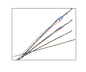
Results of the second-order structure function (S ₂) of $u^{\prime}$ for the LIR of the channel give similar insights into the small-scale flow structures. Figure 5 presents the longitudinal structure functions of fluctuating streamwise velocity ${S_2} = \overline {{{[u^{\prime}(x + r,y,z) - u^{\prime}(x,y,z)]}^2}}$ as a function of the streamwise spatial increment in the LIR of the channel for TR3. There is reasonable collapse of the distributions in the dissipative range with $r < 20\bar{\eta }$. In the LIR of the channel, the inertial region of S ₂ normalized by the mean dissipation rate (see figure 5a) and that normalized by the local dissipation rate (considering intermittency, see figure 5b) have not yet been observed in either case due to the Reynolds number not being sufficiently large. In the dissipative range, according to Kolmogorov's first similarity hypothesis, the viscosity and dissipation rate dominate the structure function. A simple dimensional analysis yields the expression of the second-order structure function

(3.5)\begin{equation}{S_2} = {C_2}\left( {\frac{{\bar{\rho }{{\bar{\varepsilon }}_0}}}{{\bar{\mu }}}} \right){r^2},\end{equation}

with C ₂ the second-order structure function coefficient, and ${\varepsilon _0} = \varepsilon /\rho$. Equation (3.5) indicates that the second-order structure function for transcritical flows is consistent with that of the incompressible flows given in Pope (Reference Pope2000). In summary, despite the small discrepancies at the tail of the $\partial u^{\prime}/\partial x$-PDF profiles, the low-order structure functions of $u^{\prime}$ for all cases have the same scaling in the dissipative range.

Figure 5. Second-order structure functions of $u^{\prime}$ (${S_2} = \overline {{{[u^{\prime}(x + r,y,z) - u^{\prime}(x,y,z)]}^2}}$) as a function of streamwise spatial increment in the LIR of the channel for TR3: (a) S ₂ rescaled by the mean dissipation rate ${\bar{\varepsilon }_0}$; (b) S ₂ rescaled by local dissipation rate (ε ₀ averaged over the streamwise two-point distance).

3.3. Real-fluid effects on moments of small-scale statistics

The moments of the velocity gradients and dissipation rate play an important role for characterizing the small-scale dynamics. The nth-order moments of turbulent statistics can be written as

(3.6)\begin{equation}{M_n}(Z) = \frac{{\overline {{Z^n}} }}{{{{(\overline {{Z^2}} )}^{n/2}}}},\end{equation}

with Z denoting any flow quantity. Figure 6(a,b) shows the variations of the skewness of the velocity gradient ($Z = \partial u^{\prime}/\partial x$, n = 3 in (3.6)) and the flatness of the velocity gradient ($Z = \partial u^{\prime}/\partial x$, n = 4 in (3.6)) as a function of ζ* for all cases. It can be seen that ${M_3}(\partial u^{\prime}/\partial x)$ (i.e. ${S_{\partial u^{\prime}/\partial x}}$) and ${M_4}(\partial u^{\prime}/\partial x)$ (i.e. ${F_{\partial u^{\prime}/\partial x}}$) away from the wall are nearly constant. Distributions of ${S_{\partial u^{\prime}/\partial x}}$ or ${F_{\partial u^{\prime}/\partial x}}$ are qualitatively similar for all the wall flows, with minor quantitative variations. As the distance to the wall increases, ${S_{\partial u^{\prime}/\partial x}}$ decreases, reaches a minimum, increases and finally forms a plateau in the outer region of the flow. This behaviour is also consistent with that of incompressible flows with moderate and high Re_τ reported in Djenidi et al. (Reference Djenidi, Antonia, Talluru and Abe2017). We can also observe the characteristic behaviour of ${F_{\partial u^{\prime}/\partial x}}$ for all transcritical cases, it is found that ${F_{\partial u^{\prime}/\partial x}}$ approaches a constant, which is independent of the thermal property changes. In Appendix C, we examine the results based on density-weighted velocity fluctuations, and confirm that the results of density-weighted velocity-fluctuation derivatives are consistent with the Reynolds-averaged results.

Figure 6. Moments of fluctuating streamwise velocity gradients (see (3.6)) in different cases: (a) $Z = \partial u^{\prime}/\partial x$, n = 3 (skewness) as a function of ζ*; (b) $Z = \partial u^{\prime}/\partial x$, n = 4 (flatness) as a function of ζ*; (c) $Z = \partial u^{\prime}/\partial x$, n = 3 (skewness) as a function of semilocal Taylor Reynolds number $Re_\lambda ^\ast $; (d) $Z = \partial u^{\prime}/\partial x$, n = 4 (flatness) as a function of $Re_\lambda ^\ast $. In (c) and (d), open symbols represent the results in the LIR of the channel whereas solid symbols indicate the near-wall layers; blue, near the cold wall for TR3; red, near the hot wall for TR3; black, near the cold wall for TR1.9; pink, near the hot wall for TR1.9; purple, near the cold wall for TR1.4; green, near the hot wall for TR1.4; grey, TR1.

We make two additional remarks here. First, the data from Abe, Antonia & Kawamura (Reference Abe, Antonia and Kawamura2009) showed that the plateau of the velocity gradient skewness did not occur for Re_τ = 180, while this plateau can be clearly observed in the LIR of the channel when Re_τ reaches 590 for incompressible flows (Vreman & Kuerten, Reference Vreman and Kuerten2014). Our results also indicate that at transcritical conditions, the plateau where ${S_{\partial u^{\prime}/\partial x}}$ and ${F_{\partial u^{\prime}/\partial x}}$ remain constant definitely exists when Re_τ exceeds 300 (i.e. the lowest Re_τ in the present study); this supports that ${S_{\partial u^{\prime}/\partial x}}$ and ${F_{\partial u^{\prime}/\partial x}}$ in the LIR of the channel are independent of ζ* when Re_τ exceeds 300, which is approximately consistent with the Re_τ threshold for ${S_{\partial u^{\prime}/\partial x}} = \textrm{const}\textrm{.}$ and ${F_{\partial u^{\prime}/\partial x}} = \textrm{const}\textrm{.}$ for incompressible turbulence. Second, in the LIR of the channel, the level of agreement of ${S_{\partial u^{\prime}/\partial x}}$ and ${F_{\partial u^{\prime}/\partial x}}$ between the present study and the previous studies on incompressible channel flows (Abe et al. Reference Abe, Antonia and Kawamura2009; Vreman & Kuerten Reference Vreman and Kuerten2014; Tang et al. Reference Tang, Antonia, A, Djenidi, Abe, Zhou, Danaila and Zhou2015; Antonia et al. Reference Antonia, Djenidi, Danaila and Tang2017; Tang et al. Reference Tang, Antonia, Djenidi and Zhou2019) is relatively poor. Abe et al. (Reference Abe, Antonia and Kawamura2009) reported that ${S_{\partial u^{\prime}/\partial x}} ={-} 0.6$ in the outer layer for Re_τ = 395 and 640 (comparable magnitude with the present study) while ${S_{\partial u^{\prime}/\partial x}}$ remains less than −0.5 according to Vreman & Kuerten (Reference Vreman and Kuerten2014). Xu, Antonia & Rajagopalan (Reference Xu, Antonia and Rajagopalan2001) found that ${S_{\partial u^{\prime}/\partial x}}$ and ${F_{\partial u^{\prime}/\partial x}}$ remain −0.53 and 10 at Re_λ > 200–300 in the outer layer of incompressible plane jet and circular jet. The current transcritical cases suggest that ${S_{\partial u^{\prime}/\partial x}}$ and ${F_{\partial u^{\prime}/\partial x}}$ converge at similar Re_τ and Re_λ compared with incompressible flows (i.e. Re_τ = 300–600 or Re_λ = 200–300). However, the corresponding values of the ${S_{\partial u^{\prime}/\partial x}}$ and ${F_{\partial u^{\prime}/\partial x}}$ plateau (${S_{\partial u^{\prime}/\partial x}} ={-} 0.25$ and ${F_{\partial u^{\prime}/\partial x}} = 4$) are different from those of incompressible flows, which means that the discrepancies between transcritical flows and incompressible flows are mainly associated with the effects of real-fluid property variations, while the Reynolds number effect contributes only minimally. Note that even for TR1 for which the two walls have the same temperature and heat, transfer is weak, although the boundary condition is similar to that of incompressible flows, the small-scale statistics still differ from the incompressible flows. The small pressure fluctuations in the flow also lead to large thermal property changes, leading to $Re_\lambda ^\ast $ varying from 700 at the wall to 1000 at the centreline and thus turbulence dynamics depart significantly from incompressible flows. This may explain the differences of the ${S_{\partial u^{\prime}/\partial x}}$ and ${F_{\partial u^{\prime}/\partial x}}$ profiles between TR1 and incompressible flows studied in the prior studies (Abe et al. Reference Abe, Antonia and Kawamura2009; Vreman & Kuerten Reference Vreman and Kuerten2014; Tang et al. Reference Tang, Antonia, A, Djenidi, Abe, Zhou, Danaila and Zhou2015; Antonia et al. Reference Antonia, Djenidi, Danaila and Tang2017; Tang et al. Reference Tang, Antonia, Djenidi and Zhou2019).

Next we assess the behaviour of ${S_{\partial u^{\prime}/\partial x}}$ and ${F_{\partial u^{\prime}/\partial x}}$ in terms of Taylor Reynolds number (see figure 6c,d; $Re_\lambda ^\ast= \bar{\rho }u^{\prime}\lambda /\bar{\mu }$ is semilocal Taylor Reynolds number defined based on the local density and viscosity along the wall-normal direction). In the context of K41 (Kolmogorov Reference Kolmogorov1941), both S and F in incompressible flows are approximately independent of Re_λ; whereas in K62 (Kolmogorov Reference Kolmogorov1962; Obukhov Reference Obukhov1962), S and F are expected to increase with increasing Re_λ. To clearly distinguish the profiles in the LIR of the channel, we use different symbols to identify different wall-normal positions in the channels. Figure 6(c,d) shows that the universality of skewness and flatness of fluctuating streamwise velocity gradients with $Re_\lambda ^\ast $ in the locally isotropic region (see the open symbols) manifests primarily. Moreover, in all cases, ${S_{\partial u^{\prime}/\partial x}}$ in the LIR is nearly independent of $Re_\lambda ^\ast $, providing support for K41 at transcritical conditions; ${S_{\partial u^{\prime}/\partial x}}$ becomes constant when $Re_\lambda ^\ast \; > 150$ (as shown in figure 6c). These conclusions bear analogies with those for incompressible flows in which ${S_{\partial u^{\prime}/\partial x}}$ becomes independent of $R{e_\lambda }$ when $R{e_\lambda }\; > 100$ for jet flows (Tang et al. Reference Tang, Antonia, Djenidi and Zhou2019) and when $R{e_\lambda } > 150$ for wall-bounded flows (Djenidi et al. Reference Djenidi, Antonia, Talluru and Abe2017) (note that $R{e_\lambda } \equiv Re_\lambda ^\ast $ for incompressible flows). With regard to ${F_{\partial u^{\prime}/\partial x}}$, we find that in the LIR of the channel for transcritical flows, ${F_{\partial u^{\prime}/\partial x}}$ remains approximately constant for $100 < Re_\lambda ^\ast \; < 300$ (see the open symbols in figure 6d). For incompressible flows, results of isotropic flows and jet flows (van Atta & Antonia Reference Van Atta and Antonia1980; Kerr Reference Kerr1985; Sreenivasan & Antonia Reference Sreenivasan and Antonia1997) show that ${F_{\partial u^{\prime}/\partial x}}$ varies slightly with $R{e_\lambda }$ when $R{e_\lambda }\; < 100$, and then increases monotonically with $R{e_\lambda }$ for $R{e_\lambda } \in ({10^2},{10^3})$. However, Djenidi et al. (Reference Djenidi, Antonia, Talluru and Abe2017) pointed out that the plateau of F occurs when $R{e_\lambda }$ reaches 100–500 in wall-bounded flows. According to the above discussions, ${F_{\partial u^{\prime}/\partial x}}$ for transcritical wall-bounded flows also exhibits consistency with the incompressible wall flows.

According to K41 and K62, the consistency of the small-scale statistics for incompressible cases is only valid for sufficiently large Reynolds numbers. From the results of figures 3–6, we conclude that the moments of the velocity gradients with order n ≤ 4 follow the universal behaviours (thought to exist only at very high Reynolds numbers) in the presence of real-fluid thermodynamic property variations even at relatively moderate Reynolds numbers.

In figure 7, we show the moments of the local dissipation rate $\overline {{\varepsilon ^n}} /{\bar{\varepsilon }^n}$ as a function of ζ* in the LIR for transcritical channel flows. The dissipation moments $\overline {{\varepsilon ^n}} /{\bar{\varepsilon }^n}$ reflect the variations in the smallest dissipative scale, particularly for high n (Hamlington et al. Reference Hamlington, Krasnov, Boeck and Schumacher2012). Similar to the results for incompressible channel flows (Hamlington et al. Reference Hamlington, Krasnov, Boeck and Schumacher2012), the low-order moments of ε remain constant in the locally isotropic region (see figure 7a). In contrast, the high-order dissipation rate moments (n = 3) obey different behaviours (see figure 7b); the interesting point is that the high-order dissipation rate moments do not collapse in the LIR of the channel. The variable-property effects on high-order small-scale statistical moments will be elaborated on in the following section.

Figure 7. Variations of local dissipation rate moments $\overline {{\varepsilon ^n}} /{\bar{\varepsilon }^n}$ as functions of ζ* for different cases: (a) n = 2; (b) n = 3.

3.4. Real-fluid effects on small-scale high-order statistical moments

Our analysis shows that low-order moments of small-scale statistics such as dissipative length scale, dissipation rate and the velocity gradient have universal behaviours at transcritical conditions. However, the high-order moments of small-scale statistics in transcritical flows are sensitive to real-fluid property variations. To clarify the modulations of these effects on the moments of velocity gradients and dissipation rate, we consider the following budget equation for local dissipation rate at transcritical conditions (Li et al. Reference Li, Guo, Bai and Ihme2023):

(3.7)\begin{align} \varepsilon & = \underbrace{{\bar{\mu }\dfrac{{\partial {u^{\prime}_i}}}{{\partial {x_j}}}\left( {\dfrac{{\partial {u^{\prime}_i}}}{{\partial {x_j}}} + \dfrac{{\partial {u^{\prime}_j}}}{{\partial {x_i}}}} \right)}}_{{{\varepsilon _I}}}\underbrace{{ - \dfrac{2}{3}\bar{\mu }{{(\boldsymbol{\nabla }\boldsymbol{\cdot }\boldsymbol{u^{\prime}})}^2}}}_{{{\varepsilon _{II}}}} \nonumber \\ & \quad + \underbrace{{\mu ^{\prime}\dfrac{{\partial {u^{\prime}_i}}}{{\partial {x_j}}}\left( {\dfrac{{\partial {{\bar{u}}_i}}}{{\partial {x_j}}} + \dfrac{{\partial {{\bar{u}}_j}}}{{\partial {x_i}}} - \dfrac{2}{3}\dfrac{{\partial {{\bar{u}}_k}}}{{\partial {x_k}}}{\delta_{ij}}} \right)}}_{{{\varepsilon _{III}}}} + \underbrace{{\dfrac{{\partial {u^{\prime}_i}}}{{\partial {x_j}}}\left[ {\mu^{\prime}\left( {\dfrac{{\partial {u^{\prime}_i}}}{{\partial {x_j}}} + \dfrac{{\partial {u^{\prime}_j}}}{{\partial {x_i}}} - \dfrac{2}{3}\dfrac{{\partial {u^{\prime}_k}}}{{\partial {x_k}}}{\delta_{ij}}} \right)} \right]}}_{{{\varepsilon _{IV}}}}, \end{align}

where ε_I is the solenoidal term composed of the mean viscosity and the enstrophy, ε_II denotes the dilatational term related to the fluctuating velocity divergence, ε_III and ε_IV are budgets related to the fluctuations of viscosity. In our previous study (Li et al. Reference Li, Guo, Bai and Ihme2023), we found that turbulent dissipation is dominated by the solenoidal term, which means that the dissipation rate is primarily generated by vorticity and the contributions from thermal property fluctuations are negligible. For incompressible flows, we can expect ε_II = ε_III = ε_IV = 0 and thus ε = ε_I. In the LIR of the channel, (3.1) is valid so that

(3.8)\begin{equation}\bar{\varepsilon } = 15\bar{\mu }\overline {{{\left( {\frac{{\partial u^{\prime}}}{{\partial x}}} \right)}^2}} .\end{equation}

According to (3.8), we can establish the relation between the dissipation rate moments and velocity gradient moments,

(3.9)\begin{equation}\frac{{\overline {{\varepsilon ^n}} }}{{{{\bar{\varepsilon }}^n}}} = \frac{{\overline {{{15}^n}{{\bar{\mu }}^n}{{\left( {\dfrac{{\partial u^{\prime}}}{{\partial x}}} \right)}^{2n}}} }}{{{{15}^n}{{\overline {\bar{\mu }{{\left( {\dfrac{{\partial u^{\prime}}}{{\partial x}}} \right)}^2}} }^n}}} = \frac{{\overline {{{\left( {\dfrac{{\partial u^{\prime}}}{{\partial x}}} \right)}^{2n}}} }}{{{{\overline {{{\left( {\dfrac{{\partial u^{\prime}}}{{\partial x}}} \right)}^2}} }^n}}} = {M_{2n}}\left( {\frac{{\partial u^{\prime}}}{{\partial x}}} \right).\end{equation}

Equations (3.9) shows that the skewness and flatness of velocity gradients are associated with the local dissipation rate moments in the LIR for channel flows. As discussed above, the PDFs of the longitudinal velocity gradient distribute similarly in the locally isotropic region of the channel, leading to the universal profiles of low-order dissipation rate moments, as shown in figure 7(a). However, as in Belin, Maurer & Willaime (Reference Belin, Maurer and Willaime1997), the discrepancy at the exponential-decaying low-probability tails can contribute significantly to high-order moments, resulting in the substantial discrepancies of high-order moments for different conditions. Figure 8 further shows the high-order structure functions. In figure 8(a), we first examine the profiles of the rescaled longitudinal structure function of the streamwise velocity ${S_{2n}}(r)/{r^{2n}}\;(n \le 4)$. The plateau of ${S_{2n}}(r)/{r^{2n}}$ at small-scale is visible, thus it follows ${S_{2n}}(r) \sim {r^{2n}}$ in the dissipative range. In light of the definition of ${S_{2n}}(r)$, we have the following relation in the dissipative range:

(3.10a,b)\begin{equation}\frac{{{S_2}}}{{{r^2}}} = \overline {{{\left( {\frac{{\partial u^{\prime}}}{{\partial x}}} \right)}^2}} ,\quad \frac{{{S_{2n}}}}{{{r^{2n}}}} = \overline {{{\left( {\frac{{\partial u^{\prime}}}{{\partial x}}} \right)}^{2n}}} ,\end{equation}

Figure 8. Variable-property effects on small-scale high-order statistics: (a) the longitudinal structure functions of the streamwise velocity ${S_{2n}}(r)/{r^{2n}} = \overline {{{(\mathrm{\Delta }u^{\prime})}^{2n}}} /{r^{2n}}\;(n \le 4)$ rescaled by ${({u_{\tau ,cold}}/{L_x})^{ - 2n}}$ at the channel centreline of TR3. The horizontal lines are defined by the converged value of the corresponding curves; (b) rescaled longitudinal structure function of the streamwise velocity ${S_{2n}}(r)/{(u_\tau ^\ast )^{2n}}$ at the channel centreline in TR1 (solid lines) and TR3 (dashed lines), with S _2n rescaled by $u_\tau ^\ast $ at the centreline of TR3; (c) PDFs of local dissipation rate moment ${\varepsilon ^2}/{\bar{\varepsilon }^2}$ at ζ* = 300 near the hot wall for all cases.

and thus,

(3.11)\begin{equation}{M_{2n}}\left( {\frac{{\partial u^{\prime}}}{{\partial x}}} \right) = \frac{{\overline {{{\left( {\dfrac{{\partial u^{\prime}}}{{\partial x}}} \right)}^{2n}}} }}{{{{\overline {{{\left( {\dfrac{{\partial u^{\prime}}}{{\partial x}}} \right)}^2}} }^n}}} = \frac{{{S_{2n}}}}{{S_2^n}} = \frac{{{C_{2n}}{{\left( {\dfrac{{\bar{\rho }\overline {{\varepsilon_0}} }}{{\bar{\mu }}}} \right)}^n}{r^{2n}}}}{{C_2^n{{\left( {\dfrac{{\bar{\rho }\overline {{\varepsilon_0}} }}{{\bar{\mu }}}} \right)}^n}{r^{2n}}}}.\end{equation}

Equation (3.11) yields

(3.12)\begin{equation}{M_{2n}}\left( {\frac{{\partial u^{\prime}}}{{\partial x}}} \right) = \frac{{{S_{2n}}}}{{S_2^n}} = \frac{{{C_{2n}}}}{{C_2^n}}.\end{equation}

Equation (3.11) indicates that the moments of the velocity gradient are determined by the structure functions in the dissipative range. Figure 8(b) gives the rescaled longitudinal structure function of the streamwise velocity ${S_{2n}}(r)/{(u_\tau ^\ast )^{2n}}$ at the channel centreline for TR1 and TR3. It is evident that as the order of the structure function (n) increases, the structure functions with the same order for different cases cannot collapse in the dissipative range, even though they still have the same scaling exponent with r. According to (3.12), the inconsistency of ${S_{2n}}/S_2^n$ between TR3 and TR1 indicates that the high-order structure function coefficient C _2n varies due to the variable-property effects in the channels (it is worth noting that in the context of incompressible turbulence, the structure function coefficient for a certain order is a constant), which essentially leads to the discrepancy of high-order moments of velocity gradient and dissipation rate in the LIR at transcritical conditions. Figure 8(c) shows PDFs of moments of local dissipation rate at ζ* = 300 near the hot wall for different cases. The PDFs of high-order dissipation rate for all cases cannot collapse, suggesting that the high-order moments of small-scale quantities are strongly sensitive to changes in thermal properties. Recalling that the PDF profiles of $\partial u^{\prime}/\partial x$ do not collapse at the tail, we expect that the rare events with high velocity gradients and turbulent dissipation contribute significantly to the discrepancies of high-order moments of dissipation rate between different cases.

3.5. Real-fluid effects on the scalings for small-scale statistics

This section examines the real-fluid effects on the scalings for small-scale statistics, including the structure function and dissipation rate moments. According to Kolmogorov's second hypothesis, S_n is independent of the viscosity in the inertial range (Kolmogorov Reference Kolmogorov1941; Pope Reference Pope2000), and hence dimensional analysis yields

(3.13)\begin{equation}{S_n}\sim {r^{{\zeta _n}}}.\end{equation}

Several models have been proposed for the intermittency factor ζ_n for locally isotropic flows at incompressible conditions, such as the refined similarity hypothesis (K62) (Kolmogorov Reference Kolmogorov1962; Obukhov Reference Obukhov1962),

(3.14)\begin{equation}{\zeta _n} = \frac{1}{3}n\left[ {1 - \frac{1}{6}\mu (n - 3)} \right],\quad \mu = 0.25,\end{equation}

and the universal scaling law (SL94) (She & Leveque Reference She and Leveque1994)

(3.15)\begin{equation}{\zeta _n} = \frac{n}{9} + 2\left[ {1 - {{\left( {\frac{2}{3}} \right)}^{n/3}}} \right].\end{equation}

Equations (3.14) and (3.15) were developed by considering the intermittency of the dissipation rate at high Reynolds number. Benzi et al. (Reference Benzi, Ciliberto, Tripiccione, Baudet, Massaioli and Succi1993) reported on the existence of an extended self-similarity (ESS) that holds for high and low Reynolds numbers, which is characterized by the universal scaling exponents of the structure functions with the independence of the Reynolds number. The ESS reads (Benzi et al. Reference Benzi, Ciliberto, Tripiccione, Baudet, Massaioli and Succi1993)

(3.16)\begin{equation}\overline {{{|{u^{\prime}(x + r,y,z) - u^{\prime}(x,y,z)} |}^n}} \propto {(|{{S_3}} |)^{{\zeta _n}}}.\end{equation}

Obviously $\overline {{{|{u^{\prime}(x + r,y,z) - u^{\prime}(x,y,z)} |}^n}} = {S_n}$ when n is even. Since the Re_τ and Re_λ considered in our study are relatively moderate, we use the ESS hypothesis to study the scaling for intermittency. Figure 9 shows plots of S ₂, S ₄, S ₆ and S ₈ as a function of the third-order structure function at the centreline for all conditions. For n = 2 and 4 (figure 9a,b), the results of all cases collapse onto a single profile which exhibits reasonably good agreement with the power law, even if no inertial range is established. Furthermore, self-similarity extends far beyond the inertial range deep into the dissipation range. We note that ζ_n in the LIR of the channel is insensitive to the wall-normal location (not shown here for brevity). These results show that the ESS exists at transcritical conditions for low-order structure functions. As n increases (see n = 6 and n = 8 shown in figure 9c,d), the profiles for S_n cannot collapse, suggesting that the ESS can hardly be applied for high-order structure functions and ζ_n becomes dependent on the real-fluid variable-property effects.

Figure 9. Plots of longitudinal structure functions of streamwise velocity (S ₂, S ₄, S ₆ and S ₈) as a function of |S ₃| at the centreline of the channel for all cases.

In table 3, we show the fitted value of ζ_n for n = 2–8 at transcritical conditions based on ESS, along with the coefficients of determination. The values of ζ_n are determined by fitting the data in the region of |S ₃| < 20, in which the structure functions closely follow the exponential law. The coefficients of determination (R ²) are higher than 0.99, implying the accuracy of the fitted results. To gain more insights into the real-fluid variable-property effects on the intermittency, we present ζ_n based on ESS computed for n = 2–8 at transcritical conditions in figure 10, with the predictions of ζ_n by K62 (Kolmogorov Reference Kolmogorov1962), SL94 (She & Leveque Reference She and Leveque1994) and incompressible ESS model (Benzi et al. Reference Benzi, Ciliberto, Tripiccione, Baudet, Massaioli and Succi1993) included. It is shown that ζ_n in the locally isotropic region of transcritical flows is higher than that of incompressible flows. Moreover, the noticeable difference is observed between ζ_n at transcritical conditions and that obtained by ESS for incompressible flow, implying again that the turbulent intermittency is largely affected by the real-fluid variable-property effects at transcritical conditions. Evidently, the modulations on intermittency are more significant for the higher-order structure functions.

Table 3. The fitted ζ_n based on ESS for n = 2–8 in all transcritical flows.

Figure 10. Scaling exponents ζ_n based on ESS computed for n = 2–8 at transcritical conditions for different cases. For comparison, the predictions of ζ_n by K62 (Kolmogorov Reference Kolmogorov1962), SL94 (She & Leveque Reference She and Leveque1994), incompressible ESS (Benzi et al. Reference Benzi, Ciliberto, Tripiccione, Baudet, Massaioli and Succi1993) and the experimental results of ζ_n in the locally isotropic flow for incompressible condition (the blue line, She & Leveque Reference She and Leveque1994) are also demonstrated.

The underlying mechanisms for intermittent behaviour are substantiated by means of visualizing the structures related to the rare events. Instantaneous isosurfaces of wall-normal velocity fluctuations as well as corresponding flooded contours of density in the locally isotropic region near the cold wall for TR1.9 and TR1.4 are shown in figure 11. The isosurfaces of wall-normal velocity fluctuations with $v^{\prime\prime} = 2.5$ m s⁻¹ and $v^{\prime\prime} = 1.2$ m s⁻¹ are associated with the rare structures with ρ > 680 kg m⁻³ for TR1.9, corresponding to the mean density value in the buffer layer. This implies clear ejection events from the near-wall layers as the near-wall turbulence lifts up the dense fluid in the buffer layer into the locally isotropic region with lower density. However, for TR1.4 with lower density ratio, such high-density rare structures from the near-wall layer are not obvious. This implies attenuated ejection motion of the rare structures with decreasing real-fluid thermodynamic effects in the channel. Evidently, these wall-normal coherent motions lead to significant mixing in the channel, resulting in effective momentum and energy transport between the near-wall layer and locally isotropic region. The comparison between the flow structures of TR1.9 and TR1.4 leads us to conclude that the ejection motions and turbulent mixing in the channel are enhanced as the increasing real-fluid effects. Since the ejected fluids from the near-wall layer have much lower density and tend to have higher velocity, their mixing with the core results in significant velocity increments in the locally isotropic layer and creates extreme events for high velocity gradients. This is a unique characteristic of transcritical wall-bounded flows which explains the extreme, rare events for high velocity gradients displayed in figure 3. Thus, the real-fluid variable-property effects play a first-order role in modulating the PDFs of higher-order structure functions and dissipation rate by introducing extreme, rare events for high velocity gradients; consequently, the higher-order structure function and its intermittency behave differently from those for incompressible flows.

Figure 11. Isosurfaces of wall-normal velocity fluctuation coloured by the instantaneous density in the locally isotropic region near the cold wall, with $v^{\prime\prime} = 1.2$ m s⁻¹ in (a,c) and $v^{\prime\prime} = 2.5$ m s⁻¹ in (b,d); here (a,b) TR1.9 and (c,d) TR1.4.

To provide more quantitative insights into the high-order moments of small-scale quantities, we compare the global Re dependence of local dissipation rate moments for different flows in figure 12. The global Re is defined as $Re = {\rho _w}U^{\prime}{L_y}/{\mu _w}$ with $U^{\prime}$ the r.m.s. of fluctuation velocity, $U^{\prime} = {\overline {({{u^{\prime}}^2} + {{v^{\prime}}^2} + {{w^{\prime}}^2})} ^{1/2}}$ and L_y the half-height of the channel (Hamlington et al. Reference Hamlington, Krasnov, Boeck and Schumacher2012; Schumacher et al. Reference Schumacher, Scheel, Krasnov, Donzis, Yakhot and Sreenivasan2014). Note that here the dissipation rate moments and Re are obtained by averaging the data over the whole LIR in the channel (Hamlington et al. Reference Hamlington, Krasnov, Boeck and Schumacher2012; Schumacher et al. Reference Schumacher, Scheel, Krasnov, Donzis, Yakhot and Sreenivasan2014). The scaling relation for the moments of the energy dissipation rate was derived from a theory for incompressible homogeneous and isotropic turbulence (Yakhot & Sreenivasan Reference Yakhot and Sreenivasan2005; Yakhot Reference Yakhot2006). It is given by

(3.17)\begin{equation}\overline {{\varepsilon ^n}} \propto R{e^{{d_n}}},\quad {d_n} = n + \frac{{{\theta _{4n}}}}{{{\theta _{4n}} - {\theta _{4n + 1}} - 1}}.\end{equation}

Figure 12. Scaling of dissipation rate moments against global Re for n = 2–4 in all cases (i.e. TR3 hot wall, TR3 cold wall, TR1.9 hot wall, TR1.9 cold wall, TR1.4 hot wall, TR1.4 cold wall and TR1). Here, $Re = {\rho _w}U^{\prime}{L_y}/{\mu _w}$ with $U^{\prime}$ the r.m.s. of fluctuation velocity, $U^{\prime} = {\overline {({{u^{\prime}}^2} + {{v^{\prime}}^2} + {{w^{\prime}}^2})} ^{1/2}}$ and L_y the half-height of the channel. The results of dissipation rate moments and Re are obtained by averaging the data within the whole LIR in the channel. Each symbol represents a separate flow case.

Here, θ_n is the inertial-range scaling exponent of the nth-order moment of the velocity increment $\mathrm{\Delta }u^{\prime}$. The error bar of 90 % confidence limits is also estimated and shown in figure 12 following a moving-block bootstrap method (Garcia, Jackson & Garcia Reference Garcia, Jackson and Garcia2005; Hamlington et al. Reference Hamlington, Krasnov, Boeck and Schumacher2012). The normalized dissipation moments are calculated in each snapshot over x–z planes, and the block sizes used to estimate the error bar are equal to one flow-through time, which is defined as ${L_x}/\overline {{u_b}}$ with $\overline {{u_b}}$ being the bulk velocity. The interesting point is that despite the different levels of density and viscosity fluctuations in the flows, the nth-order dissipation rate moments for all cases follow the same scaling law ($\overline {{\varepsilon ^n}} /{\bar{\varepsilon }^n}\sim R{e^{{d_n}}}$), strongly suggesting that the high-order energy dissipation statistics vary universally with Re at transcritical conditions. By fitting the scaling laws for each n (see dashed lines in figure 12), we find that the scaling exponents for the dissipation rate moments are d ₂ = 0.104, d ₃ = 0.622 and d ₄ = 1.237. Calculations of these exponents for incompressible homogeneously isotropic turbulence were shown to give d ₂ = 0.152, d ₃ = 0.476 and d ₄ = 0.978 (Yakhot Reference Yakhot2006; Schumacher Reference Schumacher2007); Hamlington et al. (Reference Hamlington, Krasnov, Boeck and Schumacher2012) reported that the local dissipation rate for incompressible channel flows follows the same scaling as that for isotropic flows. Our results show that although the dissipation rate moments at transcritical conditions collapse to the same scaling, the scaling exponents are different from those for incompressible channel flows and isotropic flows. For lower values of n (such as n = 2), the small-scale moments remain nearly constants in the LIR of the channel, thus the scaling exponents of dissipation rate moments for transcritical flows are lower than those predicted by the incompressible isotropic turbulence theory (Yakhot Reference Yakhot2006; Schumacher Reference Schumacher2007); as n increases (e.g. n = 3 and 4), the variable-property effects start to influence the dissipation rate moments and thus d_n exceeds those for incompressible flows.