


1. Introduction
Exhaust-gas noise, or jet noise, generated by the turbulent flow, constitutes a substantial portion of aircraft noise. It has long been recognised that turbulent flows such as a circular jet consist of temporally and spatially ordered coherent structures (CS), and the latter may act as importance sources of sound (Crow & Champagne Reference Crow and Champagne1971; Liu Reference Liu1974). There has been a resurgence of interest in CS and their role in the emission of sound waves (Jordan & Colonius Reference Jordan and Colonius2013; Cavalieri, Jordan & Lesshafft Reference Cavalieri, Jordan and Lesshafft2019). The majority of the theoretical work on noise generation by CS has been pursued in the framework of the acoustic analogy (Lighthill Reference Lighthill1952) and its generalisation (Lilley Reference Lilley1974; Goldstein Reference Goldstein2001, Reference Goldstein2003). This approach seeks to relate the acoustic field quantitatively to the characteristics of the near-field turbulence, and it relies upon a predesignation of ‘apparent sources’, made according to rearrangements of the Navier–Stokes (N–S) equations into wave or wave-like equations. The precise physical process of acoustic radiation, vortical near-field fluctuations evolving to acquire at large distances the character of sound waves, is not described. The present paper continues our efforts towards advancing the alternative, asymptotic approach that describes, on the basis of first principles, acoustic radiation of nonlinearly evolving CS on turbulent jets, following our recent work (Zhang & Wu Reference Zhang and Wu2020 and Zhang & Wu Reference Zhang and Wu2022, hereafter referred to as ‘[I]’ and ‘[II]’), which investigated the evolution and radiation of two-dimensional (planar) and ring-mode (axisymmetric) CS on a subsonic mixing layer and a circular jet, respectively. The latter has been generalised to a unified theory for the ring-mode CS in the very near nozzle and developed regions of a circular jet (Zhang & Wu Reference Zhang and Wu2023b). Since detailed introductions to CS, jet noise and approaches to aeroacoustics as well as a fairly comprehensive review of relevant previous studies can be found in [I] and [II], the literature survey in the following will focus on multi helical modes representing CS in the near-nozzle region.
As in previous investigations, we adopt the viewpoint that CS correspond to instability modes that are supported by the mean-flow profile. On a circular jet, there exist several Rayleigh or Kelvin–Helmholtz (K–H) instability modes, distinguished by their azimuthal wavenumbers  $m\in \mathbb {Z}$, including the (axisymmetric) ring mode (
 $m=0$) and (three-dimensional) helical modes (
 $m\neq 0$) (Batchelor & Gill Reference Batchelor and Gill1962), which are similar to the planar and oblique counterparts in a planar shear flow respectively.
For a jet, there are two characteristic lengths, the local shear-layer thickness  $\delta ^*$ and the shear-layer central position
  $R_0^*$. Although
  $R_0^*$ varies slowly in the axial direction, it remains comparable to the exhaust-nozzle diameter
  $D^*$, i.e.
  $R_0^*\sim D^*$, unlike
  $\delta ^*$, which changes substantially. A (Favre) time-averaged turbulent jet can be divided into two regions, the near-nozzle region with an obvious potential core zone, and the developed region. The hydrodynamics and the radiation characteristics in these two regions are quite different. Mathematically, these regions are distinguished by the ratio
  $\delta ^*/R_0^*$ (Michalke Reference Michalke1984; Cohen & Wygnanski Reference Cohen and Wygnanski1987b; Churilov & Shukhman Reference Churilov and Shukhman1994), which characterises the circularity of the flow, and furthermore measures the three-dimensionality of helical modes. In the near-nozzle region, where
  $(|m|\delta ^*/D^*)\ll 1$, the three-dimensionality of a helical mode is weak for a finite
  $m$, which means that its linear growth rate is close to that of the ring mode with the same frequency. The length and time scales of the CS or instability waves are much smaller than the nozzle diameter
  $D^*$ and
  $D^*/U_J$, respectively, a feature that makes direct numerical simulations (DNS) and large-eddy simulations (LES) challenging. Nevertheless, CS in the near-nozzle region are still referred to as ‘large-scale structures’ to distinguish them from ‘fine-scale turbulence’.
Linear stability analyses for mean-flow profiles pertinent to different regions have been performed by numerous researchers (Mattingly & Chang Reference Mattingly and Chang1974; Plaschko Reference Plaschko1979; Strange & Crighton Reference Strange and Crighton1983; Cohen & Wygnanski Reference Cohen and Wygnanski1987b), and it is found that, in the region within one diameter from the nozzle, modes with  $m=0,\pm 1,\pm 2,\pm 3$ have nearly the same growth rates and phase speeds (Long & Petersen Reference Long and Petersen1992; Churilov & Shukhman Reference Churilov and Shukhman1994). It follows that an arbitrary number of ring/helical modes can coexist and interact with each other therein. Modes of different
  $m$ but nearly the same frequencies may be considered as being in the same sideband so that ‘sideband resonance’ may take place among them. Near the nozzle the ring mode is somewhat more unstable, but as the jet develops downstream, the ring and helical modes with larger
  $|m|$ would attenuate while those with smaller
  $|m|$ undergo amplification for larger axial distances, and ultimately modes with
  $m=\pm 1$ survive in the fully developed self-similar regime (Batchelor & Gill Reference Batchelor and Gill1962). The predicted wavelengths, growth rates and radial distribution were found to be in good agreement with measurements. Coexisting ring and helical modes have been revealed by flow visualisations (Liepmann & Gharib Reference Liepmann and Gharib1992; Paschereit et al. Reference Paschereit, Oster, Long, Fiedler and Wygnanski1992) as well as being educed by a phase-averaging technique (Tso & Hussain Reference Tso and Hussain1989). Ring and helical modes can be generated independently using controlled excitation (Cohen & Wygnanski Reference Cohen and Wygnanski1987a,Reference Cohen and Wygnanskib; Long & Petersen Reference Long and Petersen1992).
For fully turbulent jets, the proper orthogonal decomposition (POD) has been applied to experimental data to extract the so-called POD modes, which represent the forms of the disturbances carrying most of the kinetic energy and are thus considered as main ‘building blocks’ of CS. A POD mode is characterised by its frequency, azimuthal wavenumber and an eigenfunction describing its radial shape. A POD analysis showed that, in the region  $x^*/D^*<3$, the ring and helical POD modes up to
  $|m|=10$ carry an appreciable fraction of the energy (Arndt, Long & Glauser Reference Arndt, Long and Glauser1997; Citriniti & George Reference Citriniti and George2000; Sasaki et al. Reference Sasaki, Cavalieri, Jordan, Schmidt, Colonius and Brès2017). With the increase of the axial distance, the disturbance energy gradually transfers to modes with smaller
  $|m|$ and lower frequencies (Jung, Gamard & George Reference Jung, Gamard and George2004). In the region far downstream
  $(15\leqslant x^*/D^*\leqslant 69)$, the energy is carried primarily by modes with
  $m=\pm 1$, 0 and 2. The above experiments were performed in the practically incompressible regime. Similar results were obtained for a high-Mach-number (
 $M=0.85$) subsonic jet (Tinney, Glauser & Ukeiley Reference Tinney, Glauser and Ukeiley2008a). Extracted from postprocessing the data, POD modes are fundamentally different from instability eigenmodes, which are operator based and determined by the mean flow. A one-to-one correspondence does not exist. Interestingly, a leading POD mode with its frequency in the instability band turned out to resemble the unstable mode of the same frequency in terms of radial distribution, axial wavelength and amplification. The general trend of the leading POD modes with respect to the axial distance is consistent with the predictions by local instability analysis. Far downstream, the
  $m=\pm 1$ POD modes appear to be the only instability modes possible, while
  $m=0$ and 2 modes are likely to be mean-flow distortion and streaks generated by nonlinear interactions of the
  $m=\pm 1$ modes (as will be discussed below).
Recently, CS have been investigated in the frameworks of global stability analysis and global resolvent analysis, in which the axial and radial variations of the mean flow are treated on the same footing so that the non-parallel-flow effect is included at leading order. Linear global stability analysis for a  $M=0.9$ jet (Schmidt et al. Reference Schmidt, Towne, Colonius, Cavalieri, Jordan and Brès2017) showed that global modes are all damped in time, but their radial and axial structures exhibit the signature of local K–H instability modes with
  $0 \leqslant |m|\leqslant 4$, in addition to which another prominent constituting part of a global mode is ‘trapped acoustic modes’ residing in the potential core. Resolvent analysis treats the nonlinear terms in the N–S equations as forcing on the linear operator, and seeks the so-called optimal forcing and response such that the gain, measured by the ratio of the latter to the former, is the largest. The resulting optimal responses or ‘modes’ are viewed as characteristics of CS. Such optimal modes with
  $0\leqslant |m|\leqslant 3$ were calculated by Schmidt et al. (Reference Schmidt, Towne, Rigas, Colonius and Brès2018) for subsonic jets, and compared with the POD modes extracted from resolved LES data. Good agreement was noted, and furthermore the optimal modes are reminiscent of local instability waves when their frequency and azimuthal wavenumber are in the K–H instability band.
While CS are composed primarily of K–H like components, also present prominently are components having very low (including zero) frequencies and long wavelengths with either finite  $m$ or
  $m=0$. The former constitute streaks, while the latter correspond to the axisymmetric mean-flow distortion, both being slowly modulated in time and space (the axial distance). These components were observed in experiments using controlled excitation, and were shown to be driven by nonlinear interactions of the seeded modes (Cohen & Wygnanski Reference Cohen and Wygnanski1987a; Long & Petersen Reference Long and Petersen1992); POD analyses of experimental data revealed such streaks with
  $m=2$ in the downstream well-developed region of incompressible and
  $M=0.85$ jets (Jung et al. Reference Jung, Gamard and George2004; Tinney et al. Reference Tinney, Glauser and Ukeiley2008a). The radial structure of streaks was found to be captured by the leading local resolvent mode (Nogueira et al. Reference Nogueira, Cavalieri, Jordan and Jaunet2019). Recently, POD analysis of LES data showed that streaks are present from the near-nozzle region all way to the fully developed regime, and the azimuthal wavenumber of dominant streaks decreases with the axial distance (Pickering et al. Reference Pickering, Rigas, Nogueira, Cavalieri, Schmidt and Colonius2020).
Streaks (and streamwise vortices) may be excited externally, e.g. by microjets and chevrons deployed at the nozzle (Alkislar, Krothapalli & Butler Reference Alkislar, Krothapalli and Butler2007; Uzun & Hussaini Reference Uzun and Hussaini2009), and their dynamics and role in acoustic radiation are of interest but are deemed beyond the scope of the present paper. Our attention will be restricted to streaks which are an intrinsic part of CS on conventional turbulent jets.
While certain characteristics of CS can be described by linear theories as a first approximation, nonlinear effects play a crucial role in the amplification/attenuation of CS as well as in generating and sustaining important structures. Since POD modes are extracted from the data of the flow field, they are inherently coupled nonlinearly rather than being independent. For example, interactions between a ring mode ( $m=0$) and helical modes lead to ‘volcano-like’ eruptions (Jung et al. Reference Jung, Gamard and George2004) as well as the formation of streamwise vortices and radial organisation (Davoust, Jacquin & Leclaire Reference Davoust, Jacquin and Leclaire2012). The consequences of the interactions depend on the magnitudes of the ring and helical modes (Kantharaju et al. Reference Kantharaju, Courtier, Leclaire and Jacquin2020). As we shall elaborate below, low-frequency streaky structures and axisymmetric mean-flow distortion are generated by nonlinear interactions of modes with nearly the same frequencies.
It has been suggested that the mixing noise of turbulent supersonic and subsonic jets may be attributed to two distinct sources: CS and fine-scale fluctuations, respectively (Tam, Golebiowski & Seiner Reference Tam, Golebiowski and Seiner1996; Viswanathan Reference Viswanathan2004; Tam Reference Tam2019). Dominant components in the acoustic far field turned out to be in the fairly low or moderate frequency band compared with the peak frequency of turbulent fluctuations within the jet (Tam et al. Reference Tam, Viswanathan, Ahuja and Panda2008; Viswanathan Reference Viswanathan2008; Brès et al. Reference Brès, Jaunet, Le Rallic, Jordan, Towne, Schmidt, Colonius, Cavalieri and Lele2016). This frequency disparity in the spectra suggests that the direct emitters of the dominant noise may actually be ‘large-scale’ and ‘low-frequency’ CS rather than fine-scale turbulence. The sources of low-frequency sound waves are generally located at downstream regions whilst those of high-frequency noise are close to the exhaust nozzle (Narayanan, Barber & Polak Reference Narayanan, Barber and Polak2002). Since CS in the latter region could have Strouhal numbers as large as  $4$ (Sasaki et al. Reference Sasaki, Cavalieri, Jordan, Schmidt, Colonius and Brès2017), they may actually contribute to the noise that has normally been attributed to fine-scale turbulence.
Measurements of azimuthal correlation of the acoustic pressure indicate that far-field sound waves consist of axisymmetric and helical components with  $m=0$–
 $\pm 3$ with the
  $m=\pm 2$ modes being most dominant in directions close to
  $90^\circ$ (Fuchs & Michel Reference Fuchs and Michel1978; Juvé, Sunyach & Comte-Bellot Reference Juvé, Sunyach and Comte-Bellot1979). These features are well predicted by Ffowcs Williams and Hawkings method using the LES data for the hydrodynamic field (Lorteau, Cléro & Vuillot Reference Lorteau, Cléro and Vuillot2015; Brès et al. Reference Brès, Jordan, Jaunet, Rallic, Cavalieri, Towne, Lele, Colonius and Schmidt2018). The results also indicate that approaching
  $90^\circ$, the spectral peak of the far-field acoustics shifts to higher frequencies. The radiation to these directions is attributed to CS in the shear layer near the nozzle, where CS are of small scale and high frequency. Considerable efforts have been made to seek possible causal relations between acoustic radiation and the temporal–spatial dynamics of CS, with particular references to wavepackets of ring and helical modes. Emission of sound waves was found to be associated with interactions and breakdown of CS (Bridges & Hussain Reference Bridges and Hussain1987, Reference Bridges and Hussain1992; Hileman et al. Reference Hileman, Thurow, Caraballo and Samimy2005; Crawley et al. Reference Crawley, Gefen, Kuo, Samimy and Camussi2018), in which intermittent events render the emission efficient (Juvé, Sunyach & Comte-Bellot Reference Juvé, Sunyach and Comte-Bellot1980; Cavalieri et al. Reference Cavalieri, Jordan, Agarwal and Gervais2011; Kearney-Fischer, Sinha & Samimy Reference Kearney-Fischer, Sinha and Samimy2013). It has long been known that harmonic excitation could suppress or enhance jet noise (Bechert & Pfizenmaier Reference Bechert and Pfizenmaier1975; Moore Reference Moore1977; Hussain & Hasan Reference Hussain and Hasan1985; Cavalieri et al. Reference Cavalieri, Rodriguez, Jordan, Colonius and Gervais2013). A recent experiment, in which helical
  $m=2$ mode was excited, attributed the observed suppression/enhancement of the emission to a rather complex process: the excited mode modulates fine-scale turbulence, and the Reynolds stresses of the latter modify the mean flow to a state on which helical modes are inhibited/promoted (Kœnig et al. Reference Kœnig, Sasaki, Cavalieri, Jordan and Gervais2016).
Coherent structures as represented by wavepackets of ring and helical modes have been employed to model the acoustic field theoretically. Such wavepackets have been used to approximate the ’linear sources’ (Cavalieri et al. Reference Cavalieri, Jordan, Colonius and Gervais2012) and ‘nonlinear sources’ (Sandham & Salgado Reference Sandham and Salgado2008; Wan et al. Reference Wan, Yang, Zhang and Sun2016) in the acoustic analogy of Lighthill and Lilley-Goldstein forms. Instead of instability modes, Tinney, Ukeiley & Glauser (Reference Tinney, Ukeiley and Glauser2008b) evaluate the ‘nonlinear sources’ in the Lighthill analogy using ring and helical POD modes. The resulting inhomogeneous wave equations are solved to predict sound waves. For supersonic and subsonic jets respectively, Sinha et al. (Reference Sinha, Rodríguez, Brès and Colonius2014) and Zhang, Wan & Sun (Reference Zhang, Wan and Sun2021) took linear instability modes and POD modes to represent CS in the near field, which are then propagated directly to the acoustic far field by using Kirchhoff method.
The effect of jittering or intermittency was investigated by modelling CS, on a purely phenomenological basis, as wavepackets with its envelope length scale being modulated in time (Ffowcs Williams & Kempton Reference Ffowcs Williams and Kempton1978; Cavalieri et al. Reference Cavalieri, Jordan, Agarwal and Gervais2011). The model predicts enhanced radiation as observed.
While modelling the (apparent) ‘sources’ in acoustic analogy in terms of CS allows for a simplified prediction of sound waves, the methodology of this kind is subject to the same inherent limitations of acoustic analogy framework, which are discussed in our previous work ([I] and [II]). The fundamental questions of why and how CS emit sound waves have been addressed by developing asymptotic approach to aeroacoustics. Its key idea, introduced first by Crow (Reference Crow1970), is to treat far-field acoustic waves as ‘ripples’ of the near-field hydrodynamic/aerodynamic fluctuations, and thus the large-distance asymptotic behaviour of the latter is analysed to determine the true physical sources. This amounts to probing into the precise process of acoustic radiation; a review was recently given by Wu & Zhang (Reference Wu and Zhang2019). With CS being represented by a wavepacket of K–H instability modes, the radial structure of the latter can be obtained analytically at high Reynolds numbers. The CS enters a nonlinear evolution stage near the neutral position of the mode as it has acquired a sizable amplitude due to the accumulated amplification in the linear phase. Since the disturbance vorticity and temperature concentrate in the critical layer, a thin region surrounding the radial position (i.e. critical level) at which the mean-flow velocity is equal to the phase speed, the dominant nonlinear interactions take place in this layer. The nonlinear development of the CS can be described by adapting the well-developed nonlinear critical-layer theory, a review of which was given by Wu (Reference Wu2019) recently. Based on the analytical results for the near-field hydrodynamics, first-principles asymptotic descriptions of acoustic radiation become possible. Analyses using this approach showed that supersonic instability modes or CS on a supersonic jet emit, during their amplification and attenuation, strong sound waves directly in the form of Mach-wave beams (Tam & Burton Reference Tam and Burton1984; Wu Reference Wu2005). In a subsonic jet, a sinusoidal subsonic mode does not radiate directly, but a subsonic-mode wavepacket undergoing spatial growth and decay does emit a sound wave with the same frequency as that of the carrier wave (Tam & Morris Reference Tam and Morris1980). For wavepackets of both supersonic and subsonic modes, the mechanism of radiation itself is linear, but nonlinear effects modulate the amplitude of CS thereby influencing the intensity of the radiated sound waves, and in particular the induced jittering may enhance radiation (Zhang & Wu Reference Zhang and Wu2023a). Therefore, in practice, the mechanism is likely to be important (and referred to as ‘Mach-wave radiation’) as well for CS of subsonic modes (Tam Reference Tam2019).
In subsonic shear flows including jets, a nonlinear radiation mechanism operates, and could be at least as important as the linear ‘Mach-wave radiation’ mechanism. The detailed radiation process and mechanism depend on the region in which CS reside and their composition. In the developed region, modes with different azimuthal wavenumber  $|m|$ (including
  $m=0$) have different phase speeds, and so effective nonlinear interactions take place between a pair of helical modes
  $\pm m$. A temporally and spatially modulated wavepacket of such modes was considered (Wu & Huerre Reference Wu and Huerre2009). While each mode is trapped within the jet, their mutual interaction in the critical layer drives a strong azimuthally dependent mean-flow distortion in the main shear flow, a fairly general feature which was identified in planar cases (Wu, Lee & Cowley Reference Wu, Lee and Cowley1993; Leib & Lee Reference Leib and Lee1995). This mean-flow distortion manifests as streaks being modulated slowly in both time and space, and more importantly emits low-frequency sound waves with long wavelengths comparable to the length scale of the wavepacket envelope (Wu & Huerre Reference Wu and Huerre2009). A similar nonlinear radiation mechanism was studied by Suponitsky, Sandham & Morfey (Reference Suponitsky, Sandham and Morfey2010) using DNS. For a CS represented by a wavepacket of subsonic ring modes, or two-dimensional modes on a planar shear layer, nonlinear interactions in the main shear flow as well as in the critical layer generate a slowly breathing mean-flow distortion, which emits sound waves, as has been shown in [I] and [II] respectively. Two differences from wavepackets of pairs of helical modes are worth noting: the critical-layer dynamics is strongly nonlinear as opposed to being weakly nonlinear, and sound waves are emitted by the subdominant mean-flow distortion while the energy in the leading mean-flow distortion remains trapped.
It should be pointed out that, although the Reynolds stresses of the CS which drive the radiating mean-flow distortion resemble the apparent ‘nonlinear sources’ in acoustic analogy, the operators governing the energy transfer from the CS to the low-frequency radiating components contain viscous and nonlinear effects, different from the linear and purely inviscid wave-like equations in acoustic analogy. This distinction prompted and justifies our efforts of developing an asymptotic approach.
The CS in the thin shear layer near the nozzle have frequencies higher than those in the developed region, and a length scale comparable to the shear-layer thickness  $\delta ^*$, much smaller than the nozzle diameter
  $D^*$. We will focus on the nonlinear dynamics of CS represented by wavepackets of co-existing ring and helical modes, whose frequencies are allowed to differ slightly. Different from the developed region of a jet (Wu & Huerre Reference Wu and Huerre2009), in the near-nozzle region the three-dimensionality of helical modes is weak so that its effect on the dynamics can be included as an azimuthal modulation. The interactions are thus of ‘sideband resonance’ type, and can be described by adapting the idea in the work on near-planar Rayleigh instability waves (Wu Reference Wu1993), where an amplitude equation governing simultaneous streamwise evolution and spanwise modulation was derived. We will then investigate further radiation of ‘low-frequency’ sound waves by the nonlinearly generated slowly breathing mean-flow distortion and streaks. The term ‘low-frequency sound waves’ here needs clarification. The spectrum of the ring and helical modes near the nozzle extends up to
  $St_D=8$, where
  $St_D$ is the Strouhal number based on the nozzle diameter and exhaust velocity. If the frequency bandwidth of the wavepacket is taken to be
  $20\,\%$ of the carrier-wave frequency, CS may radiate ‘low-frequency sound waves’ in the band
  $St_D=0.1$–
 $1.4$, which contains the fundamental frequency of the dominant CS, the ‘preferred mode’, in the developed region; the latter was found to be in the range of
  $St_D=0.3$–
 $0.35$ with artificial forcing and
  $St_D=0.2$–
 $0.8$ without (Mair et al. Reference Mair, Bacic, Chakravarthy and Williams2020).
The rest of the present paper is organised as follows. In § 2, CS are defined, as in our previous studies ([I]; [II]), through the triple decomposition of the instantaneous flow field introduced by Hussain & Reynolds (Reference Hussain and Reynolds1972). For a CS in the form of a wavepacket consisting of ring and multiple helical modes in the near-nozzle region of a jet, the asymptotic scalings in both the axial and radial directions are specified so as to include key physical effects in a systematic manner. In § 3, the asymptotic analysis is performed for perturbations in the main shear layer and the critical layer, where non-equilibrium, viscosity and non-parallelism all appear at leading order, while modal interactions are of weakly nonlinear type. By asymptotic matching of the solutions in the two regions, we derive the amplitude equation governing the nonlinear axial evolution, azimuthal as well as temporal modulation of the CS. Salient features of the nonlinear amplitude equation are discussed in § 4. The amplitude equation is solved numerically, and the results are presented in § 5 for CS without and with sideband components. In § 6, we analyse the far-field asymptotic behaviour of the hydrodynamic fluctuations of the CS to identify the emitter and physical sources of sound waves. The low-frequency sound waves are then determined on the basis of first principles, and numerical solutions are presented to show representative directivity and spectrum of the acoustic far field. Finally, conclusions and discussions are given in § 7.
2. Formulation
2.1. Basic equations and flow decomposition
We consider a typical axisymmetric jet, formed by a jet flow and a coflow separated by a circular nozzle. A cylindrical coordinate system is introduced, in which a point  $\pmb {x}$ is represented by
  $(x,r,\theta )$, and the velocity at
  $\pmb {x}$ by
  $\pmb {u}=(u,v,w)$. The axial and radial components
  $(x^*,r^*)$ and time
  $t^*$ are non-dimensionalised by reference length
  $\delta _0^*$ and time
  $\delta _0^*/U_0^*$, respectively, where the superscript ‘
 $*$’ signifies a dimensional quantity,
  $\delta _0^*$ denotes the shear-layer thickness at a typical position and
  $U_0^*$ is a reference velocity. The velocity
  $\pmb {U}^*$, density
  $\rho ^*$, temperature
  $T^*$ and viscosity
  $\mu ^*$ are normalised respectively by
 \begin{equation} U_0^*=(U_{I}^*-U_{O}^*)/2,\quad\rho_0^*=\rho_{I}^*,\quad T_0^*=T_{I}^*,\quad \mu_0^*=\mu_{I}^*, \end{equation}
where the subscripts ‘ $I$’ and ‘
 $O$’ denote the quantities of the jet flow and the coflow, respectively. The dimensionless pressure
  $p$ is introduced by writing
 \begin{equation} p^*=p_0^*+\rho_0^*U_0^{*2}p. \end{equation}
The resulting dimensionless parameters, including the Mach number  $M\!a$, the Reynolds number
  ${\textit {Re}}$ and the Prandtl number
  $P\!r$, are defined as
 \begin{equation} M\!a={U_0^*}/{\sqrt{\gamma {\mathcal{R}}_g^* T_0^*}},\quad {\textit{Re}}={\rho_0^*U_0^*\delta_0^*}/{\mu_0^*},\quad P\!r={\mu_0^*C_p^*}/{k_0^*}, \end{equation}
where  ${\mathcal {R}}_g^*$ is the universal gas constant,
  $k_0^*$ thermal conductivity and
  $\gamma$ the specific-heat-capacity ratio.
The CS on a circular jet are defined by adopting the triple decomposition (Hussain & Reynolds Reference Hussain and Reynolds1972) as in previous studies (Wu & Zhuang Reference Wu and Zhuang2016; [I]; [II]), namely, the instantaneous field  $(\pmb {u},T,p,\rho )$ is composed of the mean flow
  $(\bar {\pmb {U}},\bar {T},\bar {P},\bar {\rho })$, the quasi-periodic coherent motion
  $(\tilde {\pmb {u}},\tilde {T},\tilde {p},\tilde {\rho })$ and the small-scale turbulence
  $(\pmb {u}^\prime,T^\prime, p^\prime,\rho ^\prime )$, that is,
 \begin{equation} (\pmb{u},T, p,\rho) = (\bar{\pmb{U}},\bar{T},\bar{P},\bar{\rho})+ (\tilde{\pmb{u}},\tilde{T},\tilde{p},\tilde{\rho})+ (\pmb{u}',T', p',\rho'), \end{equation}
where the signature of CS  $\tilde f$ is obtained by
  $\tilde {f}\equiv \langle\, f\rangle -\bar {f}$, in which the right-hand side terms are found by (Favre) phase and (Favre) time averages, respectively (see [I] for detail).
The time-averaged mean flow is driven by the Reynolds stresses contributed by both the CS and small-scale fluctuations. Unlike the conventional treatment, we adopt take the mean-flow distortion generated by CS to be also part of CS, which means that the time-averaged mean flow is driven only by the Reynolds stresses from small-scale eddies (Wu & Zhuang Reference Wu and Zhuang2016). Here, we also introduce the simple gradient models for the Reynolds stresses, as represented by (2.19)–(2.20) and (2.22) in [I], and the coherent Reynolds stresses of fine-scale turbulence, given by (2.30) and (2.33) in [I] with time delays  $\hat \tau _1$ and
  $\hat \tau _2$ between the coherent Reynolds stresses and the stain rates of the CS. It should be noted that
  $\partial _{x_3}$ in those models should be understood as
  $r^{-1}\partial _\theta$. From this closure model follows a set of questions, referred to as the CS equations, which govern the coherent motion
  $(\tilde {\pmb {u}},\tilde {T},\tilde {p},\tilde {\rho })$.
2.2. Asymptotic scalings
The (Favre) time-averaged mean flow  $(\bar {U},R_T^{-1}\bar {V},\bar {T},\bar {P}$) is function of
 \begin{equation} \tilde{x}=R_T^{{-}1}x,\end{equation}
where  $R_T\gg 1$ is the turbulent Reynolds number. Since
  $R_T\ll {\textit {Re}}$, the turbulent mean flow spreads faster than its laminar counterpart.
With CS on a turbulent flow being viewed as instability modes supported by the (Favre) time-averaged mean flow, and their evolution is similar to that of instability waves on a laminar flow. As a seeded mode propagates downstream, its local linear growth rate gradually decreases due to the spreading of the mean flow and becomes diminished at a certain axial position, termed the neutral position, close to which nonlinear effects become significant (Wu Reference Wu2019). In this section, we derive first the scalings pertinent to the regime that nonlinearity comes into play.
The nonlinear evolution of the CS is described by introducing an amplitude function, which evolves slowly with respect to both time and space. The leading-order CS can be expressed as
 \begin{equation} {q}\sim\epsilon\hat q(r)A_m^{\dagger}(\tau,\bar{x})\exp({\mathop{\rm i}\nolimits(\alpha x+m\theta-\omega t)})+{\rm c.c.}\,, \end{equation}
where  $\epsilon \ll 1$ measures the initial amplitude of the CS;
  $\hat q(r)$, representing any of the velocity, pressure, temperature and density of CS, characterises the radial distribution of the CS at the neutral position,
  $\tilde {x}_N$ say;
  $\alpha$ and
  $m$ are the axial and azimuthal wavenumbers, respectively;
  $\omega$ is the frequency and
  $c=\omega /\alpha$ the phase speed of the neutral mode;
  $A^{\dagger}$ is the evolving amplitude function of the slow temporal and spatial variables
 \begin{equation} \tau=l_\gamma t, \quad \bar{x}=l_\gamma (x-R_T\tilde{x}_N)/c; \end{equation}
here,  $l_\gamma \ll 1$ is the rate of modulation and thus gives rise to non-equilibrium effect. It is noted that
  $m\in \mathbb {Z}$, owing to the periodicity in
  $\theta$, with
  $m=0$ representing the ring mode and
  $m=\pm 1,\pm 2,\ldots$ helical modes. As was pointed out in earlier studies (Wu & Huerre Reference Wu and Huerre2009; [I]; [II]), a wavepacket with a temporally–spatially modulated envelope includes as a special case a disturbance consisting of two modes with their frequencies being different by a small amount, of order
  $O(l_\gamma )$. Experiments showed that when such two waves are seeded upstream, the interaction between them excite a difference-frequency component, which can amplify to reach a significant level (Miksad Reference Miksad1973), and emits a sound wave with the difference frequency (Ronneberger & Ackermann Reference Ronneberger and Ackermann1979). Interactions of this kind is the resonance of frequency sideband (cf. Wu & Tian Reference Wu and Tian2012). The resulting axisymmetric and helical difference-frequency components form the mean-flow distortion and streaks, respectively, and by analysing their large-distance asymptotic behaviour, the acoustic field is then predicted (cf. [I]; [II]).
According to hydrodynamic stability theory, the linear inviscid approximation breaks down for a neutral mode at the ‘critical level’,  $r=r_c$, where the mean-flow velocity equals the phase speed of the mode, i.e.
  $\bar {U}(r_c)=c$. For the present subsonic mode, the critical level necessarily coincides with the generalised inflection point on the mean-flow profile (Tam & Morris Reference Tam and Morris1980; Tam & Burton Reference Tam and Burton1984). A simple-pole singularity arises in the axial and azimuthal velocities of helical modes at
  $r_c$. The singularity is removed by considering the critical layer (i.e. a thin layer centred at
  $r_c$), where effects of nonlinearity, viscosity, non-equilibrium and non-parallelism are taken into account. A local radial variable, or ‘an inner variable’,
 \begin{equation} Y={(r-r_c)}/{l_\mu},\end{equation}
is introduced, where the critical-layer thickness  $l_\mu \ll 1$ is to be determined next.
The three-dimensionality of a helical mode is measured by the dimensionless parameter  $(m/r_c)$, which plays the role of the spanwise wavenumber in the planar case (cf. Wu Reference Wu1993). Recall that
  $r_c$ is ratio of the dimensional critical level
  $r_c^*$ to the shear-layer thickness
  $\delta ^*$, and
  $r_c^*=O(R_0^*)$. Since
  $\delta ^*\ll R_0^*$ in the near-nozzle region, it follows that
  $m/r_c=O(l_\beta )$ with
  $l_\beta \ll 1$, indicating weak three-dimensionality. Similar to weakly oblique modes on a planar shear layer discussed by Wu (Reference Wu1993), the leading-order axial velocity in the critical layer is of
  $u^{(0)}=O(\epsilon l_\beta ^2 l_\mu ^{-1})$ (as will become clearer in § 3.2) and the main nonlinear term in the momentum equation is
  $v\partial _r u$. The nonlinear interaction produces a forcing of
  $O(\epsilon ^2 l_\beta ^2 l_\mu ^{-2})$, which generates a mean-flow distortion and a first harmonic,
  $u^{(1)}=O(\epsilon ^2 l_\beta ^2 l_\mu ^{-3})$. Similarly, the fundamental interacts with this mean-flow distortion to regenerate a fundamental with axial velocity
  $u^{(2)}=O(\epsilon ^3 l_\beta ^2 l_\mu ^{-5})$.
In the near-nozzle region, an arbitrary number of helical modes with finite  $m$ coexists with the ring mode. Multiple-mode CS can be characterised by an azimuthal-dependent amplitude function,
  $A^{\dagger} (\tau,\bar {x},\theta )$, instead of
  $A_m^{\dagger} (\tau,\bar {x})$ in (2.6). To include the azimuthal dependence along with the non-equilibrium and nonlinear effects, we set
 \begin{equation} l_\mu= l_\gamma,\quad l_\beta^2= l_\gamma,\quad \epsilon^3 l_\beta^2 l_\mu^{{-}5}=\epsilon l_\gamma, \end{equation}
from which we obtain
 \begin{equation} l_\mu= l_\gamma= \epsilon^{2/5},\quad l_\beta= \epsilon^{1/5}. \end{equation}
Coincidentally, these scalings are appropriate whether the critical layer is located at a generalised inflection point or not, i.e. regular or singular (Wu Reference Wu2019; Zhang Reference Zhang2022). Though there only exists a sole regular critical layer on a subsonic jet, the generalised-inflection-point condition is relaxed in the analysis but will later be imposed in calculations.
To include the viscous and non-parallelism effects in the critical layer, we set
 \begin{equation} {\textit{Re}}^{{-}1}=\bar{\lambda} l_\mu^3, \quad \tilde{R}_T^{{-}1}=\tilde{\lambda} l_\mu^3, \quad R_T^{{-}1}=\sigma l_\mu l_\gamma/c, \end{equation}
where  $\bar {\lambda },\tilde {\lambda }=O(1)$ are Haberman (Reference Haberman1972) parameters and
  $\sigma =O(1)$ with the factor
  $c$ being included for convenience. Interestingly, it is possible to take into account non-parallelism and non-equilibrium at the same time by adopting the third scaling in (2.11a–c) for a turbulent shear flow, which is a crucial difference from laminar flows (see § 4.3).
The mean-flow profiles,  $\bar {U}(\bar {x},r)$ and
  $\bar {T}(\bar {x},r)$, near the neutral position,
  $\tilde {x}=\tilde {x}_N$ or
  $\bar {x}=0$, can be expanded as Taylor series, and near the critical level
  $r_c$ the latter are further expanded about
  $r_c$, leading to
 \begin{align} \left[\begin{aligned}\bar{U}(\bar{x},Y)\\\bar{T}(\bar{x},Y)\end{aligned}\right] &=\left(\begin{aligned}\bar{U}_c\\\bar{T}_c\end{aligned}\right) +\epsilon^{2/5}\left[\sigma\left(\begin{aligned}\bar{U}_{1,c}\\\bar{T}_{1,c}\end{aligned}\right)\bar{x} +\left(\begin{aligned}\bar{U}_c'\\\bar{T}_c'\end{aligned}\right)Y\right]\nonumber\\ &\quad +\frac{1}{2}\epsilon^{4/5}\left[\sigma^2\left(\begin{aligned}\bar{U}_{2,c}\\\bar{T}_{2,c}\end{aligned}\right)\bar{x}^2 +2\sigma\left(\begin{aligned}\bar{U}_{1,c}'\\\bar{T}_{1,c}'\end{aligned}\right)\bar{x} Y +\left(\begin{aligned}\bar{U}_c''\\\bar{T}_c''\end{aligned}\right)Y^2\right]+\cdots, \end{align}
where  $\bar Q_n(r)=\partial ^{n}\bar Q(\tilde {x},r)/\partial \tilde {x}^{n}|_{\tilde {x}=\tilde {x}_N}$ with
  $\bar Q$ denoting
  $\bar {U}$ or
  $\bar {T}$, a prime denotes the differentiation with respect to
  $r$, and the subscript ‘
 $c$’ indicates the value of the quantity at the critical level
  $r=r_c$.
The flow structure consists of several distinctive layers as is illustrated in figure 1. In addition to the main shear region and critical layer, where the CS is essentially planar, a ‘circularity layer’ emerges, where the circular geometry and three-dimensionality of the nonlinearly induced mean-flow distortion appear at leading order. The fluctuations in all these three layers are of hydrodynamic nature but acquire the character of sound in the acoustic region farther away from the jet. The purpose of the ensuing analysis is to describe nonlinear development of the CS on the jet (§ 3), and identify the emitter, i.e. the part of the fluctuations that radiates sound waves (§ 6). The key result for the former is the amplitude equation (3.66). The emitters are found to be the subdominant slowly breathing mean-flow distortion and streaks, which are generated by nonlinear interactions in the main shear layer and critical layer. The key results are the expressions for the physical sources, (6.11) together with (6.12) and (6.20), as well as their connection with the equivalent sound source (6.32) for the wave equation (6.37). Using the equivalent sound source, which is obtained by probing into the physical sound sources and radiation processes, the acoustic field is predicted on the basis of first principles.

Figure 1. The asymptotic structure and scales in both the axial and radial directions.
3. Asymptotic theory for weakly nonlinear critical layer
3.1. Asymptotic expansions in the main shear layer
Given that the mean-flow distortion generated by nonlinear interactions is also a part of CS, the disturbance in the main shear layer can be decomposed into two parts
 \begin{equation} \tilde q(\zeta,\tau,\bar{x},r,\theta)=\hat q_{W}(\zeta,\tau,\bar{x},r,\theta)+\hat q_{M}(\tau,\bar{x},r,\theta), \end{equation}
where  $\tilde q$ represents any of the velocity, pressure, temperature and density;
  $\hat q_{W}$ denotes the part of a travelling-wave form, which depends on the coordinate propagating with the common phase speed,
  $\zeta =x-ct$, and can be further expanded as
 \begin{equation} \hat q_{W}(\zeta,\tau,\bar{x},r,\theta)=\epsilon A^{\dagger}(\tau,\bar{x},\theta)\hat q_0(r)\mathrm{e}^{\mathop{\rm i}\nolimits\alpha\zeta} +\epsilon^{7/5} \hat q_1(\tau,\bar{x},r,\theta)\mathrm{e}^{\mathop{\rm i}\nolimits\alpha\zeta}+{\rm c.c.}+\cdots,\end{equation}
for all quantities except the azimuthal velocity, the corresponding pre-factor for which is  $\partial A ^{\dagger} /\partial \theta$ instead of
  $A^{\dagger}$. The second term in (3.2),
  $\hat q_{M}$, denotes the mean-flow distortion or streaky structure and will be analysed in § 6.1. The travelling-wave part
At leading order, we will arrive at the eigenvalue problem defining the dispersion relation and radial structure of the CS. The main outcome of this section is the nonlinear equation governing the amplitude function  $A^{\dagger}$, (3.66). Its derivation consists of two steps. First by considering (the solvability condition for) the equation governing the second term in (3.2), an ‘embryo amplitude’ equation, (3.25), was established, which contains the nonlinear jump across the critical level. Second, by analysing the nonlinear interactions in the critical layer, we determine the jump (3.60). For the reader whose primary interest is in the result, it suffices to note these two milestones or even just the final output (3.66) without going through the rather lengthy algebra.
Inserting (3.2) into the CS equations (not shown in this paper) yields the linear equations for  $\hat q$ at
  $O(\epsilon )$, from which eliminating
  $\hat {u}$,
  $\hat {v}$,
  $\hat {w}$,
  $\hat {T}$ and
  $\hat {\rho }$, we obtain the compressible Rayleigh equation
 \begin{equation} \left\{{\mathcal{L}}_H(c;\alpha) \equiv\frac{\partial^2}{\partial r^2} +\left(\frac{1}{r} +\frac{\bar{T}'}{\bar{T}}-\frac{2\bar{U}'}{\bar{U}-c}\right)\frac{\partial}{\partial r} \alpha^2\left[\frac{M\!a^2(\bar{U}-c)^2}{\bar{T}}-1\right] +\frac{1}{r^2}\frac{\partial^2}{\partial\theta^2}\right\} \hat{p}_{0}=0.\end{equation}
Equation (3.3), together with its boundary conditions,  $\hat {p}_0$ being finite at
  $r=0$ and
  $\hat {p}_0\rightarrow 0$ as
  $r\rightarrow \infty$, formulates an eigenvalue problem. With
  $l_\beta ^2=l_\gamma =\epsilon ^{2/5}$, helical modes in the near-nozzle region can be regarded as the azimuthally modulated form of the ring mode. The effect of three-dimensionality can be included as modulation by setting
 \begin{equation} r_c^{{-}2}=\epsilon^{2/5}\breve{r}_c^{{-}2}, \end{equation}
with  $\breve {r}_c^{-2}=O(1)$. Although we also have
  $r_c^{-1}=\epsilon ^{1/5}\breve {r}_c^{-1}$, the term proportional to
  $r^{-1}$ representing circularity is tacitly retained in the Rayleigh equation, which amounts to a composite treatment. Certainly, we can expand the solution order by order, for which
  $O(\epsilon ^{1/5})$ deviations for the eigenvalue
  $\alpha$ and
  $c$ should be introduced, and the expansions in the main shear layer can be rewritten as
 \begin{align}
\hat q_{W}(\zeta,\tau,\bar{x},r,\theta)&=\epsilon
A^{\dagger}(\tau,\bar{x},\theta)[\hat q_0(r) +\epsilon^{1/5}
\hat q_r(r) ]\mathrm{e}^{\mathop{\rm
i}\nolimits\alpha\zeta}\nonumber\\&\quad +\epsilon^{7/5} \hat
q_1(\tau,\bar{x},r,\theta) \mathrm{e}^{\mathop{\rm
i}\nolimits\alpha\zeta}+{\rm c.c.} +\cdots
.\end{align}
\begin{align}
\hat q_{W}(\zeta,\tau,\bar{x},r,\theta)&=\epsilon
A^{\dagger}(\tau,\bar{x},\theta)[\hat q_0(r) +\epsilon^{1/5}
\hat q_r(r) ]\mathrm{e}^{\mathop{\rm
i}\nolimits\alpha\zeta}\nonumber\\&\quad +\epsilon^{7/5} \hat
q_1(\tau,\bar{x},r,\theta) \mathrm{e}^{\mathop{\rm
i}\nolimits\alpha\zeta}+{\rm c.c.} +\cdots
.\end{align}
This procedure is equivalent to the present treatment but is more complicated. Proceeding with the composite treatment, the leading-order Rayleigh equation thus reads
 \begin{equation} {\mathcal{L}}_R(c;\alpha)\hat{p}_{0}=0, \end{equation}
where the Rayleigh operator becomes
 \begin{equation} {\mathcal{L}}_R(c;\alpha) \equiv\frac{\partial^2}{ \partial r^2}+\left(\frac{1}{r} +\frac{\bar{T}'}{\bar{T}}-\frac{2\bar{U}'}{\bar{U}-c}\right)\frac{\partial}{ \partial r}+\alpha^2\left[\frac{M\!a^2(\bar{U}-c)^2}{\bar{T}}-1\right]. \end{equation}
The solution to (3.6) behaves as
 \begin{equation} \hat{p}_0\rightarrow\frac{\mathscr{P}_{0,\infty}}{\sqrt{r}}\exp\left[- \alpha r\sqrt{1-{M\!a^2(\bar{U}_+-c)^2}/{\bar{T}_+}}\,\right], \quad \text{as}\ r\rightarrow\infty, \end{equation}
where  $\mathscr {P}_{0,\infty }$ is a constant,
  $\bar {U}_+={2U_{O}^*}/{(U_{I}^*-U_{O}^*)}$ and
  $\bar {T}_+=\beta _T=T_{O}^*/T_{I}^*$ are the axial velocity and temperature of the coflow. As
  $r\rightarrow 0$,
  $\hat {p}_0$ must remain regular, and can be expanded in the form of zeroth-order Bessel function
 \begin{equation} \hat{p}_0(r\rightarrow 0)\rightarrow \mathscr{P}_{0,0}\left\{{1}+\tfrac{1}{4}\left[1-M\!a^2(\bar{U}_a-c)^2/\bar{T}_a\right]\alpha^2r^2+\cdots\right\}, \end{equation}
where  $\mathscr {P}_{0,0}$ is another constant to be determined together with
  $\mathscr {P}_{0,\infty }$ by solving (3.6) globally, while
  $\bar {U}_a$ and
  $\bar {T}_a$ denote the mean-flow axial velocity and temperature on the axis respectively.
Near the critical level, the asymptotic solution for  $\hat {p}_0$ is found as (cf. Wu Reference Wu2005)
 \begin{equation} \hat{p}_0\rightarrow\frac{\bar{U}_c'}{\bar{T}_c}\left[{\rm \pi}_1(\alpha;y)+\frac{\alpha^2}{3}\left(a^\pm{+} \iota_0\ln |y|\right){\rm \pi}_2(\alpha;y)\right],\end{equation}
where  $y=r-r_c\rightarrow 0$
 \begin{equation} \left. \begin{gathered} {\rm \pi}_1(\alpha;y)=1-\tfrac{1}{2}\alpha^2y^2+ \tfrac{1}{4}\alpha^2\iota_1 y^4+O(y^5),\quad {\rm \pi}_2(\alpha;y)=y^3-\tfrac{3}{4}\iota_0 y^4+O(y^5),\\ \iota_0=\frac{1}{r_c}+\frac{\bar{T}_c'}{\bar{T}_c}-\frac{\bar{U}_c''}{\bar{U}_c'},\quad \iota_1 =\frac{\bar{T}_c''}{\bar{T}_c}-\frac{2\bar{U}_c'''}{3\bar{U}_c'}-\frac{\bar{T}_c'^2}{\bar{T}_c^2}+\frac{\bar{U}_c''^2}{2\bar{U}_c'^2} +\frac{11}{12}\iota_0^2-\frac{M\!a^2\bar{U}_c'^2}{\bar{T}_c}-\frac{\alpha^2}{2}. \end{gathered} \right\} \end{equation}
As is well known, the jump  $(a^+-a^-)$ corresponds to the
  $-{\rm \pi}$ phase jump of the logarithm in (3.10) as
  $r$ crosses the critical level from
  $r_c^+$ to
  $r_c^-$ so that
 \begin{equation} a^+-a^-= {\rm \pi}\mathop{\rm i}\nolimits \iota_0 \mathop{\rm sgn}\nolimits(\bar{U}_c'). \end{equation}
In the present case, the critical level is located at the generalised inflection point on the mean-flow profile (Tam & Morris Reference Tam and Morris1980), and so we have
 \begin{equation} \iota_0=\frac{1}{r_c}+\frac{\bar{T}_c'}{\bar{T}_c}-\frac{\bar{U}_c''}{\bar{U}_c'}=0, \end{equation}
which is the necessary condition for the existence of the inviscid neutral mode. The azimuthal velocity is  $O(\epsilon ^{6/5})$ and is found as
 \begin{equation} \hat w_0 (y)={-}\frac{\bar{T}\hat{p}_0 }{\mathop{\rm i}\nolimits\alpha(\bar{U}-c)(\breve{r}_c+\epsilon^{1/5} y)}. \end{equation}
 Next at  $O(\epsilon ^{7/5})$, eliminating
  $\hat {u}_1$,
  $\hat {v}_1$ and
  $\hat {T}_1$, we obtain the inhomogeneous Rayleigh equation for
  $\hat {p}_1$
 \begin{align} {\mathcal{L}}_R(c;\alpha)\hat{p}_1&={-}\frac{2\mathop{\rm i}\nolimits}{\alpha c}\left({\mathcal{G}}_{11}\hat{p}_0'+\alpha^2{\mathcal{G}}_{12}\hat{p}_0\right)\frac{\partial A^{\dagger}}{\partial \bar{x}}+\frac{2\mathop{\rm i}\nolimits}{\alpha}\left({\mathcal{G}}_{21}\hat{p}_0'+\alpha^2{\mathcal{G}}_{22}\hat{p}_0\right){\mathcal{D}}_0A^{\dagger}\nonumber\\ &\quad-\sigma\left({\mathcal{G}}_{01}\hat{p}_0'+\alpha^2{\mathcal{G}}_{02}\hat{p}_0\right)\bar{x} A^{\dagger} - \frac{1}{\breve{r}_c^2} \hat{p}_0\frac{\partial^2 A^{\dagger}}{\partial \theta^2}, \end{align}
where coefficients  ${\mathcal {G}}_{ij}$ (
 $i=0,1,2$ and
  $j=1,2$) are the same as those in (3.36) of [I], and
 \begin{equation} {\mathcal{D}}_0=\frac{\partial}{\partial\tau}+\frac{\partial}{\partial\bar{x}}. \end{equation}
The last term on the right-hand side of (3.15) is the correction due to three-dimensionality. Equation (3.15) is subject to the boundary conditions that  $\hat {p}_1$ is regular at
  $r\!=0$, and
  $\hat {p}_1\!\rightarrow 0$ as
  $r\rightarrow \infty$.
As  $y\rightarrow 0$, the asymptote of
  $\hat {p}_1$ is found as
 \begin{align} \hat{p}_1&\sim d_1(\tau,\bar{x})\left[{\rm \pi}_1(\alpha; y)+\tfrac{1}{3}\alpha^2\iota_0\ln|y|{\rm \pi}_2(\alpha;y)\right]+d_2^{{\pm}}(\tau,\bar{x}){\rm \pi}_2(\alpha; y)\nonumber\\ &\quad +\frac{\alpha^2}{\bar{T}_c}\left(\frac{\mathop{\rm i}\nolimits}{\alpha}{\mathcal{D}}_0A^{\dagger}-\sigma\bar{U}_{1,c}\bar{x} A^{\dagger}\right) \left[ y-\iota_0 y^2\ln|y|-\left(a^\pm+\tfrac{1}{3}\iota_0\right) y^2+\tfrac{1}{3}j_R y^3\mathop{\rm ln}\nolimits |y|\right]\nonumber\\ &\quad +\frac{\mathop{\rm i}\nolimits\alpha\bar{U}_c'}{c\bar{T}_c}\frac{\partial A^{\dagger}}{\partial\bar{x}} y^2 +\frac{\alpha^2\bar{U}_c'}{3\bar{T}_c}\sigma j_{1R}\bar{x} A^{\dagger} y^3\mathop{\rm ln}\nolimits |y| +\frac{\bar{U}_c' A^{\dagger}_{\theta\theta}}{2\bar{T}_c\breve{r}_c^2}y^2, \end{align}
where  $d_1(\tau,\bar {x})$ is an undetermined function
 \begin{align} j_R&=\left({\bar{T}_c''}/{\bar{T}_c}-{\bar{T}_c'^2}/{\bar{T}_c^2}\right)-\left({\bar{U}_c'''}/{\bar{U}_c'}-{\bar{U}_c''^2}/{\bar{U}_c'^2}\right)-1/r_c^2+3\iota_0^2-{2\bar{U}_c'}\iota_0/c, \end{align}
 \begin{align} j_{1R}&=({\bar{T}_c'}/{\bar{T}_c})\left({\bar{T}_{1,c}'}/{\bar{T}_c'}-{\bar{T}_{1,c}}/{\bar{T}_c}\right)-({\bar{U}_c''}/{\bar{U}_c'})\left({\bar{U}_{1,c}''}/{\bar{U}_c''}-{\bar{U}_{1,c}'}/{\bar{U}_c'}\right)-{2\bar{U}_{1,c}}\iota_0/c. \end{align}
For (3.15) to have a solution satisfying the boundary conditions, a solvability condition must be satisfied, which is derived by multiplying  $r\bar {T}/(\bar {U}-c)^2$ to (3.15) and integrating by parts, as
 \begin{align} &-\frac{3}{\bar{U}_c'}\left\{\left(d_2^+-d_2^-\right) -\left[\frac{2\alpha^2}{3\bar{T}_c}\left(\frac{\mathop{\rm i}\nolimits}{\alpha}{\mathcal{D}}_0A^{\dagger}-\sigma\bar{U}_{1,c}\bar{x} A^{\dagger}\right)\iota_0 +\frac{\alpha^2}{3}d_1\right]\left(a^+-a^-\right)\right\}\nonumber\\ &\qquad ={-}\frac{2\mathop{\rm i}\nolimits}{\alpha c}J_{r1}\frac{\partial A^{\dagger}}{\partial\bar{x}}+\frac{2\mathop{\rm i}\nolimits}{\alpha}J_{r2}{\mathcal{D}}_0A^{\dagger}-\sigma J_{r0}\bar{x}A^{\dagger}-\frac{1}{\breve{r}_c^2}J_h A^{\dagger}_{\theta\theta}, \end{align}
where  $J_{ri}$ and
  $J_h$ are constants defined by the integrals
 \begin{equation} J_{ri}=\frac{1}{r_c}{{\int\hskip -1,05em -\,}_{-\infty}^{\infty}} \frac{r\bar{T}}{(\bar{U}-c)^2}\left({\mathcal{G}}_{i1}\hat{p}_0'\hat{p}_0+\alpha^2{\mathcal{G}}_{i2}\hat{p}_0^2\right)\,{\rm d} r\quad (i=0,1,2), \end{equation}
 \begin{equation} J_h=\frac{1}{r_c}{{\int\hskip -1,05em -\,}_{-\infty}^{\infty}} \frac{r\bar{T}\hat{p}_0^2}{(\bar{U}-c)^2}\,{\rm d} r. \end{equation}
 We can express the asymptote of  $\tilde q$ near
  $y=0$ in the main shear layer in terms of the ‘inner variable’,
  $Y$, namely,
 \begin{gather} \tilde p\sim \epsilon({\bar{U}_c'}/{\bar{T}_c'})A^{\dagger} \mathrm{e}^{\mathop{\rm i}\nolimits\alpha\zeta}+{{\rm c.c.}}, \quad \tilde v\sim{-}\epsilon\mathop{\rm i}\nolimits \alpha A^{\dagger} \mathrm{e}^{\mathop{\rm i}\nolimits\alpha\zeta}+{{\rm c.c.}}, \end{gather}
 \begin{gather} \tilde w\sim{-}\epsilon^{4/5}\frac{A^{\dagger}_\theta}{\mathop{\rm i}\nolimits\alpha \breve{r}_c Y}\mathrm{e}^{\mathop{\rm i}\nolimits\alpha\zeta}+{{\rm c.c.}},\quad \tilde T\sim \epsilon^{3/5}\frac{\bar{T}_c'}{\bar{U}_c'Y}\left[1+\frac{\mathop{\rm i}\nolimits{\mathcal{D}}_0-\alpha\sigma\bar{U}_{1,c}\bar{x}}{\alpha\bar{U}_c'Y}\right]A^{\dagger} \mathrm{e}^{\mathop{\rm i}\nolimits\alpha\zeta}+{{\rm c.c.}}, \end{gather}
 $$\begin{gather}
\tilde u\sim \epsilon
\left\{\!\frac{\partial^2_{\theta\theta}}{\alpha^2\breve{r}_c^2Y}-\ln\epsilon^{2/5}\iota_0\ln
|Y| -a^\pm-\epsilon^{2/5}\ln\epsilon^{2/5}\left[\!{\frac{\mathop{\rm
i}\nolimits j_R}{\alpha\bar{U}_c'}{\mathcal{D}}_0}
+\sigma\left(\,j_{1R}-j_R\frac{\bar{U}_{1,c}}{\bar{U}_c'}\right)\bar{x}
\right]\ln |Y|\right.\nonumber\\ \left. \quad
-\epsilon^{2/5}\frac{3\bar{T}_c}{\alpha^2\bar{U}_c'}\left(d_2^\pm-e_2{\mathcal{D}}_0
-e_3\bar{x} \right)\right\}A^{\dagger} \mathrm{e}^{\mathop{\rm
i}\nolimits\alpha\zeta}+{{\rm c.c.}}\,,
\end{gather}$$
$$\begin{gather}
\tilde u\sim \epsilon
\left\{\!\frac{\partial^2_{\theta\theta}}{\alpha^2\breve{r}_c^2Y}-\ln\epsilon^{2/5}\iota_0\ln
|Y| -a^\pm-\epsilon^{2/5}\ln\epsilon^{2/5}\left[\!{\frac{\mathop{\rm
i}\nolimits j_R}{\alpha\bar{U}_c'}{\mathcal{D}}_0}
+\sigma\left(\,j_{1R}-j_R\frac{\bar{U}_{1,c}}{\bar{U}_c'}\right)\bar{x}
\right]\ln |Y|\right.\nonumber\\ \left. \quad
-\epsilon^{2/5}\frac{3\bar{T}_c}{\alpha^2\bar{U}_c'}\left(d_2^\pm-e_2{\mathcal{D}}_0
-e_3\bar{x} \right)\right\}A^{\dagger} \mathrm{e}^{\mathop{\rm
i}\nolimits\alpha\zeta}+{{\rm c.c.}}\,,
\end{gather}$$
where the parameters  $e_2$ and
  $e_3$ have the same values above and below the critical level. In addition to the logarithmic singularity in
  $\tilde {p}$,
  $\tilde {u}$ and
  $\tilde {v}$, there is a simple-pole singularity of
  $\tilde {T}$,
  $\tilde {w}$ and
  $\tilde {u}$. In order to regularise these singularities, a non-equilibrium or viscosity has to be reintroduced in the critical layer. With the scalings specified in § 2.2, at
  $O(l_\gamma \epsilon )=O(\epsilon ^{7/5})$, nonlinearity, non-equilibrium, non-parallelism and viscosity would all contribute to the jump
  $d_2^+-d_2^-$ (see (3.17)) across the critical layer.
We can divide the jump  $d_2^+-d_2^-$ into the linear and nonlinear parts, denoted by
  $\mathscr {J}_d^{\mathcal {L}}$ and
  $\mathscr {J}_d^{\mathcal {N}}$, respectively. The former corresponds to the
  $-{\rm \pi}$ phase jump across
  $r_c$ of the logarithmic function in (3.17). Inserting this linear part of the jump into (3.19), we obtain
 $$\begin{gather}
\frac{\bar{T}_c}{\alpha^2}\left[\!-\frac{2\mathop{\rm
i}\nolimits}{\alpha c}J_{r1}\frac{\partial
A^{\dagger}}{\partial\bar{x}} +\frac{2\mathop{\rm
i}\nolimits}{\alpha}\left(
J_{r2}-\frac{\alpha^2\iota_0^2{\rm \pi}\mathop{\rm
i}\nolimits}{\left|\bar{U}_c'\right|\bar{T}_c}\right){\mathcal{D}}_0A^{\dagger}
-\sigma \left(
J_{r0}-2\bar{U}_{1,c}\frac{\alpha^2\iota_0^2{\rm \pi}\mathop{\rm
i}\nolimits}{\left|\bar{U}_c'\right|\bar{T}_c}\right)\bar{x}A^{\dagger}
-\frac{J_h}{\breve{r}_c^2}
A^{\dagger}_{\theta\theta}\!\right]\nonumber\\
={-}{{\rm \pi}\mathop{\rm i}\nolimits j}\mathop{\rm
sgn}\nolimits(\bar{U}_c')\left[\frac{\mathop{\rm
i}\nolimits}{\alpha\bar{U}_c'}{\mathcal{D}}_0+\sigma\left(\frac{j_{1R}}{j_R}
-\frac{\bar{U}_{1,c}}{\bar{U}_c'}\right)\bar{x}\right]A^{\dagger}-\frac{3\bar{T}_c}{\alpha^2\bar{U}_c'}\mathscr{J}_d^{\mathcal{N}}(\tau,\bar{x},\theta).
\end{gather}$$
$$\begin{gather}
\frac{\bar{T}_c}{\alpha^2}\left[\!-\frac{2\mathop{\rm
i}\nolimits}{\alpha c}J_{r1}\frac{\partial
A^{\dagger}}{\partial\bar{x}} +\frac{2\mathop{\rm
i}\nolimits}{\alpha}\left(
J_{r2}-\frac{\alpha^2\iota_0^2{\rm \pi}\mathop{\rm
i}\nolimits}{\left|\bar{U}_c'\right|\bar{T}_c}\right){\mathcal{D}}_0A^{\dagger}
-\sigma \left(
J_{r0}-2\bar{U}_{1,c}\frac{\alpha^2\iota_0^2{\rm \pi}\mathop{\rm
i}\nolimits}{\left|\bar{U}_c'\right|\bar{T}_c}\right)\bar{x}A^{\dagger}
-\frac{J_h}{\breve{r}_c^2}
A^{\dagger}_{\theta\theta}\!\right]\nonumber\\
={-}{{\rm \pi}\mathop{\rm i}\nolimits j}\mathop{\rm
sgn}\nolimits(\bar{U}_c')\left[\frac{\mathop{\rm
i}\nolimits}{\alpha\bar{U}_c'}{\mathcal{D}}_0+\sigma\left(\frac{j_{1R}}{j_R}
-\frac{\bar{U}_{1,c}}{\bar{U}_c'}\right)\bar{x}\right]A^{\dagger}-\frac{3\bar{T}_c}{\alpha^2\bar{U}_c'}\mathscr{J}_d^{\mathcal{N}}(\tau,\bar{x},\theta).
\end{gather}$$
It is worth pointing out that the linear jump of  $(d_2^+-d_2^-)$,
  $\mathscr {J}_d^{\mathcal {L}}$, consists of
 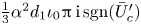 $\tfrac {1}{3}\alpha ^2d_1 \iota _0 {\rm \pi}\mathop {\rm i}\nolimits \mathop {\rm sgn}\nolimits (\bar U_c')$, as (3.17) indicates. This part is identical to
  $\tfrac {1}{3}\alpha ^2d_1 (a^+-a^-)$ according to (3.12), and thus cancel
  $-\tfrac {1}{3}\alpha ^2d_1d_1(a^+-a^-)$ in (3.19). As a result, the function
  $d_1(\tau,\bar {x})$, which can be determined by taking the analysis to
  $O(\epsilon ^{6/5})$ (cf. Wu & Tian Reference Wu and Tian2012), does not affect the key result (3.25). Equation (3.25) will lead to the required amplitude equation once the nonlinear jump
  $\mathscr {J}_d^{\mathcal {N}}$ is determined by the analysis in § 3.2. For that purpose, we note that the jump
  $(d_2^+ -d_2^-)$ is related to the jump of
  $\hat {u}_1$ across the critical level as follows:
 \begin{equation} \hat{u}_1(y=0^+)-\hat{u}_1(y=0^-)={-}\frac{3\bar{T}_c}{\alpha^2\bar{U}_c'}(d_2^+-d_2^-). \end{equation}
3.2. Critical-layer analysis
As was stated in § 2.2, the equations and solutions in the critical layer will be described in terms of the inner variable  $Y$ defined by (2.8). The disturbance characterising the CS in the critical layer could be expressed as
 \begin{equation} \tilde q(\zeta,\tau,\bar{x},Y,\theta)=\epsilon\sum_{j=j_0}^{\infty}\epsilon^{j/5}\tilde q_{j}(\zeta,\tau,\bar{x},Y,\theta) +\tilde q_L(\epsilon;\zeta,\tau,\bar{x},Y,\theta)\ln\epsilon,\end{equation}
where  $\tilde q$ also represents any of the velocity, pressure, temperature and density of the CS,
  $j_0$ indicates the magnitude of each quantity:
  $j_0=-2$ and
  $-1$ for
  $\tilde {T}$ and
  $\tilde {w}$ respectively, while
  $j_0=0$ for
  $\tilde {u}$,
  $\tilde {v}$ and
  $\tilde {p}$. The terms involving a logarithmic factor,
  $\tilde q_L$, are ignored owing to the fact that they match with the outer expansions automatically.
We further express  $\tilde {q}_j$ as Fourier series of
  $\zeta$ when it is necessary. For deriving the expected amplitude equation, it suffices to expand
  $\tilde q_j$ up to
  $\mathrm {e}^{2\mathop {\rm i}\nolimits \alpha \zeta }$ as
 \begin{equation} \tilde{q}_j=\sum_{n=0}^{2}\tilde{q}_{(\,j,n)}\mathrm{e}^{\mathop{\rm i}\nolimits n\alpha\zeta}+{\rm c.c.}+\cdots . \end{equation}
 It is recognised that  $\tilde {u}_1$,
  $\tilde {v}_3$,
  $\tilde {w}_0$,
  $\tilde {p}_3$ and
  $\tilde {T}_{-1}$ are driven by the primary nonlinear interactions and consist of the mean-flow distortion (
 $\tilde q_{(\,j,0)}+{\rm c.c.}$) and the first harmonic (
 $\tilde q_{(\,j,2)}\mathrm {e}^{2\mathop {\rm i}\nolimits \alpha \zeta }+{\rm c.c.}$). Similarly,
  $\tilde {u}_2$,
  $\tilde {v}_4$,
  $\tilde {w}_1$,
  $\tilde {p}_4$ and
  $\tilde {T}_0$ consist of the regenerated fundamental component (
 $\tilde q_{(\,j,1)}\mathrm {e}^{\mathop {\rm i}\nolimits \alpha \zeta }+{\rm c.c.}$), through which nonlinear effects enter the amplitude equation. Specifically, the axial velocity jump of the regenerated fundamental will be calculated and used to derive the modulation equation.
Substituting (3.27) into the CS equations, we obtain the equations within the critical layer. The inner solutions for  $\tilde {v}_0$,
  $\tilde {v}_1$,
  $\tilde {p}_0$,
  $\tilde {p}_1$ and
  $\tilde {p}_2$ are found to be simply the trivial continuations of the inviscid linear outer solutions, namely,
 \begin{gather} \tilde{v}_0 ={-}\mathop{\rm i}\nolimits {\hat{A}}/(\alpha\bar{U}_c') \mathrm{e}^{\mathop{\rm i}\nolimits\alpha\zeta}+{{\rm c.c.}}, \quad \tilde{v}_1=0;\end{gather}
 \begin{gather} \tilde{p}_0 ={\hat{A}}/(\alpha^2\bar{T}_c) \mathrm{e}^{\mathop{\rm i}\nolimits\alpha\zeta}+{{\rm c.c.}}, \quad \tilde{p}_1=0,\quad \tilde{p}_2=0,\end{gather}
where we have redefined the amplitude function as
 \begin{equation} {\hat{A}}=\alpha^2\bar{U}_c'A^{\dagger}. \end{equation}
The leading-order azimuthal velocity and temperature of the CS,  $\tilde {w}_{-1}$ and
  $\tilde {T}_{-2}$, satisfy
 \begin{equation} \left[{{\mathcal{L}}}_{c,1}^{\langle1\rangle}\tilde{T}_{{-}2} ,\ {{\mathcal{L}}}_{c,2}^{\langle1\rangle} \tilde{w}_{{-}1}\right] =\left[\mathop{\rm i}\nolimits\bar{T}_c'/(\alpha\bar{U}_c'), \ -\partial_\theta/(\alpha^2\breve{r}_c)\right]{\hat{A}} \mathrm{e}^{\mathop{\rm i}\nolimits\alpha\zeta}+{\rm c.c.}, \end{equation}
where the operator
 \begin{equation} {{\mathcal{L}}}_{c,j}^{\langle n\rangle}\equiv\frac{\partial}{\partial\tau}+\frac{\partial}{\partial\bar{x}} +\mathop{\rm i}\nolimits n\bar\eta+\chi\frac{\partial}{\partial\bar\eta}-\lambda_{jn}\frac{\partial^2}{\partial\bar\eta^2}, \end{equation}
in which the first two terms represent the non-equilibrium effect
 \begin{equation} \bar\eta=\alpha\left(\bar{U}_c'Y+\sigma\bar{U}_{1,c}\bar{x}\right), \end{equation}
denotes the shifted local radial variable in the critical layer and
 \begin{equation} \chi=\alpha\bar{U}_c'\sigma\left(\bar{U}_{1,c}/\bar{U}_c'+\bar{V}_c/c\right), \end{equation}
represents the non-parallelism (i.e. the axial variation and radial velocity) of the mean flow, which now manifests as the translating-critical-layer effect due to the dependence of the effective critical level on the variable  $\bar {x}$ (see (3.34));
  $\lambda _{jn}$ (
 $\,j=1,2$) characterise the complex viscosity and conductivity, introduced in the models for coherent Reynolds stresses, and have the expressions
 \begin{align} \left(\lambda_{1n}, \lambda_{2n}\right)=\alpha^2\bar{U}_c'^2\bar{T}_c\left(P\!r^{{-}1}\bar\lambda\mu_c +\widetilde{P\!r}_T^{{-}1}\tilde\lambda\tilde \mu_{t,c}\exp({\mathop{\rm i}\nolimits n\omega\hat\tau_2}),\quad \bar\lambda\mu_c+\tilde\lambda\tilde \mu_{t,c}\exp({\mathop{\rm i}\nolimits n\omega\hat\tau_1})\right). \end{align}
This is the first time that the effects of a translating critical layer and complex eddy viscosity have been included in weakly nonlinear dynamics. The solutions for  $\tilde {w}_{-1}$ and
  $\tilde {T}_{-2}$ are worked out as
 \begin{equation} \left[\tilde{T}_{{-}2}, \tilde{w}_{{-}1}\right]=\left\{\int_0^\infty \left[\frac{\mathop{\rm i}\nolimits\bar{T}_c'}{\alpha\bar{U}_c'} K_1^{(1)}, -\frac{1}{\alpha^2 \breve{r}_c} K_1^{(2)}\frac{\partial}{\partial\theta}\right]{\hat{A}}^{\;{\xi_1}} \exp({-\mathop{\rm i}\nolimits\bar\eta\xi_1})\,{\rm d}\xi_1\right\}\mathrm{e}^{\mathop{\rm i}\nolimits\alpha\zeta} +{\rm c.c.}, \end{equation}
where the integrand kernels
 \begin{equation} K_1^{(\,j)}(\xi)=\exp\left(-\lambda_{j1}\xi^3/3+\mathop{\rm i}\nolimits\chi \xi^2/2\right)\quad (\,j=1,2), \end{equation}
and the notation,
 \begin{equation} {\hat{A}}^{\;{\xi}}={\hat{A}}(\tau-\xi,\bar{x}-\xi,\theta), \end{equation}
is introduced to indicate the dependence on history. It is worth noting that the translating-critical-layer effect, the eddy viscosity and conductivity influence the kernel; this is a noteworthy difference from the laminar-flow case (cf. Wu Reference Wu1993).
The leading-order axial velocity of the CS,  $\tilde {u}_0$, is found to satisfy the equation
 \begin{align}
{{\mathcal{L}}}_{c,1}^{\langle1\rangle}\tilde{u}_0&={-}\bar{U}_c'\tilde{v}_2-\bar{T}_c\left(\frac{\partial\tilde{p}_2}{\partial\zeta}-\frac{\partial\tilde{p}_0}{c\partial\bar{x}}\right)-\left(\bar{U}_c''Y+\sigma\bar{U}_{1,c}'\bar{x}\right)\tilde{v}_0\nonumber\\
&\quad -\left(\bar{T}_c'Y+\sigma\bar{T}_{1,c}\bar{x}\right)\frac{\partial\tilde{p}_0}{\partial\zeta}
+\mu_c'\bar{T}_c\bar{U}_c'\frac{\partial\tilde{T}_{{-}2}}{\partial
Y} +\frac{\chi}{\alpha \bar{T}_c}\tilde{T}_{{-}2}.
\end{align}
\begin{align}
{{\mathcal{L}}}_{c,1}^{\langle1\rangle}\tilde{u}_0&={-}\bar{U}_c'\tilde{v}_2-\bar{T}_c\left(\frac{\partial\tilde{p}_2}{\partial\zeta}-\frac{\partial\tilde{p}_0}{c\partial\bar{x}}\right)-\left(\bar{U}_c''Y+\sigma\bar{U}_{1,c}'\bar{x}\right)\tilde{v}_0\nonumber\\
&\quad -\left(\bar{T}_c'Y+\sigma\bar{T}_{1,c}\bar{x}\right)\frac{\partial\tilde{p}_0}{\partial\zeta}
+\mu_c'\bar{T}_c\bar{U}_c'\frac{\partial\tilde{T}_{{-}2}}{\partial
Y} +\frac{\chi}{\alpha \bar{T}_c}\tilde{T}_{{-}2}.
\end{align}
The expansions of the continuity and energy equations at  $O(\epsilon )$ are combined to give
 \begin{equation} \frac{\partial \tilde{u}_0}{\partial\zeta}+\frac{\partial\tilde{v}_2}{\partial Y}+\frac{\tilde{v}_0}{r_c}+\frac{\partial\tilde{w}_{{-}1}}{\breve{r}_c\partial\theta}=\frac{\lambda_{11}}{\bar{T}_c}\frac{\partial^2\tilde{T}_{{-}2}}{\partial \bar\eta^2}.\end{equation}
With the aid of the scaled vorticity, introduced as
 \begin{equation} \tilde{Q}_j=\partial_Y \tilde{u}_j \quad (\,j=0,1,2),\end{equation}
we differentiate (3.40) with respect to  $Y$ to obtain
 \begin{equation} {{\mathcal{L}}}_{c,1}^{\langle1\rangle} \tilde{Q}_0={-}\tilde\lambda_{11}\frac{\bar{U}_c'}{\bar{T}_c}\frac{\partial^2\tilde{T}_{{-}2}}{\partial \bar\eta^2} +\chi\frac{\bar{U}_c'}{\bar{T}_c}\frac{\partial\tilde{T}_{{-}2}}{\partial \bar\eta} +\bar{U}_c'\left[\frac{1}{\breve{r}_c}\frac{\partial\tilde{w}_{{-}1}}{\partial\theta}+\left(\frac{1}{r_c}+\frac{\bar{T}_c'}{\bar{T}_c}-\frac{\bar{U}_c''}{\bar{U}_c'}\right)\tilde{v}_0\right],\end{equation}
where use has been made of (3.41), and we have put
 \begin{equation} \tilde\lambda_{1n}=\lambda_{1n}-\alpha^2\bar{U}_c'^2\bar{T}_c^2\bar\lambda\mu_c'. \end{equation}
Solving (3.43), we arrive at
 \begin{align}
\tilde{Q}_0&= \left\{\frac{\mathop{\rm
i}\nolimits\bar{T}_c'}{\alpha\bar{T}_c}\left(\frac{\tilde\lambda_{11}}{\lambda_{21}-\lambda_{11}}\right)\int_0^\infty
\left[\exp\left({(\lambda_{21}\!-\!\lambda_{11})\xi_1^3/3}\right)-1\right]
K_1^{(2)}(\xi_1){\hat{A}}^{\;{\xi_1}}\exp({-\mathop{\rm
i}\nolimits\bar\eta\xi_1})\,{\rm d}\xi_1\right.\nonumber\\
&\quad +\frac{\chi\bar{T}_c'}{\alpha\bar{T}_c}\int_0^\infty
K_\chi(\xi_1)K_1^{(2)}(\xi_1){\hat{A}}^{\;{\xi_1}}\exp({-\mathop{\rm
i}\nolimits\bar\eta\xi_1})\,{\rm d}\xi_1
-\frac{\bar{U}_c'}{\alpha^2\breve{r}_c^2}\int_0^\infty
\xi_1
K_1^{(2)}(\xi_1){\hat{A}}^{\;{\xi_1}}_{\theta\theta}\nonumber\\
&\left.\quad \times \exp({-\mathop{\rm
i}\nolimits\bar\eta\xi_1})\,{\rm d}\xi_1-\frac{\mathop{\rm
i}\nolimits\iota_0}{\alpha}\int_0^\infty \!
K_1^{(2)}(\xi_1){\hat{A}}^{\;{\xi_1}} \exp({-\mathop{\rm
i}\nolimits\bar\eta\xi_1})\,{\rm d}\xi_1\vphantom{\left\{\frac{\mathop{\rm
i}\nolimits\bar{T}_c'}{\alpha\bar{T}_c}\left(\frac{\tilde\lambda_{11}}{\lambda_{21}-\lambda_{11}}\right)\int_0^\infty
\left[\exp\left({(\lambda_{21}-\lambda_{11})\xi_1^3/3}\right)-1\right]
K_1^{(2)}(\xi_1){\hat{A}}^{\;{\xi_1}}\exp({-\mathop{\rm
i}\nolimits\bar\eta\xi_1})\,{\rm d}\xi_1\right.}\right\}
\exp({\mathop{\rm i}\nolimits\alpha\zeta})+{\rm c.c.},
\end{align}
\begin{align}
\tilde{Q}_0&= \left\{\frac{\mathop{\rm
i}\nolimits\bar{T}_c'}{\alpha\bar{T}_c}\left(\frac{\tilde\lambda_{11}}{\lambda_{21}-\lambda_{11}}\right)\int_0^\infty
\left[\exp\left({(\lambda_{21}\!-\!\lambda_{11})\xi_1^3/3}\right)-1\right]
K_1^{(2)}(\xi_1){\hat{A}}^{\;{\xi_1}}\exp({-\mathop{\rm
i}\nolimits\bar\eta\xi_1})\,{\rm d}\xi_1\right.\nonumber\\
&\quad +\frac{\chi\bar{T}_c'}{\alpha\bar{T}_c}\int_0^\infty
K_\chi(\xi_1)K_1^{(2)}(\xi_1){\hat{A}}^{\;{\xi_1}}\exp({-\mathop{\rm
i}\nolimits\bar\eta\xi_1})\,{\rm d}\xi_1
-\frac{\bar{U}_c'}{\alpha^2\breve{r}_c^2}\int_0^\infty
\xi_1
K_1^{(2)}(\xi_1){\hat{A}}^{\;{\xi_1}}_{\theta\theta}\nonumber\\
&\left.\quad \times \exp({-\mathop{\rm
i}\nolimits\bar\eta\xi_1})\,{\rm d}\xi_1-\frac{\mathop{\rm
i}\nolimits\iota_0}{\alpha}\int_0^\infty \!
K_1^{(2)}(\xi_1){\hat{A}}^{\;{\xi_1}} \exp({-\mathop{\rm
i}\nolimits\bar\eta\xi_1})\,{\rm d}\xi_1\vphantom{\left\{\frac{\mathop{\rm
i}\nolimits\bar{T}_c'}{\alpha\bar{T}_c}\left(\frac{\tilde\lambda_{11}}{\lambda_{21}-\lambda_{11}}\right)\int_0^\infty
\left[\exp\left({(\lambda_{21}-\lambda_{11})\xi_1^3/3}\right)-1\right]
K_1^{(2)}(\xi_1){\hat{A}}^{\;{\xi_1}}\exp({-\mathop{\rm
i}\nolimits\bar\eta\xi_1})\,{\rm d}\xi_1\right.}\right\}
\exp({\mathop{\rm i}\nolimits\alpha\zeta})+{\rm c.c.},
\end{align}where the second term is contributed by the translating-critical-layer effect, and
 \begin{equation} K_\chi(\xi_1)=\int_0^{\xi_1}\xi_2\exp({(\lambda_{21}-\lambda_{11})\xi_2^3/3})\,{\rm d}\xi_2;\end{equation}
the presence of this term is somewhat unexpected.
Consider the azimuthal momentum equation at  $O(\epsilon ^{7/5})$ and the energy equation at
  $O(\epsilon ^{6/5})$ for
  $\tilde {w}_{(0,0)}$ and
  $\tilde {T}_{(-1,0)}$
 \begin{equation} \left[{{\mathcal{L}}}_{c,1}^{\langle0\rangle} \tilde{T}_{({-}1,0)}, {{\mathcal{L}}}_{c,2}^{\langle0\rangle} \tilde{w}_{(0,0)}\right] ={-}\tilde{v}_{(0,1)}^*\partial_Y\left[\tilde{T}_{({-}2,1)}, \tilde{w}_{({-}1,1)}\right], \end{equation}
whose solutions are
 \begin{align}
\left[\tilde{T}_{({-}1,0)}, \tilde{w}_{(0,0)}\right] &=
\int_0^\infty\!\!\!\int_0^\infty
\xi_1{\hat{A}}^{\,*\,{\xi_2}}\left[-\frac{\mathop{\rm
i}\nolimits\bar{T}_c'}{\alpha\bar{U}_c'} K_2^{(1)},
\frac{1}{\alpha^2
\breve{r}_c}K_2^{(2)}\frac{\partial}{\partial\theta}\right]{\hat{A}}^{\;{\xi_1+\xi_2}} \nonumber\\
&\quad \times \exp({-\mathop{\rm i}\nolimits\bar\eta\xi_1}) \,{\rm
d}\xi_1\,{\rm d}\xi_2, \end{align}
\begin{align}
\left[\tilde{T}_{({-}1,0)}, \tilde{w}_{(0,0)}\right] &=
\int_0^\infty\!\!\!\int_0^\infty
\xi_1{\hat{A}}^{\,*\,{\xi_2}}\left[-\frac{\mathop{\rm
i}\nolimits\bar{T}_c'}{\alpha\bar{U}_c'} K_2^{(1)},
\frac{1}{\alpha^2
\breve{r}_c}K_2^{(2)}\frac{\partial}{\partial\theta}\right]{\hat{A}}^{\;{\xi_1+\xi_2}} \nonumber\\
&\quad \times \exp({-\mathop{\rm i}\nolimits\bar\eta\xi_1}) \,{\rm
d}\xi_1\,{\rm d}\xi_2, \end{align}where the integrand kernels
 \begin{equation} K_2^{(\,j)}(\xi_1,\xi_2)=\exp\left[-(\lambda_{j1}\xi_1^3+3\lambda_{j0}\xi_1^2\xi_2)/3+\mathop{\rm i}\nolimits\chi (\xi_1^2+2\xi_1\xi_2)/2\right]\quad (\,j=1,2). \end{equation}
 From the axial momentum equation at  $O(\epsilon ^{8/5})$, the equation for
  $\tilde {u}_{(1,0)}$ is derived as
 $$\begin{align}
{{\mathcal{L}}}_{c,1}^{\langle0\rangle}
\tilde{u}_{(1,0)}&={-}\tilde{v}_{(0,1)}^*\frac{\partial\tilde{u}_{(0,1)}}{\partial
Y}-\bar{U}_c'\tilde{v}_{(3,0)}
-(\bar{U}_c''Y+\sigma\bar{U}_{1,c}\bar{x})\tilde{v}_{(1,0)}-\tilde{T}_{({-}2,1)}\frac{\partial\tilde{p}_{(0,1)}^*}{\partial\zeta}\nonumber\\
&\quad +\,\mu_c'\bar{T}_c\bar{U}_c'\frac{\partial\tilde{T}_{({-}1,0)}}{\partial
Y}+\frac{\bar{U}_c'}{\bar{T}_c}\sigma\left(\bar{U}_{1,c}/\bar{U}_c'+\bar{V}_c/c\right)\tilde{T}_{({-}1,0)}.
\end{align}$$
$$\begin{align}
{{\mathcal{L}}}_{c,1}^{\langle0\rangle}
\tilde{u}_{(1,0)}&={-}\tilde{v}_{(0,1)}^*\frac{\partial\tilde{u}_{(0,1)}}{\partial
Y}-\bar{U}_c'\tilde{v}_{(3,0)}
-(\bar{U}_c''Y+\sigma\bar{U}_{1,c}\bar{x})\tilde{v}_{(1,0)}-\tilde{T}_{({-}2,1)}\frac{\partial\tilde{p}_{(0,1)}^*}{\partial\zeta}\nonumber\\
&\quad +\,\mu_c'\bar{T}_c\bar{U}_c'\frac{\partial\tilde{T}_{({-}1,0)}}{\partial
Y}+\frac{\bar{U}_c'}{\bar{T}_c}\sigma\left(\bar{U}_{1,c}/\bar{U}_c'+\bar{V}_c/c\right)\tilde{T}_{({-}1,0)}.
\end{align}$$
The expansion of the combined continuity and energy equations at  $O(\epsilon ^{6/5})$ for the mean-flow-distortion part gives
 \begin{equation} \frac{\partial\tilde{v}_{(3,0)}}{\partial Y}+\frac{\partial\tilde{w}_{(0,0)}}{\breve{r}_c\partial\theta}=\frac{\lambda_{10}}{\bar{T}_c}\frac{\partial^2\tilde{T}_{({-}1,0)}}{\partial\bar\eta^2},\end{equation}
with the aid of which we obtain from (3.50) the vorticity equation for  $\tilde {Q}_{(1,0)}\equiv \partial _Y\tilde {u}_{(1,0)}$
 \begin{align}
{{\mathcal{L}}}_{c,1}^{\langle0\rangle}\tilde{Q}_{(1,0)}&=\frac{\bar{U}_c'\partial\tilde{w}_{(0,0)}}{\breve{r}_c\partial\theta}-\tilde{v}_{(0,1)}^*\frac{\partial\tilde{Q}_{(0,1)}}{\partial
Y}
-\frac{\partial\tilde{p}_{(0,1)}^*}{\partial\zeta}\frac{\partial\tilde{T}_{({-}2,1)}}{\partial
Y} \nonumber\\
&\quad -\frac{\bar{U}_c'}{\bar{T}_c}\left[\tilde\lambda_{10}\frac{\partial^2}{\partial\bar\eta^2}
-\chi\frac{\partial}{\partial\bar\eta}\right]\tilde{T}_{({-}1,0)}.\end{align}
\begin{align}
{{\mathcal{L}}}_{c,1}^{\langle0\rangle}\tilde{Q}_{(1,0)}&=\frac{\bar{U}_c'\partial\tilde{w}_{(0,0)}}{\breve{r}_c\partial\theta}-\tilde{v}_{(0,1)}^*\frac{\partial\tilde{Q}_{(0,1)}}{\partial
Y}
-\frac{\partial\tilde{p}_{(0,1)}^*}{\partial\zeta}\frac{\partial\tilde{T}_{({-}2,1)}}{\partial
Y} \nonumber\\
&\quad -\frac{\bar{U}_c'}{\bar{T}_c}\left[\tilde\lambda_{10}\frac{\partial^2}{\partial\bar\eta^2}
-\chi\frac{\partial}{\partial\bar\eta}\right]\tilde{T}_{({-}1,0)}.\end{align}The solution is found as
 \begin{align} \tilde{Q}_{(1,0)}&=\frac{\bar{U}_c'}{\alpha^2\breve{r}_c^2}\int_0^\infty\!\!\!\int_0^\infty \xi_1^2 K_2^{(2)}(\xi_1,\xi_2){\hat{A}}^{\,*\,{\xi_2}}{\hat{A}}^{\;{\xi_1+\xi_2}}_{\theta\theta} \exp({-\mathop{\rm i}\nolimits\bar\eta\xi_1})\,{\rm d}\xi_1\,{\rm d}\xi_2\nonumber\\ &\quad +\frac{\bar{U}_c'}{\alpha^2\breve{r}_c^2}\int_0^\infty\!\!\!\int_0^\infty \xi_1\xi_2K_2^{(2)}(\xi_1,\xi_2)\left({\hat{A}}^{\,*\,{\xi_2}}{\hat{A}}^{\;{\xi_1+\xi_2}}_{\theta}\right)_{\theta} \exp({-\mathop{\rm i}\nolimits\bar\eta\xi_1})\,{\rm d}\xi_1\,{\rm d}\xi_2\nonumber\\ &\quad +\frac{\mathop{\rm i}\nolimits\iota_0}{\alpha}\int_0^\infty\!\!\!\int_0^\infty \xi_1 K_2^{(2)}(\xi_1,\xi_2){\hat{A}}^{\,*\,{\xi_2}}{\hat{A}}^{\;{\xi_1+\xi_2}} \exp({-\mathop{\rm i}\nolimits\bar\eta\xi_1})\,{\rm d}\xi_1\,{\rm d}\xi_2\nonumber\\ &\quad +\frac{\mathop{\rm i}\nolimits\bar{T}_c'}{\alpha\bar{T}_c}\int_0^\infty\!\!\!\int_0^\infty\xi_1 {\mathcal{C}}_{Q}(\xi_1,\xi_2)K_2^{(2)}(\xi_1,\xi_2){\hat{A}}^{\,*\,{\xi_2}}{\hat{A}}^{\;{\xi_1+\xi_2}} \exp({-\mathop{\rm i}\nolimits\bar\eta\xi_1})\,{\rm d}\xi_1\,{\rm d}\xi_2, \end{align}
where the last term is contributed by the temperature perturbation, and the kernel
 \begin{align}
{\mathcal{C}}_{Q}(\xi_1,\xi_2)&=\exp\left({(\lambda_{21}-\lambda_{11})\xi_1^3/3}\right)-{\tilde\lambda_{11}}({\lambda_{21}-\lambda_{11}})^{{-}1}
\left[\exp\left({(\lambda_{21}-\lambda_{11})\xi_1^3/3}\right)-1\right]\nonumber\\
&\quad +\mathop{\rm i}\nolimits\chi K_\chi(\xi_1)-\left({\tilde\lambda_{10}}-\mathop{\rm
i}\nolimits\chi\xi_1^{{-}1}\right)({\lambda_{20}-\lambda_{10}})^{{-}1} \nonumber\\
&\quad \times \exp\left({(\lambda_{21}-\lambda_{11})\xi_1^3/3}\right)
\left[\exp\left({(\lambda_{20}-\lambda_{10})\xi_1^2\xi_2}\right)-1\right].
\end{align}
\begin{align}
{\mathcal{C}}_{Q}(\xi_1,\xi_2)&=\exp\left({(\lambda_{21}-\lambda_{11})\xi_1^3/3}\right)-{\tilde\lambda_{11}}({\lambda_{21}-\lambda_{11}})^{{-}1}
\left[\exp\left({(\lambda_{21}-\lambda_{11})\xi_1^3/3}\right)-1\right]\nonumber\\
&\quad +\mathop{\rm i}\nolimits\chi K_\chi(\xi_1)-\left({\tilde\lambda_{10}}-\mathop{\rm
i}\nolimits\chi\xi_1^{{-}1}\right)({\lambda_{20}-\lambda_{10}})^{{-}1} \nonumber\\
&\quad \times \exp\left({(\lambda_{21}-\lambda_{11})\xi_1^3/3}\right)
\left[\exp\left({(\lambda_{20}-\lambda_{10})\xi_1^2\xi_2}\right)-1\right].
\end{align} At the next order,  $\tilde {u}_2$, or the corresponding vorticity
  $\tilde {Q}_2\equiv \partial _Y\tilde {u}_2$, is coupled with
  $\tilde {v}_4$,
  $\tilde {w}_1$,
  $\tilde {p}_4$ and
  $\tilde {T}_0$. In order to work out the jump of
  $\tilde {u}_{(2,1)}$ across the critical layer, we split the quantities at this order, any of which is denoted by
  $\tilde {q}_{(\,j,1)}$, into three parts
 \begin{equation} \tilde{q}_{(\,j,1)}=\tilde{q}_{(\,j,1)}^{\mathcal{N}}+\tilde{q}_{(\,j,1)}^{{O}}+\tilde{q}_{(\,j,1)}^{\mathcal{L}}, \end{equation}
where  $q_{(\,j,1)}^{\mathcal {L}}$ represents the linear part, while
  $\tilde {q}_{(\,j,1)}^{\mathcal {N}}$ and
  $\tilde {q}_{(\,j,1)}^{{O}}$ denote the nonlinear parts which do and do not contribute to the jump respectively. It turns out that the nonlinear terms
  $\tilde {v}_{(0,1)}\partial _Y \tilde {q}_{(\,j-1,0)}$ and
  $\tilde {v}_{(0,1)}^*\partial _Y \tilde {q}_{(\,j-1,2)}$ produce no contribution to the jump and hence are included in
  $\tilde {q}_{(\,j,1)}^{{O}}$. The jump of
  $(d_2^+-d_2^-)$ can be found after integrating
  $\tilde {Q}_{(2,1)}$ with respect to
  $Y$ from
  $-\infty$ to
  $\infty$, and would consist of the linear and nonlinear parts,
  ${\mathscr J}_d^{\mathcal {L}}$ and
  ${\mathscr J}_d^{\mathcal {N}}$. The former confirms the
  $-{\rm \pi}$ phase jump of the logarithm in the outer expansion
  $\hat {u}_2$. The latter is contributed by
  $\tilde {Q}_{(2,1)}^{\mathcal {N}}\equiv \partial _Y\tilde {u}_{(2,1)}^{\mathcal {N}}$, which satisfies the equation
 \begin{align}
{{\mathcal{L}}}_{c,1}^{\langle1\rangle}
\tilde{Q}_{(2,1)}^{\mathcal{N}}&=\bar{U}_c'\frac{\partial\tilde{w}_{(1,1)}^{\mathcal{N}}}{\breve{r}_c\partial\theta}
-\tilde{v}_{(0,1)}\frac{\partial
\tilde{Q}_{(1,0)}^*}{\partial Y}
-\frac{\partial\tilde{p}_{(0,1)}}{\partial\zeta}\frac{\partial\tilde{T}_{({-}1,0)}^*}{\partial
Y} \nonumber\\
&\quad -\tilde\lambda_{11}\frac{\bar{U}_c'}{\bar{T}_c}\frac{\partial^2\tilde{T}_{(0,1)}^{\mathcal{N}}}{\partial\bar\eta^2}
+\chi\frac{\bar{U}_c'}{\bar{T}_c}\frac{\partial\tilde{T}_{(0,1)}^{\mathcal{N}}}{\partial\bar\eta};\end{align}
\begin{align}
{{\mathcal{L}}}_{c,1}^{\langle1\rangle}
\tilde{Q}_{(2,1)}^{\mathcal{N}}&=\bar{U}_c'\frac{\partial\tilde{w}_{(1,1)}^{\mathcal{N}}}{\breve{r}_c\partial\theta}
-\tilde{v}_{(0,1)}\frac{\partial
\tilde{Q}_{(1,0)}^*}{\partial Y}
-\frac{\partial\tilde{p}_{(0,1)}}{\partial\zeta}\frac{\partial\tilde{T}_{({-}1,0)}^*}{\partial
Y} \nonumber\\
&\quad -\tilde\lambda_{11}\frac{\bar{U}_c'}{\bar{T}_c}\frac{\partial^2\tilde{T}_{(0,1)}^{\mathcal{N}}}{\partial\bar\eta^2}
+\chi\frac{\bar{U}_c'}{\bar{T}_c}\frac{\partial\tilde{T}_{(0,1)}^{\mathcal{N}}}{\partial\bar\eta};\end{align}the derivation is given in Zhang (Reference Zhang2022).
To find  $\tilde {w}_{(1,1)}^{\mathcal {N}}$ and
  $\tilde {T}_{(0,1)}^{\mathcal {N}}$ on the right-hand side of (3.56), we consider the azimuthal momentum equation at
  $O(\epsilon ^{8/5})$ and the energy equation at
  $O(\epsilon ^{7/5})$, which read
 \begin{equation} \left[{{\mathcal{L}}}_{c,1}^{\langle1\rangle} \tilde{T}_{(0,1)}^{\mathcal{N}}, {{\mathcal{L}}}_{c,2}^{\langle1\rangle} \tilde{w}_{(1,1)}^{\mathcal{N}}\right] ={-}\tilde{v}_{(0,1)}{\partial_Y}\left[\tilde{T}_{({-}1,0)}^*, \tilde{w}_{(0,0)}^*\right]. \end{equation}
The solutions are found as
 $$\begin{align} \left[\tilde{T}_{(0,1)}^{\mathcal{N}}, \tilde{w}_{(1,1)}^{\mathcal{N}}\right]&={-}\int_0^\infty\!\!\!\int_0^\infty\!\!\!\int_0^\infty\xi_3^2{\hat{A}}^{\;{\xi_1}}{\hat{A}}^{\;{\xi_1+\xi_2}}\left[\frac{\mathop{\rm i}\nolimits\bar{T}_c'}{\alpha\bar{U}_c'}K_3^{(1)}, \frac{1}{\alpha^2\breve{r}_c}K_3^{(2)}\frac{\partial}{\partial\theta}\right]{\hat{A}}^{\,*\,{\xi_1+\xi_2+\xi_3}}\nonumber\\ &\quad \times\exp\left({-\mathop{\rm i}\nolimits\bar\eta(\xi_1-\xi_3)}\right)\,{\rm d}\xi_1\,{\rm d}\xi_2\,{\rm d}\xi_3, \end{align}$$
where the integrand kernels
 $$\begin{gather} K_3^{(\,j)}(\xi_1,\xi_2,\xi_3)=\exp\left[-\lambda_{j1}\left(\xi_1^3-3\xi_1^2\xi_3+3\xi_1\xi_3^2\right)/3-\lambda_{j1}^*\xi_3^3/3-\lambda_{j0}^*\xi_2\xi_3^2\right.\nonumber\\ \left.+\mathop{\rm i}\nolimits\chi\left(\xi_1^2-2\xi_1\xi_3-\xi_3^2-2\xi_2\xi_3\right)/2\right] \quad (\,j=1,2). \end{gather}$$
 Inserting (3.58) along with (3.29)–(3.30), (3.37b) and (3.53) into (3.56), and integrating  $\tilde {Q}_{(0,1)}^{\mathcal {N}}$ with respect to
  $Y$ from
  $-\infty$ to
  $\infty$, we arrive at the nonlinear part of
  $d_2^\pm$
 \begin{equation} {\mathscr J}_d^{\mathcal{N}}={\mathscr N}_{\varTheta}+ {\mathscr N}_{U}+{\mathscr N}_{T}, \end{equation}
where
 \begin{align} {\mathscr N}_{\varTheta}({\hat{A}};\tau,\bar{x},\theta) =\frac{2{\rm \pi}\bar{U}_c'^2}{3\alpha|\bar{U}_c'|\bar{T}_c \breve{r}_c^2}\int_0^\infty\!\!\!\int_0^\infty \hat{\mathcal{A}}_{\varTheta}({\hat{A}};\,\xi_1,\xi_2)\,K_\varTheta(\xi_1,\xi_2)\,{\rm d}\xi_1\,{\rm d}\xi_2, \end{align}
 \begin{align} {\mathscr N}_{U}({\hat{A}};\tau,\bar{x},\theta) ={-}\frac{2{\rm \pi}\mathop{\rm i}\nolimits\bar{U}_c'\iota_0}{3|\bar{U}_c'|\bar{T}_c}\int_0^\infty\!\!\!\int_0^\infty \hat{\mathcal{A}}_{N}({\hat{A}};\,\xi_1,\xi_2)\,K_U(\xi_1,\xi_2)\,{\rm d}\xi_1\,{\rm d}\xi_2, \end{align}
 \begin{align} {\mathscr N}_{T}({\hat{A}};\tau,\bar{x},\theta)={-}\frac{2{\rm \pi}\mathop{\rm i}\nolimits\bar{U}_c'\bar{T}_c'}{3|\bar{U}_c'|\bar{T}_c^2}\int_0^\infty\!\!\!\int_0^\infty \hat{\mathcal{A}}_{N}({\hat{A}};\,\xi_1,\xi_2)\,K_T(\xi_1,\xi_2)\,{\rm d}\xi_1\,{\rm d}\xi_2; \end{align}
here, we have introduced notations
 \begin{gather} \hat{\mathcal{A}}_{\varTheta}({\hat{A}};\,\xi_1,\xi_2)= \xi_1\left[{\hat{A}}^{\;{\xi_1}}{\hat{A}}^{\;{\xi_1+\xi_2}}{\hat{A}}^{\,*\,{2\xi_1+\xi_2}}_{\theta}\right]_{\theta} +\xi_1{\hat{A}}^{\;{\xi_1}}{\hat{A}}^{\;{\xi_1+\xi_2}}{\hat{A}}^{\,*\,{2\xi_1+\xi_2}}_{\theta\theta}\nonumber\\ \quad\ +\,\xi_2{\hat{A}}^{\;{\xi_1}}\left[{\hat{A}}^{\;{\xi_1+\xi_2}}{\hat{A}}^{\,*\,{2\xi_1+\xi_2}}_{\theta}\right]_{\theta}, \end{gather}
 \begin{gather} \hat{\mathcal{A}}_{N}({\hat{A}};\,\xi_1,\xi_2)\,={\hat{A}}^{\;{\xi_1}}{\hat{A}}^{\;{\xi_1+\xi_2}}{\hat{A}}^{\,*\,{2\xi_1+\xi_2}}, \end{gather}
the kernels in which have the expressions
 \begin{gather} K_\varTheta(\xi_1,\xi_2)=K_U(\xi_1,\xi_2)=\xi_1^2 K_J^{(2)}(\xi_1,\xi_2),\end{gather}
 \begin{gather} K_T(\xi_1,\xi_2)=\xi_1^2\left[{\mathcal{C}}_T(\xi_1)K_J^{(1)}(\xi_1,\xi_2) +{\mathcal{C}}_Q^*(\xi_1,\xi_2)K_J^{(2)}(\xi_1,\xi_2)\right],\end{gather}
with
 \begin{align} K_J^{(\,j)}(\xi_1,\xi_2)&=\exp\left[-\left(\lambda_{j1}+\lambda_{j1}^*\right)\xi_1^3/3 -\lambda_{j0}^*\xi_1^2\xi_2-\mathop{\rm i}\nolimits\chi(\xi_1^2+\xi_1\xi_2)\right]\quad (\,j=1,2), \end{align}
 $$\begin{align}
{\mathcal{C}}_T(\xi_1)&=\exp\left({-(\lambda_{21}-\lambda_{11})\xi_1^3/3}\right)+{\tilde\lambda_{11}}({\lambda_{21}
-\lambda_{11}})^{{-}1} \nonumber\\
&\quad \times \left[\exp\left({-(\lambda_{21}-\lambda_{11})\xi_1^3/3}\right)-1\right]-\mathop{\rm i}\nolimits\chi K_\chi(-\xi_1).
\end{align}$$
$$\begin{align}
{\mathcal{C}}_T(\xi_1)&=\exp\left({-(\lambda_{21}-\lambda_{11})\xi_1^3/3}\right)+{\tilde\lambda_{11}}({\lambda_{21}
-\lambda_{11}})^{{-}1} \nonumber\\
&\quad \times \left[\exp\left({-(\lambda_{21}-\lambda_{11})\xi_1^3/3}\right)-1\right]-\mathop{\rm i}\nolimits\chi K_\chi(-\xi_1).
\end{align}$$3.3. Amplitude equation and its upstream condition
Inserting (3.60) into (3.25), we arrive at the expected amplitude equation
 \begin{equation} \frac{\partial{\hat{A}}}{\partial\bar{x}}+\frac{1}{c_g}\frac{\partial{\hat{A}}}{\partial\tau} -\frac{1}{c_h}\frac{\partial^2{\hat{A}}}{\breve{r}_c^2\partial\theta^2}=\sigma_s\bar{x}{\hat{A}} +\sigma_N \left({\mathscr N}_{\varTheta}+ {\mathscr N}_{U}+{\mathscr N}_{T}\right), \end{equation}
where
 \begin{equation} \left. \begin{gathered} c_g=\varsigma_w/\left[{2\mathop{\rm i}\nolimits}J_{r2}/{\alpha}-{{\rm \pi}\alpha}\left(\,j_R-2\iota_0^2\right)/\left({\left|\bar{U}_c'\right|\bar{T}_c}\right)\right],\quad c_h=\varsigma_w/{J_h},\\ \sigma_s=\sigma\left\{J_{r0}+{{\rm \pi}\mathop{\rm i}\nolimits\alpha^2\left[\bar{U}_{1,c} \left(\,j_R-2\iota_0^2\right)-\bar{U}_c'j_{1R}\right]}/\left({\left|\bar{U}_c'\right|\bar{T}_c}\right)\right\}/\varsigma_w,\\ \sigma_N={-}{3\alpha^2}/{\varsigma_w},\quad \varsigma_w={2\mathop{\rm i}\nolimits}\left(J_{r2}-{J_{r1}}/{c}\right)/{\alpha}-{{\rm \pi}\alpha} \left(\,j_R-2\iota_0^2\right)/\left({\left|\bar{U}_c'\right|\bar{T}_c}\right). \end{gathered} \right\} \end{equation}
Here,  $c_g$ is the complex group velocity. The integro-partial-differential equation (3.66) describes the simultaneous axial evolution and temporal–azimuthal modulation under the combined effects of viscosity, nonlinearity and non-parallelism.
In the general case where the CS is superposition of the ring and helical modes, the amplitude function  ${\hat {A}}$ can be decomposed as
 \begin{equation} {\hat{A}}(\tau,\bar{x},\theta)=\sum_{m={-}\infty}^{\infty}A^{[m]}(\tau,\bar{x})\mathrm{e}^{\mathop{\rm i}\nolimits m \theta}, \end{equation}
from which follows the relation  $A^{[m]*}=A^{*[-m]}$. We introduce an overall amplitude to characterise the multiple ring-/helical-mode CS,
 \begin{equation} A_{\mathcal{H}}(\tau,\bar{x})=\sqrt{\sum_{m={-}\infty}^{\infty}\left|A^{[m]}(\tau,\bar{x})\right|^2}.\end{equation}
It should be noted that the Fourier component of nonlinear products should be understood as a triple discrete convolution or a triple Cauchy product.
To determine the self-consistent upstream condition, we note that the nonlinear term  ${\mathscr J}_d^{\mathcal {N}}$ is negligible since the amplitudes of the seeded modes upstream are small. The linear limit of (3.66) is solved to give the upstream condition
 \begin{equation} A^{[m]} \rightarrow A^{[m]}_0\exp\left[\sigma_s\bar{x}^2/2+\kappa^{[m]}\bar{x}-\mathop{\rm i}\nolimits S_0\tau\right] \quad \text{as} \bar{x}\rightarrow-\infty, \end{equation}
in which  $A^{[m]}_0$ is the complex initial amplitude of the seeded mode with azimuthal wavenumber
  $m$, and it has modulus
  $a_0^{[m]}$ and initial phase
  $\phi _0^{[m]}$, i.e.
 \begin{equation} A^{[m]}_0=a^{[m]}_0\mathrm{e}^{\mathop{\rm i}\nolimits \phi_0^{[m]}}, \end{equation}
where  $S_0$ is the deviation of the frequency from that of the neutral mode, i.e. the frequency of the CS is
  $\omega =\alpha c+\epsilon ^{2/5}S_0$, and
 \begin{equation} \kappa^{[m]}=\mathop{\rm i}\nolimits S_0/c_g-m^2/c_h, \end{equation}
is the correction to the complex axial wavenumber. The real part of  $\kappa ^{[m]}$,
  $\Re (\kappa ^{[m]})$, denotes the (scaled) linear growth rate of each ring/helical mode.
4. Theoretical considerations of the evolution equation
4.1. Singularity and nonlinearity
Nonlinear effects are associated with four types of singularities in the inviscid linear solution of nearly neutral modes constituting the CS (Wu Reference Wu2019): (a) the simple-pole singularity in the velocity due to three-dimensionality; (b) the simple-pole singularity in the temperature; (c) the primary logarithmic singularity for a non-inflectional point mode (Zhang Reference Zhang2022); (d) the secondary logarithmic singularity due to the non-equilibrium effect. When regularised in the critical layer, each of the singularities represents a large disturbance and thus contributes a nonlinear term in the evolution equation.
As was shown in [II], the evolution of pure ring-mode CS is governed by a strongly nonlinear theory because the nonlinearities associated with compressibility and non-equilibrium are made comparable by taking the mean-temperature gradient at the critical level to be small. The evolution of multiple ring and helical modes takes a weakly nonlinear form because the nonlinear interactions among ring/helical modes take place at a lower amplitude than that between a ring mode and its harmonics does.
In the nonlinear amplitude equation (3.66), the left-hand side represents the axial evolution and the temporal–azimuthal modulation, while the right-hand side consists of the effects of non-parallelism and nonlinearity. The latter is composed of three parts. The nonlinear term  ${\mathscr N}_{\varTheta }$ is associated with three-dimensionality, measured by
  $\breve {r}_c^{-2}$,
  ${\mathscr N}_{U}$ is with non-inflectional nature of the critical layer (
 $\iota _0$) (Zhang Reference Zhang2022), which vanishes for CS of subsonic modes, while
  ${\mathscr N}_{T}$ is contributed by compressibility, measured by
  $\bar {T}_c'$. The amplitude equation (3.66) reduces to that for the incompressible regime by setting
  $\bar {T}_c'=0$. Furthermore, with
  $\breve {r}_c\theta$ being interpreted as
  $Z=\epsilon ^{2/5}z$, the scaled slow spanwise variable, the nonlinear terms in the amplitude equation (3.66) resemble those describing the nonlinear evolution of the near-planar waves on planar shear layers (Wu Reference Wu1993), but the kernels are modified by non-parallelism and complex eddy viscosity.
4.2. Modal composition and nonlinearity
When only one ring or helical mode is seeded upstream, the nonlinear interaction does not generate additional unseeded modes so that  ${\hat {A}}$ takes the form
 \begin{equation} {\hat{A}}(\tau,\bar{x},\theta)= A_S(\tau,\bar{x})\mathrm{e}^{\mathop{\rm i}\nolimits m\theta}, \end{equation}
and it follows that the nonlinear terms  $\hat {\mathcal {A}}_{\varTheta }$ and
  $\hat {\mathcal {A}}_{N}$ become
 \begin{equation} \hat{\mathcal{A}}_{\varTheta}\equiv 0,\quad \hat{\mathcal{A}}_{N}=A_S^{\;{\xi_1}}A_S^{\;{\xi_1+\xi_2}}A_S^{\,*\,{2\xi_1+\xi_2}} \mathrm{e}^{\mathop{\rm i}\nolimits m\theta}. \end{equation}
As a result, the factor  $\mathrm {e}^{\mathop {\rm i}\nolimits m\theta }$ drops out of the amplitude equation, which simplifies to the one for
  $A_S(\tau,\bar {x})$. The three-dimensional nonlinearity does not influence the dynamics of a single helical mode, the nonlinear effects on which are associated with the compressibility and logarithmic singularities, measured by
  $\bar {T}_c'$ and
  $\iota _0$ respectively. This is consistent with the Squire transformation, which converts a three-dimensional wave into an equivalent two-dimensional counterpart; see Goldstein & Leib (Reference Goldstein and Leib1989) and Leib (Reference Leib1991). For a subsonic mixing layer and jet,
  $\bar {T}_c'$, which controls the nonlinearity due to compressibility, turned out to be numerically small for a range of
  $M\!a$, as was pointed out by Sparks & Wu (Reference Sparks and Wu2008), [I] and [II]. This led them to take
  $\bar {T}_c'$ as a small parameter such that the nonlinearity due to compressibility is comparable to that associated with the secondary logarithmic singularity of the axial velocity of the mode. A strongly nonlinear critical-layer theory emerges. Similarly, when only one ring or helical mode is seeded upstream, the present weakly nonlinear theory is unlikely to be accurate or appropriate (see e.g. figure 2a), and a strongly nonlinear theory is required instead.

Figure 2. Amplitude evolution with different modes seeded upstream. (a) A single  $m=1$ mode (dashed line), a pair of
  $m=\pm 1$ modes with identical initial amplitude (the solid line without circles) and a pair of
  $m=\pm 1$ modes of different initial amplitudes with ratio
  $a_0^{[-1]}/a_0^{[1]}=0.5$ (the solid lines with circles); (b) development of nonlinearly generated modes: solid lines for
  $|m|=1$, dashed lines for
  $|m|=3$, dash–dotted lines for
  $|m|=5$, dotted lines for
  $|m|=7$: lines without circles represent the helical modes with identical initial amplitude (
 $a_0^{[-1]}/a_0^{[1]}=1$) and lines with filled/empty circles represent the helical modes with
  $m\gtrless 0$ and initial amplitude ratio
  $a_0^{[-1]}/a_0^{[1]}=0.5$.
When two modes, whose azimuthal wavenumbers are  $m_1$ and
  $m_2$ with the difference
  $m_\nu =|m_1-m_2|\neq 0$, are seeded upstream, the self-interaction of each mode generates an axisymmetric mean-flow distortion, whereas the mutual interactions of the two generate streaks with azimuthal wavenumbers
  $\pm m_\nu$. The modes
  $\pm m_\nu$ interact at the cubic level with the fundamental to excite modes with azimuthal wavenumbers
  $m_1\pm m_\nu$, or
  $m_2\pm m_\nu$. Further interactions at higher orders with the seeded and newly excited modes generate more azimuthal components
  $m_1\pm n m_\nu$ or
  $m_2\pm n m_\nu$ (
 $n \in \mathbb {Z}$) so that the azimuthal-wavenumber spectrum is expected to broaden.
4.3. Laminar case
The amplitude equation for CS on a turbulent jet, (3.66), is applicable to the wavepackets of instability modes on a laminar shear flow as a special case. For a laminar flow, the coherent Reynolds stresses disappear. The radial velocity of the base flow is of  $O({\textit {Re}}^{-1})$, smaller than that in the turbulent case, and the axial variation of a laminar base-flow profile is slower, occurring on the slow axial variable
  $\tilde {x}_L={\textit {Re}}^{-1}x$ instead of
  $\tilde {x}=R_T^{-1}x$ for a turbulent mean flow. We can thus drop the term representing the non-parallelism,
  $\sigma _s \bar {x} {\hat {A}}$, from (3.66), and in the nonlinear terms set
  $\sigma =0$ (so that
  $\chi =0$) and
  $\tilde \lambda =0$. Correspondingly, the kernel in the nonlinear term due to compressibility reduces to that in Leib (Reference Leib1991), in which the viscosity law,
  $\mu =\bar {T}^n$, was used.
Despite the slow variation of a laminar base flow, the non-parallelism may have an appreciable effect on the evolution. We may derive a composite theory to include effects of both non-equilibrium and non-parallelism as was done in Wu & Huerre (Reference Wu and Huerre2009).
4.4. Weak compressibility and weaker three-dimensionality limits
When three-dimensionality is weaker than assumed, i.e.  $\breve {r}_c^{-2}\ll 1$, but the flow is fully compressible with
  $\bar {T}_c'=O(1)$, the amplitude equation (3.66) reduces to
 \begin{equation} \frac{\partial{\hat{A}}}{\partial\bar{x}}+\frac{1}{c_g}\frac{\partial{\hat{A}}}{\partial\tau}=\sigma_s\bar{x}{\hat{A}} +\sigma_N{\mathscr N}_{T}({\hat{A}};\tau,\bar{x},\theta),\end{equation}
in which the nonlinearity is contributed only by compressibility, and the dependence on  $\theta$ is entirely parametric. On the other hand, when the flow is weakly compressible with
  $\bar {T}_c'\ll 1$ but
  $\breve {r}_c^{-2}=O(1)$, we may drop
  ${\mathscr N}_{T}$ to obtain
 \begin{equation} \frac{\partial{\hat{A}}}{\partial\bar{x}}+\frac{1}{c_g}\frac{\partial{\hat{A}}}{\partial\tau} -\frac{1}{c_h}\frac{\partial^2{\hat{A}}}{\breve{r}_c^2\partial\theta^2} =\sigma_N{\mathscr N}_{\varTheta}({\hat{A}};\tau,\bar{x},\theta) +\sigma\!_N{\mathscr N}_{U}({\hat{A}};\tau,\bar{x},\theta). \end{equation}
 However, neither (4.3) nor (4.4) represents a distinguished regime. A distinguished regime arises when both compressibility and three-dimensionality are weaker than assumed. We discuss this for a regular critical layer ( $\iota _0=0$), and introduce
 \begin{equation} \breve{r}_c^{{-}1}=l_{\dot\beta} \dot{\breve{r}}_c^{{-}1},\quad \bar{T}_c'=l_{\dot\beta}^2\dot{\bar{T}}_c', \end{equation}
with  $l_{\dot \beta }\ll 1$ and
  $\dot{\breve {r}}_c^{-1}\sim \dot {\bar {T}}_c'=O(1)$ to retain the two types of nonlinearity. Inserting them into (3.66) and rescaling
  $A=l_{\dot \beta }^{-1}\dot A$, we obtain its limiting form
 \begin{equation} \frac{\partial\dot A}{\partial\bar{x}}+\frac{1}{c_g}\frac{\partial\dot A}{\partial\tau} =\sigma_N{\mathscr N}_{\varTheta}(\dot{\breve{r}}_c^{{-}1},\dot A;\tau,\bar{x},\theta) +\sigma_N{\mathscr N}_{T}(\dot{\bar{T}}_c',\dot A;\tau,\bar{x},\theta). \end{equation}
In this situation, the linear growth rate remains of  $O(l_\gamma )=O(\epsilon ^{2/5})$, while the unscaled amplitude is increased to the order of
  $\dot \epsilon =\epsilon l_{\dot \beta }^{-1}$. When the unscaled amplitude
  $\dot \epsilon$ is increased to
  $O(l_\gamma ^2)$, namely,
  $l_{\dot \beta }=O(\epsilon ^{1/5})$, the limiting form (4.6) would break down because a strongly nonlinear critical layer arises. The present theory, together with its limiting form, remains valid for
  $\epsilon ^{-1/5}\leqslant r_c \ll \epsilon ^{-2/5}$. When
  $r_c^{-1}=O(\epsilon ^{2/5})=O(\dot {\epsilon }^{1/2})$, which is realised in a ‘very-near-nozzle’ region, a strongly nonlinear theory is required to describe the interactions of an arbitrary number of coexisting ring and helical modes. This case will be reported in a separate paper.
Other limiting cases include the ‘very non-parallel’ and ‘very viscous’ regimes, in each of which the amplitude equation (3.66) simplifies as is discussed in Zhang (Reference Zhang2022).
4.5. Terminal forms
Mathematical considerations, aided by numerical results, suggest three possible terminal forms of solutions, which the disturbance may attain as  $\bar {x}\rightarrow \infty$ or at a finite axial distance
  $\bar {x}_s$. Their occurrence depends on the size of the initial amplitude.
When the initial amplitude is small enough, the entire evolution remains practically linear, taking the form (3.70). For moderate initial amplitudes, the most common evolution scenario is that following the linear stage the modes in the wavepacket interact with each other, causing oscillatory saturation and eventual attenuation. Since the non-parallelism and viscous effects cause ‘memory decay’, as indicated by the kernels, nonlinear terms diminish and the modes become independent in the final relaxation stage with the amplitude of each mode resuming the form (3.70).
The second terminal form is that the amplitudes of the modes in the CS blow up at a finite downstream distance  $\bar {x}_s$. As
  $\bar {x}\rightarrow \bar {x}_s$, the amplitude of each mode has the structure
 \begin{equation} A^{[m]} \rightarrow a^{[m]}_T/(\bar{x}_s-\bar{x})^{5/2+\mathop{\rm i}\nolimits\sigma_T}, \end{equation}
where  $a^{[m]}_T$ and
  $\sigma _T$ are complex and real, respectively. The present form of singularity is a generalisation of that for a single mode (Goldstein & Leib Reference Goldstein and Leib1989; Leib Reference Leib1991) to the multiple-mode case. Substitution of (4.7) into the governing equations of
  $A^{[m]}$ leads to a system of coupled nonlinear algebraic equations for
  $a_T^{[m]}$ and
  $\sigma _T$; see Zhang (Reference Zhang2022) for the detail. The value of
  $\bar {x}_s$ depends on the composition and size of the seeded modes, and has to be determined numerically. In the vicinity of
  $\bar {x}_s$, the present theory breaks down, and the disturbance is likely to enter a fully nonlinear stage, where the amplitude would evolve on the same short length scale as the wavelength, and the Euler or N–S equations have to be called upon (cf. Goldstein & Leib Reference Goldstein and Leib1989). A full resolution of the singularity is beyond scope of the present study.
Finally, we consider the focusing singularity of the form in Wu (Reference Wu1993), namely,
 \begin{equation} {\hat{A}}= F(\hat\theta)/(\bar{x}_s-\bar{x})^{{5/2}+\mathop{\rm i}\nolimits\sigma_T},\quad \hat\theta=(\theta-\theta_s)/(\bar{x}_s-\bar{x})^{1/2}, \end{equation}
where  $\theta _s$ is azimuthal angle at which the CS concentrates. Inserting (4.8a,b) into (3.66), we obtain the integro–differential equation for
  $F(\hat \theta )$, which is given in Zhang (Reference Zhang2022). This type of singularity is associated with both the two- and three-dimensional nonlinear terms, which are of the same order. Numerical solutions indicate a trend of azimuthal focusing, but there is no firm evidence of the eventual formation of the singularity.
5. Numerical solutions of the amplitude evolution equation
The theory is applied to a compressible turbulent jet, in which the mean flow is formed between the exhaust flow,  $(U_{I}^*,T^*_{I})$, and a co-flow,
  $(U_{O}^*,T^*_{O})$ (
 $U_{O}^*< U_{I}^*$ appropriately assumed). The axial mean-flow velocity is chosen to have a self-similar profile
 \begin{equation} \bar{U}\left[\eta^{\dagger}\left(y,\tilde{x}\right)\right]=\bar{U}_{R}+f(\eta^{\dagger}),\end{equation}
with  $f(\eta ^{\dagger} )=-(1+q_c\mathop {\rm sech}\nolimits ^2\!\eta ^{\dagger} )\tanh (\eta ^{\dagger} )$
 \begin{equation} \bar{U}_{R}=\frac{U_{\text{I}}^*+U_{\text{O}}^*}{U_{\text{I}}^*-U_{\text{O}}^*}=\frac{1+\beta_U}{1-\beta_U},\quad \eta^{\dagger} (\tilde{x},r)=\eta_{c}^{\dagger}+\frac{r-r_T(\tilde{x})}{\delta_T(\tilde{x})}\quad (r > 0), \end{equation}
where  $\beta _U=U_{O}^*/U_{I}^*$;
  $\eta ^{\dagger}$ is the self-similar variable with
  $\eta _{c}^{\dagger}$ being introduced to ensure that the critical level
  $r=r_c$ at the neutral position
  $\tilde {x}=\tilde {x}_N$ is located at
  $r=r_T(\tilde {x}_N)$;
  $r_T$ and
  $\delta _T$ are functions of
  $\tilde {x}$, standing for the equivalent central position and the thickness of the shear layer, respectively. The phase speed of the neutral mode,
  $c$, is given by
 \begin{equation} c=\bar{U}_c=\bar{U}_{R}+f\left(\eta_{c}^{\dagger}\right). \end{equation}
 The dependence of  $r_T$ and the scaled mean-flow radial velocity
  $\bar {V}_c$ on
  $\delta _T$ and further on the spreading rate of the shear layer,
  ${\rm d}\varTheta ^*/{\rm d} x^*$, was found in [II] as follows:
 \begin{gather} \frac{\dot r_T}{r_c}=\left(1-2\frac{\mathscr{C}_\infty^{(1)}-\bar{U}_+\mathscr{C}_c^{(1)}}{\mathscr{C}_\infty^{(0)}-\bar{U}_+\mathscr{C}_c^{(0)}}\right)\dot\delta_T-\frac{\mathscr{C}_\mu}{\mathscr{C}_\infty^{(0)}-\bar{U}_+\mathscr{C}_c^{(0)}},\end{gather}
 \begin{gather} \bar{V}_c=\bar{T}_c\left[\left(r_c\bar{U}_c/\bar{T}_c-\mathscr{C}_c^{(0)}\right)\left(\dot r_T/r_c\right)+\left(\mathscr{C}_\infty^{(0)}-2\mathscr{C}_\infty^{(1)}\right)\dot\delta_T\right],\end{gather}
 \begin{gather} \dot\delta_T=\mathscr{C}_1^{{-}1}R_T({{\rm d}\varTheta^*}/{{\rm d} x^*}),\end{gather}
where the mean-flow-dependent constants  $\mathscr {C}_\infty ^{(i)}$,
  $\mathscr {C}_c^{(i)}$,
  $\mathscr {C}_\mu$ and
  $\mathscr {C}_1$ (
 $i=0,1$) can be found in § 3.4 and appendix D of [II].
The mean-temperature profile is given by the generalised Crocco relation
 \begin{equation} \bar{T}(\eta^{\dagger})={-}\sqrt{P\!r_T}\frac{(\gamma-1)M\!a^2}{2}\left(\bar{U}-\bar{U}_-\right)\left(\bar{U}-\bar{U}_+\right)+\frac{1-\beta_T}{2}\left(\bar{U}-\bar{U}_+\right)+\beta_T,\end{equation}
where we have defined  $\bar {U}_\pm =\bar {U}_R \mp 1$, representing the dimensionless velocities of the core flow and coflow. Similarly, the temperature of the core flow is designated as
  $\bar {T}_+=\beta _T$, and that of the coflow as
  $\bar {T}_-=1$, for convenience.
The numerical approach to solve the amplitude equation (3.66) is now described. After the coefficients are calculated by solving the Rayleigh equation for the eigen mode, and the initial conditions specified, the evolution equation is marched downstream using the fully implicit two-step Adams–Moulton scheme as well as a predictor–corrector method consisting of the three-step Adams–Bashforth and two-step Adam–Moulton schemes for the predictor and corrector, respectively. Both methods have third-order accuracy, and the first method takes the advantage of the fact that the kernel functions are identically zero and hence the integrands do not involve  $A$ at the current position
  $\bar x$. The axial range of computation is
  $[-10,20]$ with the typical step
  $\Delta \bar {x}=0.1$, and halving the size did not cause appreciable difference.
5.1. Coherent structures without frequency sidebands
In this subsection, calculations will be performed for a simple form of CS consisting of ring and helical modes with exactly the same frequency, that is, frequency sideband components are excluded. The general form where those components are present will be considered in the next subsection, while their role in emission of sound waves will be analysed in § 6.
In the present parametric studies, we mainly focus on the effects of initial conditions. Unless stated otherwise, the flow conditions are given as follows: the upstream velocity ratio  $U_{O}^*/U_{I}^*=1/9$ and temperature ratio
  $T_{{\rm O}}^*/T_{{\rm I}}^*=7/8$, the exhaust Mach number
  $M\!a_{{{\rm I}}}=0.6$, the Prandtl number
  $P\!r=0.7$, the dimensionless critical-layer position
  $r_c=10$, the Haberman parameters characterising eddy viscosities
  $\bar \lambda = \tilde \lambda = 0.3$, the phase lags in the coherent Reynolds stresses
  $\hat \tau _1=\hat \tau _2={\rm \pi} /5$, the spreading rate of the shear-layer thickness
  $\dot \delta _T = 0.25$,
  $q_c=0.1$,
  $\epsilon = 0.05$ and
  $S_0$ is assigned as
  $\epsilon ^{-2/5}\alpha c/10$.
Figure 2 shows the evolution of CS in three cases: a single helical mode, a pair of helical modes with the same initial amplitude, and a pair of helical modes with different initial amplitudes being seeded. When only one helical mode,  $m=1$, is seeded upstream, the evolution predicted by the present nonlinear theory is similar to that by the linear theory. The nonlinearity, driven solely by compressibility and measured by
  $\bar {T}_c'$, turns out to be weak in the present subsonic regime. It implies that a strongly nonlinear theory should be developed to describe the dynamics. When a pair of helical modes,
  $m=\pm 1$, are seeded upstream with the same initial amplitude, their common amplitude undergoes nonlinear modulation characterised by rapid oscillations before eventual attenuation. Higher helical modes, including
  $m=\pm 3,\pm 5,\pm 7$, are excited and evolve downstream nonlinearly; they amplify to arrive at considerable levels quickly, which even exceed that of the seeded ones at some axial positions, as is shown in figure 2(b). However, if the initial amplitudes of the seeded modes differ, the evolution is quite different: instead of attenuating, the amplitude blows up at a finite distance downstream.
The nonlinear interaction between a pair of helical modes generates an azimuthal-dependent mean-flow distortion or streaks, as was observed in experiments (Long & Petersen Reference Long and Petersen1992; Corke & Kusek Reference Corke and Kusek1993). Figure 3 shows the azimuthal distribution of the mean-flow axial velocity at the critical level,  $r=r_c$, at several axial positions for the two cases of figure 2(b). Figure 3(a) shows the case with identical initial amplitude. The distribution is nearly circular at
  $\bar {x}=0$, but becomes non-circular at other positions downstream. At
  $\bar {x}=10$, two peaks appear around
  $\theta =0^\circ$ and
  $180^\circ$. Figure 3(b) shows the result for the case with initial amplitude ratio
  $a_0^{[-1]}/a_0^{[1]}=0.5$. At
  $\bar {x}=0$ and
  $5$, the mean flow is distorted only slightly. At
  $\bar {x}=10$, significant distortion has occurred, and there appear four sharp peaks around
  $\theta =3^\circ,101^\circ,183^\circ$ and
  $281^\circ$, as well as four mild peaks at
  $52^\circ$,
  $142^\circ$,
  $232^\circ$ and
  $322^\circ$. This highly non-axisymmetric feature arises because higher modes gain significant amplitudes and their interaction generate mean-flow distortions proportional to
  $\cos (2m\theta )$ and
  $\cos (4m\theta )$.

Figure 3. Azimuthal distribution at several axial positions of the mean-flow axial velocity at the critical level with  $m=\pm 1$ modes seeded upstream. (a) Identical initial amplitude (
 $a_0^{[-1]}/a_0^{[1]}=1$); (b) initial amplitude ratio
  $a_0^{[-1]}/a_0^{[1]}=0.5$.
Next, we will consider the evolution when two helical modes with different  $|m|$ are seeded upstream. Figures 4 and 5 show the axial evolution and azimuthal modulation for the cases with
  $m=-1,2$ and
  $m=1,2$ seeded upstream, respectively. When
  $m=-1$ and
  $2$ are seeded (figure 4a), more modes, including
  $m=-7,-4,5,8,\ldots$, are excited. Modes
  $m=-4$ and
  $2$ gain appreciable amplitudes at nearly the same position and amplify at nearly the same growth rate, which is expected since they are both excited at cubic order. Modes
  $m=-7$ and
  $5$ are generated at quintic order, and hence appear farther downstream and exhibit similar features. Interestingly, the nonlinearly excited modes soon acquire greater amplitudes than those of the seeded modes, causing rapid azimuthal modulation as is displayed in figure 4(b). The amplitudes appear to develop a finite-distance singularity of the form (4.7) in the present case. When modes
  $m=1,2$ are seeded (figure 5), all modes with finite azimuthal wavenumbers including the ring mode (
 $m=0$) are excited. Modes
  $m=0$ and
  $m=3$, which are forced by the cubic interactions, acquire appreciable amplitudes at nearly the same position and grow at near the same rates. Modes
  $m=-1,4$ and
  $m=-2,5$, excited at quintic and septet orders, respectively, arise increasingly farther downstream. Note that the ring mode exhibits no more special characteristics in the dynamics, and can be regarded as one of the helical-mode family with
  $m=0$. Again modes subsequently excited by nonlinear interactions amplify quickly to become comparable to the seeded ones. In this case, all modes attenuate eventually. It is quite remarkable that merely reversing the azimuthal direction of a helical mode leads to such a drastic difference.

Figure 4. Amplitude evolution when two helical modes,  $m=-1,2$ with
  $A_0^{[-1]}=A_0^{[2]}$, are seeded upstream: (a) axial evolution; (b) axial evolution and azimuthal modulation.

Figure 5. Amplitude evolution when two helical modes,  $m=1,2$ with
  $A_0^{[1]}=A_0^{[2]}$, are seeded: (a) axial evolution; (b) axial evolution and azimuthal modulation.
When the ring mode is seeded along with two helical modes, the evolution becomes more complicated. Figure 6 shows the axial evolution and azimuthal modulation for the cases where  $m=0,1,2$ and
  $m=0,-1,2$ are seeded upstream. In both cases, all modes with finite azimuthal wavenumbers are excited, and these along with the seeded modes undergo rather violent oscillations, but the amplitudes blow up in the former case while decay in the latter. The contrasting outcomes indicate that the nonlinear dynamics is extremely sensitive to the initial conditions, which is a well-known feature of nonlinear systems. Of course, as one of the outcomes is blow-up, a better assessment of the role of the initial condition needs to be made in a theory in which the singularity is properly regularised. Nevertheless, the present comparison is still meaningful since the evolution differs significantly well before the singularity is approached.

Figure 6. (a) Amplitude evolution for the cases with two helical modes and the ring mode seeded:  $m=0,1,2$ with
  $A_0^{[0]}=A_0^{[1]}=A_0^{[2]}$;
  $m=0,-1,2$ with
  $A_0^{[-1]}=A_0^{[0]}=A_0^{[2]}$; the axial evolution and azimuthal modulation are shown in (b,c) respectively.
Now turn to a CS consisting of the ring mode and pairs of helical modes. We consider a representative case, termed ‘case- ${\mathcal {F}}_W$’, in which modes
  $m=0,\pm 1,\pm 2$ are seeded upstream with their initial amplitudes and phases being listed in table 1; the former are rescaled such that the overall amplitude
  $A_{\mathcal {H}}=1$ (see (3.69)). The axial evolution and azimuthal modulation are shown in figure 7. Upstream of the neutral position,
  $\bar {x}=0$, the seeded modes grow nearly exponentially. Through nonlinear interactions, modes with
  $|m|>2$ are all excited near the neutral position and then amplify to acquire a considerable level quickly. All modes undergo complex nonlinear evolution and finally decay, indicating breakdown of the CS.
Table 1. Initial amplitudes and phases of the seeded modes in case- ${\mathcal {F}}_W$.


Figure 7. Nonlinear dynamics of a CS in case- ${\mathcal {F}}_W$: (a) axial evolution of constituting modes; (b) axial evolution and azimuthal modulation of the amplitude function; (c) amplitude evolution along different azimuthal angles
  $\theta =n{\rm \pi} /6$ (
 $n=0$–
 $5$) with the overall amplitude of the CS being also shown for comparison.
The amplitude  ${\hat {A}}(\bar {x},\theta )$ of a CS is azimuthally dependent as is displayed in figure 7(b). Figure 7(c) shows the amplitude evolution for six azimuthal angels
  $\theta =n{\rm \pi} /6$ (
 $n=0$–
 $5$), in which each curve corresponds to the intersection of the surface shown in figure 7(b) with the corresponding
  $\theta$-plane. For comparison, also shown is the overall amplitude,
  $A_{\mathcal {H}}$, which measures the averaged energy density of the CS. The oscillations of the amplitude at certain azimuthal angles are particularly spiky, and at most angles the undulation is stronger than that of the overall amplitude.
The leading-order vorticity of the CS in the critical layer is
 \begin{equation} {\pmb{\varOmega}}_c=\left(\epsilon^{2/5}\partial_Y\tilde{w}_{{-}1}, -\epsilon^{4/5}\partial_\zeta \tilde{w}_{{-}1}, -\epsilon^{3/5}\tilde{Q}_{0}\right), \end{equation}
a consideration of which helps understand the formations of vortices. Figure 8 shows contours of the axial vorticity at three axial positions, which indicate the existence of axial vortices. At  $\bar {x}=0$, the vorticity filed is rather regular, consisting of
  $4$ cells, indicating the dominance of the Fourier components with
  $m=\pm 2$. At
  $\bar {x}=5$, the contours become irregular, as components with larger
  $|m|$ become more prominent, leading to reduced azimuthal spacing. Downstream at
  $\bar {x}=15$, the azimuthal spacing decreases even further, indicating that components with smaller
  $|m|$ have subdued while those with larger
  $|m|$ persist, which may be viewed as breakup of large-scale vortices into smaller ones. The vorticity tends to concentrate around azimuthal angle
  $\theta =300^\circ$, but the focusing singularity (4.8a,b) does not appear to occur.

Figure 8. Contours of the axial vorticity  $\varOmega _{c,x}$ of a multiple-mode CS in case-
 ${\mathcal {F}}_W$ on three
  $\eta$–
 $\theta$ planes at
  $\bar {x}=0$ (a),
  $5$ (b) and
  $15$ (c). Negative values are plotted by dashed lines.
Nonlinear interactions generate an azimuthally dependent mean-flow distortion or streaks, which are regarded as a part of the CS in the present theory. Figure 9 shows the axial evolution of the mean-flow distortion, measured by the maximum values in the radial direction of  $|\tilde {u}_{(1,0)}|_{max}$ defined by (3.42) and (3.53), on different azimuthal planes. The mean-flow distortion is quickly generated by nonlinear interactions for each
  $\theta$, and grows to a considerable size. Different from the fundamental components, which have decayed rather rapidly to a low level by
  $\bar {x}=15$ (figure 7c), the mean-flow distortion maintains its amplitude for much longer axial distances.

Figure 9. Evolution of the mean-flow distortion, measured by  $|\tilde {u}_{(1,0)}(\bar \eta =0)|$, of multiple-mode CS along different azimuthal angles
  $\theta =n{\rm \pi} /6$ (
 $n=0$–
 $5$) in case-
 ${\mathcal {F}}_W$; the azimuthally averaged mean-flow distortion is also shown.
The azimuthal variation of the mean-flow distortion gives rise to streaky structures. Figure 10(a–c) shows the azimuthal–radial distribution of the  $\zeta$-independent axial velocity, i.e.
  $(\tilde {u}_{(1,0)}+{\rm c.c.})$ as defined by (3.27)–(3.28), at three axial positions
  $\bar {x}=0, 5$ and
  $15$. As with the axial vorticity displayed in figure 8, a radially staggered pattern is observed. The axial–azimuthal distribution is shown in figure 10(d–f). The contours are qualitatively similar to the structures extracted from the data of experiments (Nogueira et al. Reference Nogueira, Cavalieri, Jordan and Jaunet2019) and LES (Pickering et al. Reference Pickering, Rigas, Nogueira, Cavalieri, Schmidt and Colonius2020).

Figure 10. Streaky structures represented by the  $\zeta$–independent axial velocity,
  $\tilde {u}_{(1,0)}+{\rm c.c.}$, in case-
 ${\mathcal {F}}_W$. First row: contours on the
  $\eta$–
 $\theta$ plane at
  $\bar {x}=0$ (a),
  $5$ (b) and
  $15$ (c); second row: contours on the
  $\theta$–
 $\bar {x}$ plane at
  $\eta =-3$ (d),
  $0$ (e) and
  $3$ ( f).
5.2. Coherent structures consisting of frequency sidebands: sideband resonance and temporal–spatial modulation
5.2.1. Fourier decomposition
The calculations are now extended to wavepackets consisting of frequency sideband components. Specifically, in addition to the fundamental mode with frequency  $\omega _0$, discrete components with slightly different frequencies
  $\omega _0+\epsilon ^{2/5} L \varDelta$ (
 $L=\pm 1$,
  $\pm 2$,
  $\ldots$) are also present, where
  $\varDelta =O(1)$ is the scaled difference frequency. The amplitude function can be expressed as a Fourier series
 \begin{equation} {\hat{A}}(\tau,\bar{x},\theta)=\sum_{m={-}\infty}^{\infty}A^{[m]}\mathrm{e}^{\mathop{\rm i}\nolimits m\theta}\mathrm{e}^{-\mathop{\rm i}\nolimits S_0\tau} =\sum_{m,L={-}\infty}^{\infty}A^{[m](L)}\mathrm{e}^{-\mathop{\rm i}\nolimits L\varDelta\tau}\mathrm{e}^{\mathop{\rm i}\nolimits m\theta}\mathrm{e}^{-\mathop{\rm i}\nolimits S_0\tau},\end{equation}
where  $A^{[m](L)}$ characterises the complex amplitude of each mode with azimuthal wavenumber
  $m$ and frequency
 \begin{equation} \omega^{(L)}=\alpha c+\epsilon^{2/5}S_0+L\omega_\nu=\alpha c+\epsilon^{2/5}(S_0+L\varDelta), \end{equation}
and the relation  $A^{*[m](L)}=A^{[-m](-L)*}$ holds. The nonlinear multiplications in the amplitude equation should be performed as the triple discrete convolutions, or triple Cauchy products, on two variables.
Ignoring the nonlinear terms, we obtain the upstream condition for the present evolution–modulation equation
 \begin{equation} A^{[m](L)} \rightarrow A_0^{[m](L)}\exp\left[\sigma\!_s\bar{x}^2/2+\kappa^{[m](L)}\bar{x}-\mathop{\rm i}\nolimits S_0\tau\right]\quad \text{as}\ \bar{x}\rightarrow-\infty, \end{equation}
where  $A_0^{[m](L)}=a_0^{[m](L)}\mathrm {e}^{\mathop {\rm i}\nolimits \phi _0^{[m](L)}}$ and
  $\kappa ^{[m](L)}=\mathop {\rm i}\nolimits (S_0+L\varDelta )/c_g-m^2/c_h$. Two sets of amplitudes can be introduced, namely,
 \begin{equation} A_{\mathcal{H}}^{(L)}(\bar{x})=\sqrt{\sum_{m={-}\infty}^{\infty}\left|A^{[m](L)}(\bar{x})\right|^2},\quad A_{\mathcal{H}}^{[m]}(\bar{x})=\sqrt{\sum_{L={-}\infty}^{\infty}\left|A^{[m](L)}(\bar{x})\right|^2}; \end{equation}
the former represents the energy averaged over all modes of different  $m$ but with the same frequency
  $\omega ^{(L)}$, while the latter the energy averaged all modes of different frequency but with the same
  $m$. The overall amplitude of the CS composed of all azimuthal wavenumbers and frequencies can be defined as
 \begin{equation} A_{\mathcal{C}}(\bar{x})=\sqrt{\sum_{m={-}\infty}^{\infty}A_{\mathcal{H}}^{[m]\,2}} =\sqrt{\sum_{L={-}\infty}^{\infty}A_{\mathcal{H}}^{(L)\,2}}=\sqrt{\sum_{L,m={-}\infty}^{\infty}\left|A^{[m](L)}\right|^2}.\end{equation}
5.2.2. Numerical results of the evolution–modulation equation
When one or several frequency sidebands are seeded upstream, more sideband modes would be excited nonlinearly. In the present study, calculations will be performed for a set of initial conditions, termed ‘case- ${\mathcal {H}}_W$’, where a frequency sideband mode
  $A^{[1](-1)}$ is seeded along with the central-frequency components with
  $m=0,\pm 1,\pm 2$; the initial amplitudes and phases are listed in table 2 with the
  $m=\pm 1$ modes being dominant. The difference frequency is taken to be
  $\omega _\nu =0.025\omega _0\approx 0.03$. Other flow parameters are the same as those in case-
 ${\mathcal {F}}_W$ except that
  $\dot \delta _T=0.15$,
  $\bar \lambda = \tilde \lambda = 0.125$ and
  $\epsilon = 0.054$.
Table 2. Initial amplitude ratios and phases of the seeded modes in case- ${\mathcal {H}}_W$.

Figure 11 shows two types of amplitudes,  $A_{\mathcal {H}}^{(L)}$ and
  $A_{\mathcal {H}}^{[m]}$, defined in (5.12a,b). Each
  $A_{\mathcal {H}}^{(L)}$ amplifies/decays monotonically before/after reaching the peak value, while
  $A_{\mathcal {H}}^{[m]}$ exhibits nonlinear undulation except for
  $m=0$. Nevertheless, the development of
  $A_{\mathcal {H}}^{(L)}$ and
  $A_{\mathcal {H}}^{[m]}$ is much simpler than
  $A^{[m](L)}$, the amplitude of each individual component; see below.

Figure 11. Evolution of  $A_{\mathcal {H}}^{(L)}$ (a) and
  $A_{\mathcal {H}}^{[m]}$ (b) in case-
 ${\mathcal {H}}_W$.
Figure 12(a–c) displays the axial evolution of the helical modes with frequencies  $\omega =\omega ^{(0)}$,
  $\omega ^{(-1)}$ and
  $\omega ^{(1)}$, respectively. Among the central-frequency components with
  $\omega ^{(0)}$ (
 $L=0$), five ring and helical modes are seeded, while other modes are excited near the neutral position and evolve downstream. Similarly, for the components with
  $\omega =\omega ^{(-1)}$ (
 $L=-1$), although only one helical wave with this frequency,
  $A^{[1](-1)}$, is seeded upstream, lower sidebands of ring or helical modes are all excited. The amplitude of each mode develops axial undulation. Among the upper sidebands, whose frequency is
  $\omega =\omega ^{(1)}$, the ring and all helical waves are excited nonlinearly. Most of individual components exhibit strong oscillations, but their overall amplitude
  $A_{\mathcal {H}}^{(L)}$ modulates rather mildly and then decays. This is an indication that among the helical components with the same frequency there is vigorous energy exchange, facilitated through their interactions with the streaks and mean-flow distortion, which are generated by the mutual and self-interactions of the helical modes, respectively.

Figure 12. Amplitude evolution of ring/helical modes in sideband components with different frequencies  $\omega =$
  $\omega ^{(0)}$ (a),
  $\omega ^{(-1)}$ (b) and
  $\omega ^{(1)}$ (c).
Figure 13(a–c) displays the evolution of components with azimuthal wavenumbers  $m=0,-1$ and
  $1$, respectively. The modes with
  $m=0$ and
  $-1$ only have the central-frequency components seeded upstream, while the component with
  $m=1$ consists of a seeded lower sideband. The frequency spectrum of each ring/helical mode broadens: sideband frequencies appear both below and above the central frequency. The amplitudes of several sideband components develop undulations, while the overall amplitude
  $A_{\mathcal {H}}^{[m]}$ of each ring/helical mode amplifies and decays rather gradually, indicating energy transfer between different frequency sidebands within each set of ring or helical modes.

Figure 13. Amplitude evolution of frequency sidebands of ring/helical modes with different azimuthal wavenumbers  $m=$
$m=$  $0$ (a),
  $-1$ (b) and
  $1$ (c).
The flow is in general quasi-periodic in time due to the presence of frequency sidebands since the fundamental and difference frequencies,  $\omega _0$ and
  $\omega _\nu$, are incommensurable, and so are
  $\omega _0 + L\omega _\nu$ for different integer
  $L$. Figure 14 shows the temporal and spatial (axial and azimuthal) modulation of the amplitude
  $A(\tau,\bar {x},\theta )$ at three moments within the long period,
  $T=2{\rm \pi} /\omega _\nu =\epsilon ^{-2/5}2{\rm \pi} /\varDelta$. As is illustrated, the amplitude
  $A(\tau,\bar {x},\theta )$ breaths with respect to time slowly.

Figure 14. Temporal–spatial modulation of the CS as shown by perspective views of the amplitude function  $A$ at three moments
  $\tau = 0$ (a),
  $T/3$ (b) and
  $2T/3$ (c) within a period.
In order to probe further into the temporal–spatial modulation of the CS, the complex amplitude is expressed in terms of its overall its modulus  $a(\tau,\bar {x},\theta )$ and argument
  $2{\rm \pi} \psi (\tau,\bar {x},\theta )$, and is further decomposed into Fourier series of azimuthal components, each of which is also written in the form of its modulus and phase
 \begin{equation} A(\tau,\bar{x},\theta)=a(\tau,\bar{x},\theta)\exp\left({\mathop{\rm i}\nolimits 2{\rm \pi}\psi(\tau,\bar{x},\theta)}\right) =\sum_{m={-}\infty}^\infty a^{[m]}(\tau,\bar{x})\exp\left({\mathop{\rm i}\nolimits 2{\rm \pi}\psi^{[m]}(\tau,\bar{x})}\right) \mathrm{e}^{\mathop{\rm i}\nolimits m\theta}. \end{equation}
The azimuthal distribution of the breathing amplitude  $a(\tau,\bar {x},\theta )$ at three axial positions is shown in figure 15(a–c), and the corresponding frequency–azimuthal-wavenumber ‘spectrum’
  $|A^{[m](L)}|$ is displayed in figure 15(d–f). The amplitude undergoes appreciable redistribution within the long period. At
  $\bar {x}=0$, the amplitude at different moments takes a simple sinusoidal pattern since the disturbance is dominated by the seeded
  $m=\pm 1$ modes. The spectrum focuses in the neighbourhood of central-frequency modes
  $(m=\pm 1,L=0)$. At
  $\bar {x}=5$, the azimuthal distribution becomes irregular since more helical modes with higher azimuthal wavenumbers, together with their frequency sidebands, are excited and grow. The ‘spectrum’ broadens as is indicated figure 15(e). At
  $\bar {x}=10$, the CS amplitude evolves into a regular but not a simple-sinusoidal pattern since the amplitudes of ring/helical modes decay and arrive at almost the same value.

Figure 15. Azimuthal distributions of the amplitude modulus  $a(\tau,\bar {x},\theta )$ (a–c) at six moments
  $\tau =nT/6$ (
 $n=0$–
 $5$), and the Fourier spectrum of the amplitude (d–f) at three axial positions
  $\bar {x}=0$ (a,d),
  $5$ (b,e) and
  $10$ (c, f).
The wavepacket is azimuthally dependent. The modulation of the overall envelop  $a(\tau,\bar {x},\theta )$ on several azimuthal planes as well as of the constituting ring/helical modes is shown in figures 16(a–c) and 16(d–f), respectively. As is illustrated in figure 16(a), the overall envelope
  $a$ of the wavepacket breaths within the long period, and its azimuthal variation is appreciable. At
  $\bar {x}=0$ and
  $5$ (figure 16a,b), the envelope is greatly reduced near the azimuthal plans
  $\theta =2{\rm \pi} /3$ and
  $4{\rm \pi} /3$, which thus represent ‘quiet regions.’ Downstream at
  $\bar {x}=10$, there is no longer distinct ‘quite’ and ‘focused’ regions (figure 16c). On the other hand, the long-period breathing becomes intermittent rather than being sinusoidal. Figure 16(d) indicates that the wavepacket at
  $\bar {x}=0$ is dominated by
  $m=\pm 1$ modes, which undergo sinusoidal breathing; other modes have been excited but their amplitudes remain almost constant. At
  $\bar {x}=5$, all ring/helical modes breath strongly (see figure 16e). At
  $\bar {x}=10$, the disturbance has attenuated to a reduced but still appreciable level, yet the breathing becomes more complex, and the temporal jittering becomes more significant (figure 16f). The envelope undergoes oscillations of relaxation type, and between the consecutive episodes is a time window in which the breathing wavepacket is substantially suppressed.

Figure 16. Temporal modulation of CS: (a–c) amplitude modulus on six azimuthal planes with  $\theta =n{\rm \pi} /3$ (
 $n=0$–
 $5$); (d–f) amplitude modulus of each ring/helical mode at three axial positions
  $\bar {x}=0$ (a,d),
  $5$ (b,e) and
  $10$ (c, f) in case-
 ${\mathcal {H}}_W$.
The nonlinearly produced slowly breathing mean-flow distortion and streaks are composed of low-frequency components. Figure 17 shows the evolution of these components, represented by  $\tilde {u}_{(1,0)}^{[m](L)}$ at
  $\bar \eta =0$ with different
  $m$ and
  $L$. Along the axial direction, low-frequency components are excited and grow to a considerable level. It is interesting to note that although the amplitudes of all constituting modes in the
  $O(1)$ frequency band diminish downstream, the low-frequency components representing the mean-flow distortion and streaks are sustained at finite levels.

Figure 17. Axial evolution of the mean-flow distortion, represented by  $\tilde {u}_{(1,0)}^{[m](L)}$ at
  $\bar \eta =0$, for
  $m=0,-1,1,-2$ and
  $2$ (a–e).
Each low-frequency component consists of ring/helical modes. Figure 18(a–c) shows the evolution of these modes in the  $\omega =0,\omega _\nu$ and
  $2\omega _\nu$ components. Consistent with previous observations, the ring-mode components (
 $m=0$) jitter more significantly as is also indicated by figure 18(a,b). Although modes with larger
  $|m|$ have smaller amplitudes upstream, some of them reach somewhat higher levels downstream. This does not contradict the experimentally observed trend that the azimuthal wavenumber
  $m$ of dominant components in streaks decreases with the axial distance (Pickering et al. Reference Pickering, Rigas, Nogueira, Cavalieri, Schmidt and Colonius2020). The present theory is valid in the near-nozzle region, where helical modes reside in the thin shear layer and have fairly high frequencies. Their amplitudes attenuate eventually downstream as figures 7(a) and 12 indicate, and accordingly so would the nonlinearly generated low-frequency components although they may persist for fairly long distances. On the other hand, as the jet evolves into the so-called ‘developed region’, lower-frequency and smaller-
 $m$ helical modes residing in the jet column amplify to overtake the shear-layer modes (Batchelor & Gill Reference Batchelor and Gill1962). Pairs of helical modes with opposite azimuthal wavenumbers
  $\pm m$ interact to generate streaks with azimuthal wavenumber
  $2m$ (Long & Petersen Reference Long and Petersen1992; Wu & Huerre Reference Wu and Huerre2009). The ring mode interacts with itself to generate a mean-flow distortion (
 $m=0$) (Zhang & Wu Reference Zhang and Wu2022). As a result, lower-
 $m$ components would become more prominent with the increase of the axial distance. Nevertheless, the long persistence of streaks mentioned above does highlight the need of developing a unified theory valid for CS in both the near-nozzle and well-developed regions, which seems possible since in the latter dominant nonlinear interactions take place between pairs of helical modes with
  $\pm m$ whereas the interactions among modes with different
  $|m|$ diminish progressively due to the increasing differences in their phase speeds.

Figure 18. Axial evolution of the mean-flow distortion and streaks, represented by  $\tilde {u}_{(1,0)}^{[m](L)}$ at
  $\bar \eta =0$, for different
  $m$:
$m$:  $\omega =0$ (a);
  $\omega =\omega _\nu$ (b);
  $\omega =2\omega _\nu$ (c).
A salient feature of the theoretical predictions is that as a result of nonlinear modal interactions most components in the fundamental and low-frequency frequency bands undergo oscillatory axial amplification and saturation; see figures 13 and 18. A similar feature is exhibited by the spectral POD modes extracted from LES data, but not by the resolvent modes as figures 7 and 10 of Pickering et al. (Reference Pickering, Rigas, Nogueira, Cavalieri, Schmidt and Colonius2020) indicate. This difference is perhaps not surprising since POD modes include nonlinearity whereas resolvent modes are linear.
The breathing streaky structure can be illustrated by the  $\zeta$-independent vorticity
 \begin{equation} {\pmb{\varOmega}}_{cM}=\left[\epsilon^{3/5}\partial_Y\tilde{w}_{(0,0)}, \epsilon^{7/5}\left({\breve{r}_c}^{{-}1}\partial_\theta\tilde{u}_{(1,0)}-c^{{-}1}\partial_{\bar{x}}\tilde{w}_{(0,0)}\right), -\epsilon^{4/5}\tilde{Q}_{(1,0)}\right]+{\rm c.c.}. \end{equation}
 Figure 19(a–c) displays contours on the  $\eta$–
 $\theta$ plane of the axial vorticity
  $\varOmega _{cM,x}$ at
  $\bar {x}=5$ at three moments, while figure 19(d–f) shows contours on the
  $\theta$–
 $\bar {x}$ plane of
  $\varOmega _{cM,x}$ at
  $\eta =0$. Streamwise elongated vortices staggered in double rows in the radial direction are formed and breath slowly with respect to time within the long period. As will be pointed out later, although the present leading-order mean-flow distortion and streaks contribute to the nonlinear dynamics, they do not directly emit sound waves, which are radiated instead by much weaker secondary mean-flow distortion and streaks.

Figure 19. Breathing streaky structure, represented by contours of the axial vorticity,  $\varOmega _{cM,x}$, in case-
 ${\mathcal {H}}_W$ at three moments
  $\tau =0$ (a,d),
  $T/3$ (b,e) and
  $2T/3$ (c, f) within a period. Panels (a–c) on the
  $\eta$–
 $\theta$ at
  $\bar {x}=5$; panels (d–f) on the
  $\theta$–
 $\bar {x}$ plane at
  $\eta =0$.
6. Acoustic radiation of ring-/helical-mode CS
As was discussed in [II], the fundamental waves and their harmonics of subsonic-mode CS cannot radiate sound waves directly (unless their amplitude growth/attenuation is taken into account, in which case exponentially small supersonic components in their spectral tails radiate to small angles to the downstream axis). Instead, the nonlinearly generated low-frequency components (i.e. the mean-flow distortion and streaks) on the scales of the wavepacket envelope play the leading role as an emitter, as was shown in our previous studies (Wu & Huerre Reference Wu and Huerre2009; [I] and [II]). However, while the essential mechanism remains valid, the results in these papers are not directly applicable to multiple-mode CS in the near-nozzle region. This is because the mean-flow distortion and streaks are generated by a different form of forcing and have rather different far-field asymptote. In this section, we will analyse the mean-flow distortion and streaks to identify the actual physical sources and to reveal the detailed process of sound generation.
6.1. Mean-flow distortion in the main layer
The breathing mean-flow distortion and streaks caused by nonlinear interactions are part of the CS (see Wu & Zhuang Reference Wu and Zhuang2016). Independent of  $\zeta$, these components can be expanded in the main shear layer as
 \begin{equation} \hat q_M(\tau,\bar{x},r,\theta)=\epsilon^{8/5}\left(u_M,\epsilon^{2/5} v_M,\epsilon^{1/5}w_M,\epsilon^{2/5} p_M, T_M, \rho_M\right). \end{equation}
The order of magnitude is determined by the interactions in the main shear layer as well as by the jump across the critical layer, which is associated with the secondary  $O(\epsilon ^{8/5})$ mean-flow distortion and streaks. Here, it is noted that although an
  $O(\epsilon ^{6/5})$ mean-flow distortion and streaks are generated by leading-order nonlinear interactions in the critical layer, they are trapped within that region. Hence no sound wave is emitted at this order even though
  $\tilde {T}_{(-1,0)}$ and
  $\tilde {w}_{(0,0)}$, which represent the leading-order mean-flow distortion and streaks, make the primary contributions to the nonlinear dynamics of the CS. This differs from a wavepacket of pairs of helical modes in the developed region, where the leading-order streaks radiate the dominant sound waves (Wu & Huerre Reference Wu and Huerre2009).
The leading-order term in (6.1) satisfies a set of inhomogeneous equations
 \begin{align}
\begin{cases}{}
\left(\frac{1}{c}\frac{\partial u_M}{\partial\bar{x}}+\frac{\partial v_M}{\partial
r}+\frac{v_M}{r}+\frac{\partial w_M}{\breve{r}_c\partial\theta}\right)+ \bar{T}{\mathcal D}_1
\rho_M-\frac{\bar{T}'}{\bar{T}}v_M = 0,\\
{\mathcal D}_1 u_M+\bar{U}' v_M = 0,\\
0 = -\bar{T}\frac{\partial p_M}{\partial r} + f_r,\\
{\mathcal D}_1 w_M = -\frac{\bar{T}\partial p_M}{\breve{r}_c\partial\theta} + f_z,\\
{\mathcal D}_1 T_M+\bar{T}'v_M = 0,\\
{T_M}/\bar{T}+\bar{T}\rho_M = 0,
\end{cases}
\end{align}
\begin{align}
\begin{cases}{}
\left(\frac{1}{c}\frac{\partial u_M}{\partial\bar{x}}+\frac{\partial v_M}{\partial
r}+\frac{v_M}{r}+\frac{\partial w_M}{\breve{r}_c\partial\theta}\right)+ \bar{T}{\mathcal D}_1
\rho_M-\frac{\bar{T}'}{\bar{T}}v_M = 0,\\
{\mathcal D}_1 u_M+\bar{U}' v_M = 0,\\
0 = -\bar{T}\frac{\partial p_M}{\partial r} + f_r,\\
{\mathcal D}_1 w_M = -\frac{\bar{T}\partial p_M}{\breve{r}_c\partial\theta} + f_z,\\
{\mathcal D}_1 T_M+\bar{T}'v_M = 0,\\
{T_M}/\bar{T}+\bar{T}\rho_M = 0,
\end{cases}
\end{align}
where the operator  ${\mathcal {D}}_1$, the bulk forcing terms,
  $f_r$ and
  $f_z$, are given, respectively, by
 \begin{gather} {\mathcal{D}}_1=\frac{\partial}{\partial \tau} +\frac{\bar{U}(r)}{c}\frac{\partial}{\partial \bar{x}}, \end{gather}
 \begin{gather} f_r=2\hat{v}_0\left[\hat{v}_0'-\mathop{\rm i}\nolimits\alpha\hat{u}_0-\mathop{\rm i}\nolimits\alpha\bar{T}(\bar{U}-c)\hat{\rho}_0\right]|A^{\dagger}|^2 =2\left[\bar{T}(\hat{v}_0^2/\bar{T})'+\hat{v}_0^2/r\right]|A^{\dagger}|^2, \end{gather}
 \begin{gather} f_z=\bar{T}(\hat{v}_0 \hat w_r /\bar{T})'|A^{\dagger}|_\theta^2. \end{gather}
Equation (6.2c) is integrated to give
 \begin{equation} p_M(\tau,\bar{x},r,\theta)=2|A^{\dagger}|^2\left[\frac{\hat{v}_0^2}{\bar{T}} +\int_\infty^r\frac{\hat{v}_0^2}{r^\star\bar{T}}\,{\rm d} r^\star\right]\mathop{=}{\text{def.}} 2|A^{\dagger}|^2\left[\frac{\hat{v}_0^2}{\bar{T}}+p_{Mr}(r)\right], \end{equation}
where  $p_M(r\rightarrow \infty )\rightarrow 0$ is imposed as in [I] and [II]. Following the same practice as in § 3.1, we have tacitly retained the circularity at leading order, such as
  ${2\hat {v}_0^2}|A^{\dagger} |^2/{r}$ in
  $f_r$, but relegated terms due to three-dimensionality, such as
  $\bar {T}(\hat {v}_0 \hat w_r /\bar {T})'|A^{\dagger} |_\theta ^2$, to the next order.
Eliminating  $\rho _M$,
  $u_M$ and
  $T_M$, we obtain a single equation for
  $v_M$
$v_M$
 \begin{equation} \left(\frac{\partial}{\partial \tau} +\frac{\bar{U}}{c}\frac{\partial}{\partial \bar{x}}\right)\left(\frac{\partial v_M}{\partial r}+\frac{v_M}{r}\right) -\frac{\bar{U}'}{c}\frac{\partial v_M}{\partial \bar{x}}={-}{\mathcal{S}}_H(\tau,\bar{x},r,\theta),\end{equation}
where
 \begin{align}
{\mathcal{S}}_H(\tau,\bar{x},r,\theta)&=\frac{\partial
f_z}{\breve{r}_c\partial\theta} -\frac{\bar{T}\partial^2
p_M}{\breve{r}_c^2\partial\theta^2}={-}\frac{\bar{T}|A^{\dagger}|_{\theta\theta}^2}{\alpha^2
\breve{r}_c^2}\left\{\left[\frac{\bar{T}\hat{p}_0'\hat{p}_0}{(\bar{U}-c)^2}\right]'-\frac{2\bar{T}\hat{p}_0'\hat{p}_0'}{(\bar{U}-c)^2}+2\alpha^2p_{Mr}\right\}\nonumber\\
&=\frac{\bar{T}|A^{\dagger}|_{\theta\theta}^2}{\breve{r}_c^2}\left\{\left[M\!a^2-\frac{\bar{T}}{(\bar{U}-c)^2}\right]\hat{p}_0^2 \right.\nonumber\\
&\quad \left.+\frac{\bar{T}\hat{p}_0'\hat{p}_0}{\alpha^2(\bar{U}-c)^2r}+\frac{\bar{T}\hat{p}_0'^2}{\alpha^2(\bar{U}-c)^2}-2p_{Mr}\right\}.
\end{align}
\begin{align}
{\mathcal{S}}_H(\tau,\bar{x},r,\theta)&=\frac{\partial
f_z}{\breve{r}_c\partial\theta} -\frac{\bar{T}\partial^2
p_M}{\breve{r}_c^2\partial\theta^2}={-}\frac{\bar{T}|A^{\dagger}|_{\theta\theta}^2}{\alpha^2
\breve{r}_c^2}\left\{\left[\frac{\bar{T}\hat{p}_0'\hat{p}_0}{(\bar{U}-c)^2}\right]'-\frac{2\bar{T}\hat{p}_0'\hat{p}_0'}{(\bar{U}-c)^2}+2\alpha^2p_{Mr}\right\}\nonumber\\
&=\frac{\bar{T}|A^{\dagger}|_{\theta\theta}^2}{\breve{r}_c^2}\left\{\left[M\!a^2-\frac{\bar{T}}{(\bar{U}-c)^2}\right]\hat{p}_0^2 \right.\nonumber\\
&\quad \left.+\frac{\bar{T}\hat{p}_0'\hat{p}_0}{\alpha^2(\bar{U}-c)^2r}+\frac{\bar{T}\hat{p}_0'^2}{\alpha^2(\bar{U}-c)^2}-2p_{Mr}\right\}.
\end{align}
Note that, unlike the case of ring-mode CS, the forcing is absent in the continuity, axial momentum, energy and state equations. Such a forcing, which represents the bulk source of sound, appears instead in the radial and azimuthal momentum equations, (6.2c) and (6.2d). Note that  $p_M$ enters through the azimuthal momentum equation, and so both bulk sources are relevant for three-dimensional components, namely, they do not contribute to the axisymmetric part of the mean-flow distortion.
By Fourier transform, equation (6.7) is solved in the frequency–wavenumber space  $(\bar {\omega },\kappa )$, and the solution in the spectral space, denoted by a wide hat ‘
 $\hat {\bullet }$’, is found as
 \begin{equation} {\widehat{v_M}}(\bar{\omega},\kappa,r,\theta)={-}\mathop{\rm i}\nolimits\left({\bar{\omega}-\bar{U}\kappa/c}\right)\left[ \frac{r_c}{r}{\widehat{a_M^\pm}}(\bar{\omega},\kappa) +\frac{1}{r}\int_{\infty(0)}^r \frac{r^\star{\hat{\mathcal{S}}}_H(\bar{\omega},\kappa,r^\star,\theta)}{(\bar{U}\kappa/c-\bar{\omega})^2}\,{\rm d} r^\star\right].\end{equation}
The jump of  $v_M$ across the critical layer can be obtained by matching as

Use of (6.9) in the Fourier transform of (
6.10) gives the relation
where  $\hat {\mathcal {V}}$ denotes the Fourier transform of
  ${\mathcal {V}}(\tau,\bar {x},\theta )$, and
 \begin{equation} {\hat{\mathcal{I}}}_H(\bar{\omega},\kappa,\theta)=\frac{1}{r_c} {{\int\hskip -1,05em -\,}_{0}^{\infty}} \frac{r{\hat{\mathcal{S}}}_H(\bar{\omega},\kappa,r,\theta)}{(\bar{U}\kappa/c-\bar{\omega})^2}\,{\rm d} r, \end{equation}
which will be found to form part of the equivalent sound source (see §§ 6.2–6.3).
The jump across the critical layer
 \begin{equation} {\mathcal{V}}(\tau,\bar{x},\theta)=\int_{-\infty}^{\infty}{{\partial_Y \tilde{v}_{(5,0)}(\tau,\bar{x},Y,\theta)}}\,{\rm d} Y +{\rm c.c.}, \end{equation}
has to be calculated by carrying the analysis of the critical layer to a higher order than necessary for determining the nonlinear dynamics of the CS. The detail is presented below, but may be skipped in the first reading, especially if the reader is primarily interested in the final outcome, which is (6.20).
By inserting the inner expansions into the CS equations and collecting only the mean-flow distortion that contributes to the jump (6.13), we have
 \begin{align} &\frac{\partial\tilde{v}_{(5,0)}^{\mathcal{N}}}{\partial Y}={-}\frac{\tilde{T}_{({-}2,1)}}{\bar{T}_c}\left[-\mathop{\rm i}\nolimits\alpha\tilde{u}_{(0,1)}^*+\frac{\partial\tilde{v}_{(2,1)}^*}{\partial Y} +\frac{\tilde{v}_{(0,1)}^*}{r_c}\right]-\frac{\partial\tilde{u}_{(1,0)}}{c\partial\bar{x}}-\frac{\tilde{v}_{(3,0)}}{r_c}-\frac{\partial\tilde{w}_{(2,0)}^{\mathcal{N}}}{\breve{r}_c\partial\theta},\end{align}
 \begin{align} &{{\mathcal{L}}}_{c,1}^{\langle0\rangle} \tilde{w}_{(2,0)}^{\mathcal{N}} =\frac{\lambda_{11}}{\bar{T}_c}\frac{\partial^2\tilde{T}_{({-}2,1)}}{\partial\bar\eta^2}\tilde{w}_{({-}1,1)}^* -\frac{\partial\tilde{w}_{({-}1,1)}\tilde{w}_{({-}1,1)}^*}{\breve{r}_c\partial\theta} -\tilde{T}_{({-}2,1)}\frac{\partial\tilde{p}_{(0,1)}^*}{\breve{r}_c\partial\theta} -\frac{2\tilde{v}_{(0,1)}\tilde{w}_{({-}1,1)}^*}{r_c}.\end{align}
With the aid of (3.41), (6.14) becomes
 \begin{equation} \frac{\partial\tilde{v}_{(5,0)}^{\mathcal{N}}}{\partial Y} ={-}\frac{\partial \tilde{u}_{(1,0)}}{c\partial\bar{x}}-\frac{\tilde{v}_{(3,0)}}{r_c} -\frac{\partial\tilde{w}_{(2,0)}^{\mathcal{N}}}{\breve{r}_c\partial\theta} -\frac{\lambda_{11}}{\bar{T}_c^2}\tilde{T}_{({-}2,1)}\frac{\partial^2\tilde{T}_{({-}2,1)}^*}{\partial\bar\eta^2}.\end{equation}
 In evaluating the jump (6.13), we consider the integrals across the critical layer of the terms on the right-hand side of (6.16). Integrating (3.53) with respect to  $Y$ twice yields
 \begin{equation} \int_{-\infty}^{\infty}\tilde{u}_{(1,0)}\,{\rm d} Y=\frac{{\rm \pi}\mathop{\rm i}\nolimits}{\alpha^4|\bar{U}_c'|}\int_0^\infty\left[\frac{1}{\breve{r}_c^2}\xi_2\left({\hat{A}}^{\,*\,{\xi_2}}{\hat{A}}^{\;{\xi_2}}_{\theta}\right)_{\theta}+\frac{\mathop{\rm i}\nolimits\alpha}{\bar{U}_c'}\left(\iota_0+\frac{\bar{T}_c'}{\bar{T}_c}\right){\hat{A}}^{\,*\,{\xi_2}}{\hat{A}}^{\;{\xi_2}}\right]\,{\rm d}\xi_2.\end{equation}
Substituting (3.48b) into (3.51) and integrating across the critical layer, we have
 \begin{equation} \int_{-\infty}^{\infty}\tilde{v}_{(3,0)}\,{\rm d} Y=\frac{{\rm \pi}\mathop{\rm i}\nolimits}{\alpha^4\bar{U}_c'|\bar{U}_c'|\breve{r}_c^2}\int_0^\infty\left({\hat{A}}^{\;{\xi_1}}{\hat{A}}_\theta^{\,*\,{\xi_1}}\right)_\theta\,{\rm d}\xi_1.\end{equation}
By solving (6.15) and integrating  $Y$ from
  $-\infty$ to
  $\infty$, we obtain
 \begin{align} \int_{-\infty}^{\infty}\tilde{w}_{(2,0)}^{\mathcal{N}}\,{\rm d} Y&={-}\frac{2{\rm \pi}\mathop{\rm i}\nolimits\lambda_{11}\bar{T}_c'}{\alpha^4\bar{U}_c'|\bar{U}_c'|\bar{T}_c \breve{r}_c}\int_0^\infty\!\!\!\int_0^\infty\xi_1^2 K_1^{(1)}(\xi_1)K_1^{(2)*}(\xi_1){\hat{A}}^{\,*\,{\xi_1+\xi_2}}_\theta{\hat{A}}^{\;{\xi_1+\xi_2}}\,{\rm d}\xi_1\,{\rm d}\xi_2\nonumber\\ &\quad-\frac{2{\rm \pi}}{\alpha^5|\bar{U}_c'|\breve{r}_c^3}\int_0^\infty\!\!\!\int_0^\infty K_1^{(2)}(\xi_1)K_1^{(2)*}(\xi_1)\left({\hat{A}}^{\;{\xi_1+\xi_2}}_\theta{\hat{A}}^{\,*\,{\xi_1+\xi_2}}_\theta\right)_\theta\,{\rm d}\xi_1\,{\rm d}\xi_2\nonumber\\ &\quad-\frac{{\rm \pi}\mathop{\rm i}\nolimits}{\alpha^4\bar{U}_c'|\bar{U}_c'|\breve{r}_c}\left(\frac{\bar{T}_c'}{\bar{T}_c}+\frac{2}{r_c}\right)\int_0^\infty{\hat{A}}^{\;{\xi_1}}{\hat{A}}_\theta^{\,*\,{\xi_1}}\,{\rm d}\xi_1. \end{align}
Finally, substitution of (6.17)–(6.19) into (6.16) followed by integration with respect to  $Y$ leads to the jump
 \begin{align}
{\mathcal{V}}(\tau,\bar{x},\theta)&=\frac{{\rm \pi}\mathop{\rm
i}\nolimits}{\alpha^4|\bar{U}_c'|c}\int_0^\infty\frac{\partial}{\partial\bar{x}}\left[\frac{1}{\breve{r}_c^2}\xi_1\left({\hat{A}}^{\;{\xi_1}}{\hat{A}}^{\,*\,{\xi_1}}_{\theta}\right)_{\theta}-\frac{\mathop{\rm
i}\nolimits\alpha}{\bar{U}_c'}\left(\iota_0+\frac{\bar{T}_c'}{\bar{T}_c}\right){\hat{A}}^{\;{\xi_1}}{\hat{A}}^{\,*\,{\xi_1}}\right]\,{\rm
d}\xi_1\nonumber\\
&\quad+\frac{2{\rm \pi}\mathop{\rm
i}\nolimits\lambda_{11}\bar{T}_c'}{\alpha^4\bar{U}_c'|\bar{U}_c'|\bar{T}_c\breve{r}_c^2}\int_0^\infty\!\!\!\int_0^\infty\xi_1^2
\exp\left({-(\lambda_{11}+\lambda_{21}^*)\xi_1^3/3}\right)\nonumber\\
&\quad \times \left({\hat{A}}^{\;{\xi_1+\xi_2}}{\hat{A}}^{\,*\,{\xi_1+\xi_2}}_\theta\right)_\theta\,{\rm
d}\xi_1\,{\rm d}\xi_2\nonumber\\
&\quad+\frac{2{\rm \pi}}{\alpha^5|\bar{U}_c'|\breve{r}_c^4}\int_0^\infty\!\!\!\int_0^\infty
\exp\left({-(\lambda_{21}+\lambda_{21}^*)\xi_1^3/3}\right)
\left({\hat{A}}^{\;{\xi_1+\xi_2}}_\theta{\hat{A}}^{\,*\,{\xi_1+\xi_2}}_\theta\right)_{\theta\theta}
\,{\rm d}\xi_1\,{\rm d}\xi_2\nonumber\\
&\quad+\frac{{\rm \pi}\mathop{\rm
i}\nolimits}{\alpha^4\bar{U}_c'|\bar{U}_c'|\breve{r}_c^2}\left(\frac{\bar{T}_c'}{\bar{T}_c}+\frac{1}{r_c}\right)
\int_0^\infty\left({\hat{A}}^{\;{\xi_1}}{\hat{A}}_\theta^{\,*\,{\xi_1}}\right)_\theta\,{\rm
d}\xi_1 \nonumber\\
&\quad+\frac{2{\rm \pi}\lambda_{11}\bar{T}_c'^2}{\alpha^3\bar{U}_c'^2|\bar{U}_c'|\bar{T}_c^2}\int_0^\infty\xi_1^2
\exp\left({-(\lambda_{11}+\lambda_{11}^*)\xi_1^3/3}\right){\hat{A}}^{\;{\xi_1}}{\hat{A}}^{\,*\,{\xi_1}}\,{\rm
d}\xi_1 +{\rm c.c.}. \end{align}
\begin{align}
{\mathcal{V}}(\tau,\bar{x},\theta)&=\frac{{\rm \pi}\mathop{\rm
i}\nolimits}{\alpha^4|\bar{U}_c'|c}\int_0^\infty\frac{\partial}{\partial\bar{x}}\left[\frac{1}{\breve{r}_c^2}\xi_1\left({\hat{A}}^{\;{\xi_1}}{\hat{A}}^{\,*\,{\xi_1}}_{\theta}\right)_{\theta}-\frac{\mathop{\rm
i}\nolimits\alpha}{\bar{U}_c'}\left(\iota_0+\frac{\bar{T}_c'}{\bar{T}_c}\right){\hat{A}}^{\;{\xi_1}}{\hat{A}}^{\,*\,{\xi_1}}\right]\,{\rm
d}\xi_1\nonumber\\
&\quad+\frac{2{\rm \pi}\mathop{\rm
i}\nolimits\lambda_{11}\bar{T}_c'}{\alpha^4\bar{U}_c'|\bar{U}_c'|\bar{T}_c\breve{r}_c^2}\int_0^\infty\!\!\!\int_0^\infty\xi_1^2
\exp\left({-(\lambda_{11}+\lambda_{21}^*)\xi_1^3/3}\right)\nonumber\\
&\quad \times \left({\hat{A}}^{\;{\xi_1+\xi_2}}{\hat{A}}^{\,*\,{\xi_1+\xi_2}}_\theta\right)_\theta\,{\rm
d}\xi_1\,{\rm d}\xi_2\nonumber\\
&\quad+\frac{2{\rm \pi}}{\alpha^5|\bar{U}_c'|\breve{r}_c^4}\int_0^\infty\!\!\!\int_0^\infty
\exp\left({-(\lambda_{21}+\lambda_{21}^*)\xi_1^3/3}\right)
\left({\hat{A}}^{\;{\xi_1+\xi_2}}_\theta{\hat{A}}^{\,*\,{\xi_1+\xi_2}}_\theta\right)_{\theta\theta}
\,{\rm d}\xi_1\,{\rm d}\xi_2\nonumber\\
&\quad+\frac{{\rm \pi}\mathop{\rm
i}\nolimits}{\alpha^4\bar{U}_c'|\bar{U}_c'|\breve{r}_c^2}\left(\frac{\bar{T}_c'}{\bar{T}_c}+\frac{1}{r_c}\right)
\int_0^\infty\left({\hat{A}}^{\;{\xi_1}}{\hat{A}}_\theta^{\,*\,{\xi_1}}\right)_\theta\,{\rm
d}\xi_1 \nonumber\\
&\quad+\frac{2{\rm \pi}\lambda_{11}\bar{T}_c'^2}{\alpha^3\bar{U}_c'^2|\bar{U}_c'|\bar{T}_c^2}\int_0^\infty\xi_1^2
\exp\left({-(\lambda_{11}+\lambda_{11}^*)\xi_1^3/3}\right){\hat{A}}^{\;{\xi_1}}{\hat{A}}^{\,*\,{\xi_1}}\,{\rm
d}\xi_1 +{\rm c.c.}. \end{align} Surprisingly, and interestingly, although neither  $\tilde {v}_{(5,0)}^{\mathcal {N}}$ nor
  $\tilde {w}_{(2,0)}^{\mathcal {N}}$ influences the evolution of CS, they appear as part of the leading-order physical sound sources. In other words, aerodynamically insignificant parts of the fluctuations play a leading role in sound generation. It is worth noting that the contribution from the critical layer consists of four terms, as (6.16) indicates: (a)
  $\partial _{\bar {x}}\tilde {u}_{(1,0)}$ representing the axial variation of the energetic part of streaky structure, (b)
  $r_c^{-1}\tilde {v}_{(3,0)}$ representing the circularity distortion of the leading-order streaks (rolls), (c) the secondary streaky structure
  $\tilde {w}_{(2,0)}$ and (d) the secondary forcing due purely to the thermal fluctuation.
6.2. Analysis of circularity layer
The induced mean-flow distortion and streaks change their character through distinctive regions in the radial direction. In the main flow, the disturbance appears quasi-planar in the sense that the azimuthal variation enters as a high-order effect and is parametric. The solution (6.9) was obtained on this basis and thus breaks down as  $r-r_c\gg 1$ when the azimuthal variation appears at leading order. This occurs when
  $r-r_c=O(\epsilon ^{1/5})$. This region, referred to as ‘circularity layer’, extends in the radial direction from the jet axis to just below the acoustic field, and is sandwiched by the main shear layer as is illustrated in figure 1. Being outside of the shear layer, the mean-flow field is uniform. Mathematically, the perturbation is described in terms of a radial variable
 \begin{equation} \breve{r}=\epsilon^{1/5}r. \end{equation}
 By inserting (6.21) and  $r_c^{-1}=\epsilon ^{1/5}\breve {r}_c^{-1}$ into (6.7) or (6.9), we have
 \begin{equation} {\widehat{v_M}}(\bar{\omega},\kappa,y,\theta)\rightarrow -\mathop{\rm i}\nolimits\left({\bar{\omega}-\bar{U}\kappa/c}\right){\widehat{a_M^\pm}}(\bar{\omega},\kappa), \end{equation}
which suggests that the perturbation scales as  $\epsilon ^2(\breve U^\pm,\breve V^\pm,\breve W^\pm,\epsilon ^{1/5}\breve P^\pm,\breve T^\pm )$ in the ‘circularity layer’. Let
  $\breve Q$ represent any of those quantities above. We can decompose it into axisymmetric/helical components as
 \begin{equation} \breve Q(\tau,\bar{x},\breve{r},\theta)=\sum_{m={-}\infty}^{\infty}\breve Q^{[m]}(\tau,\bar{x},\breve{r}) \mathrm{e}^{\mathop{\rm i}\nolimits m\theta}. \end{equation}
The perturbation is found to be governed by the linear homogeneous equations
 \begin{equation} \frac{\partial\breve V^\pm}{\partial\hat{r}}+\frac{\mathop{\rm i}\nolimits m \breve W^\pm}{\hat{r}}=0,\quad {\mathcal{D}}_\pm \left(\breve V^\pm,\breve W^\pm\right) ={-}\frac{\bar{T}_\pm}{c}\left(\frac{\partial}{\partial\hat{r}},\frac{\mathop{\rm i}\nolimits m}{\hat{r}}\right) \breve P^\pm, \end{equation}
where the superscript ‘ $[m]$’ has been omitted for brevity, ‘
 $\pm$’ refers to the region above or below
  $r_c$ and the operator
  ${\mathcal {D}}_\pm$ is defined as
 \begin{equation} {\mathcal{D}}_\pm=\frac{\partial}{\partial\tau}+\frac{\bar{U}_\pm}{c}\frac{\partial}{\partial\bar{x}}, \end{equation}
with  $\bar {U}_\pm$ (
 $\bar {T}_\pm$) denoting the mean velocity (temperature) in core/co-flow respectively. Eliminating
  $\breve V^\pm$ and
  $\breve W^\pm$ among (6.24a,b), we arrive at the equation for
  $\breve P^\pm$
 \begin{equation} \left(\frac{\partial^2}{\partial\hat{r}^2}+\frac{\partial}{\hat{r}\partial\hat{r}}-\frac{m^2}{\hat{r}^2}\right){\breve P^\pm}=0, \end{equation}
whose solution is
 \begin{align}{\breve
P^\pm=} \begin{cases}{\mathcal{N}}_1^\pm(\tau,\bar{x}) +
{\mathcal{N}}_2^\pm(\tau,\bar{x}) \ln \breve{r} \quad &
(m=0),\\ {\mathcal{N}}_1^\pm(\tau,\bar{x})
\breve{r}^{|m|} - {\mathcal{N}}_2^\pm(\tau,\bar{x})
\breve{r}^{-|m|} \quad & (m\neq0),
\end{cases}\end{align}
\begin{align}{\breve
P^\pm=} \begin{cases}{\mathcal{N}}_1^\pm(\tau,\bar{x}) +
{\mathcal{N}}_2^\pm(\tau,\bar{x}) \ln \breve{r} \quad &
(m=0),\\ {\mathcal{N}}_1^\pm(\tau,\bar{x})
\breve{r}^{|m|} - {\mathcal{N}}_2^\pm(\tau,\bar{x})
\breve{r}^{-|m|} \quad & (m\neq0),
\end{cases}\end{align}
where  ${\mathcal {N}}_1^\pm$ and
  ${\mathcal {N}}_2^\pm$, also with the superscript ‘
 $[m]$’ omitted, are functions of
  $\tau$ and
  $\bar {x}$ to be determined by applying the boundary and matching conditions. For the solution to be bounded at
  $\breve {r}=0$ and
  $\breve {r}\rightarrow \infty$, we take
 \begin{align}\begin{cases}{} {\mathcal{N}}_2^-=0 \quad & (m=0),\\ {\mathcal{N}}_1^+={\mathcal{N}}_2^-=0 \quad & (m\neq0). \end{cases}\end{align}
The matching condition,  $v_M(y\rightarrow \pm \infty )=\breve V^\pm (\breve {r}=\breve {r}_c^\pm )$, implies that
 \begin{align}{-{c}{\bar{T}_+^{{-}1}}{\mathcal{D}}_+^2 a_M^+=} \begin{cases}\breve{r}_c^{{-}1}{\mathcal{N}}_2^+ \quad & (m=0),\\ |m|\breve{r}_c^{-|m|-1}{\mathcal{N}}_2^+ \quad & (m\neq0); \end{cases}\end{align}
 \begin{align}{-{c}{\bar{T}_-^{{-}1}}{\mathcal{D}}_-^2 a_M^-=} \begin{cases}0 \quad & (m=0),\\ |m|\breve{r}_c^{|m|-1}{\mathcal{N}}_1^- \quad & (m\neq0). \end{cases}\end{align}
The continuity condition at  $\breve {r}_c$ requires that
 \begin{align}{0=} \begin{cases}{\mathcal{N}}_1^+- {\mathcal{N}}_1^-{+} \ln \breve{r}_c {\mathcal{N}}_2^+ \quad & (m=0),\\ -\breve{r}_c^{|m|} {\mathcal{N}}_1^-- \breve{r}_c^{-|m|} {\mathcal{N}}_2^+ \quad & (m\neq0). \end{cases}\end{align}
Interestingly, the property of the axisymmetric component is different from that of helical components in that we can obtain  ${\mathcal {N}}_2^+$ for
  $m = 0$ directly from (6.29a) and (6.30a) without solving (631a), in other words, it is decoupled from and can be solved independent of
  ${\mathcal {N}}_1^\pm$, which have to be determined after the acoustic field is, and thus
  ${\mathcal {N}}_1^\pm$ represent a back effect by the radiated sound on the near-field hydrodynamics.
From (6.11) and (6.28)–(6.31), it is found that
 \begin{align}{\widehat{{\mathcal{N}}_2^+}=} \begin{cases}{c} \breve{r}_c \mathscr{M}_+^2\hat{\mathcal{J}}_a \quad & (m=0),\\ {c} \breve{r}_c^{|m|+1}\mathscr{M}_v^2\hat{\mathcal{J}}_a/|m| \quad & (m\neq0), \end{cases}\end{align}
where  $\widehat {{\mathcal {N}}_{2}^+}(\bar {\omega },\kappa )$ is the Fourier transform of
  ${\mathcal {N}}_2^+(\tau,\bar {x})$ and we have defined the notations
 \begin{equation} \mathscr{M}_\pm(\bar{\omega},\kappa)=\sqrt{(\bar{U}_\pm\kappa/c-\bar{\omega})^2/\bar{T}_\pm},\quad \mathscr{M}_v(\bar{\omega},\kappa)=(\mathscr{M}_+^{{-}2}+\mathscr{M}_-^{{-}2})^{{-}1/2}. \end{equation}
It will transpire in § 6.3 that  $\widehat {{\mathcal {N}}_2^+}$ plays the role of the equivalent sound source.
6.3. Acoustic field generated by modulated CS
The algebraic decay of  $\breve V^+$ implies that the induced perturbation scales as
  $\epsilon ^{11/5}(\tilde {U},\tilde {V},\tilde {W},\tilde {T},\tilde {P})$ in the acoustic region, where
 \begin{equation} \bar{r}=l_\gamma r/c=O(1). \end{equation}
These quantities are all real functions of  $(\tau,\bar {x},\bar {r},\theta )$ and can also be decomposed as
 \begin{equation} \tilde q(\tau,\bar{x},\bar{r},\theta)=\sum_{m={-}\infty}^{\infty}\epsilon^{|m|/5}\tilde q^{[m]}(\tau,\bar{x},\bar{r}) \mathrm{e}^{\mathop{\rm i}\nolimits m\theta}, \end{equation}
with  $\tilde q$ standing for any of
  $\tilde {U}$,
  $\tilde {V}$,
  $\tilde {W}$,
  $\tilde {T}$ and
  $\tilde {P}$. Each helical component satisfies the linearised Euler equations, eliminating from which
  $\tilde {U}^{[m]}$,
  $\tilde {V}^{[m]}$ and
  $\tilde {T}^{[m]}$, we obtain a three-dimensional convected wave equation for
  $\tilde {P}^{[m]}$. On omitting the superscript ‘
 $[m]$’ for brevity, the equation reads
 \begin{equation} M\!a^2{\mathcal{D}}_+^2\tilde{P}=\frac{\bar{T}_+}{c^2}\left(\frac{\partial^2}{\partial \bar{x}^2}+\frac{\partial^2}{\partial \bar{r}^2}+\frac{\partial}{\bar{r}\partial \bar{r}}-\frac{m^2}{\bar{r}^2}\right)\tilde{P},\end{equation}
subject to the Neumann boundary condition, which follows from matching with the solution in the circularity layer. We can also solve the wave equation (6.36) in the frequency–wavenumber space, in which it becomes a Helmholtz equation
 \begin{equation} \left[\frac{\partial^2}{\partial \bar{r}^2}+\frac{\partial}{\bar{r}\partial \bar{r}} +\frac{M\!a^2}{\bar{T}_+}\left(\bar{U}_+ \kappa-c\,\bar{\omega}\right)^2-\kappa^2 -\frac{m^2}{\bar{r}^2}\right]\hat{P}({\bar{\omega}},\kappa,\bar{r})=0, \end{equation}
together with its boundary condition
 \begin{align}{\left.\frac{\partial\hat{P}}{\partial\bar{r}}\right|_{\bar{r}=0} =\left.\frac{\partial\widehat{\breve P^+}}{\partial\breve{r}}\right|_{\breve{r}\rightarrow\infty}=} \begin{cases} \widehat{{\mathcal{N}}_2^+}/\bar{r}\quad\ \quad(m=0),\\ |m|\widehat{{\mathcal{N}}_2^+}/\bar{r}^{|m|+1}\quad\quad(m\neq0). \end{cases}\end{align}
The solution to (6.38) is found as
 \begin{equation} {\hat{P}}={-}{\hat{{\mathcal{C}}}}(\bar{\omega},\kappa){\widehat{{\mathcal{N}}_{2}^+}}(\bar{\omega},\kappa){\rm H}_{|m|}^{(1)}({\mathscr K}\bar{r}),\end{equation}
where  ${\rm H}_{|m|}^{(1)}$ is the first-kind Hankel function of order
  $|m|$
$|m|$
 \begin{equation} {\mathscr K}(\bar{\omega},\kappa)=\sqrt{{M\!a^2}\left(\bar{U}_+ \kappa-c\,\bar{\omega}\right)^2/{\bar{T}_+}-\kappa^2} , \end{equation}
and  ${\hat {\mathcal {C}}}$ is determined by matching with the solution in the circularity layer as
 \begin{align}{\hat{\mathcal{C}}(\bar{\omega},\kappa)=} \begin{cases}{\mathop{\rm i}\nolimits{\rm \pi}}/({2c}) \quad & (m=0),\\ {\mathop{\rm i}\nolimits{\rm \pi} {\mathscr K}^{|m|}}/\left[2^{|m|}c^{|m|+1}{(|m|-1)!}\right] \quad & (m\neq0). \end{cases}\end{align}
 The result (6.39) shows that  $\widehat {{\mathcal {N}}_2^+}$ is the equivalent sound source, which encapsulates the effects of all physical sources. As (6.32) and (6.11) indicate, the equivalent source is contributed by the nonlinear interactions in the main shear flow and the critical layer, measured by
  ${\mathcal {S}}_H$ and
  ${\mathcal {V}}$, respectively, which are the actual physical sound sources. In conclusion, it is the secondary temporally–spatially breathing mean-flow distortion and streaky structure, which are generated by nonlinear interactions of the CS, that radiate.
The acoustic pressure  $\tilde {P}(\tau,\bar {x},\bar {r})$ in physical space is obtained by the inverse Fourier transform of (6.39) as
 \begin{equation} \tilde{P}(\tau,\bar{x},\bar{r})={-}\frac{1}{4{\rm \pi}^2}\int_{-\infty}^{\infty}\mathrm{e}^{-\mathop{\rm i}\nolimits\bar{\omega}\tau} \,{\rm d} \bar{\omega} \int_{-\infty}^{\infty} {\hat{{\mathcal{C}}}}(\bar{\omega},\kappa){\widehat{{\mathcal{N}}_2^+}}(\bar{\omega},\kappa){\rm H}_{|m|}^{(1)}({\mathscr K}\bar{r}) \mathrm{e}^{\mathop{\rm i}\nolimits \kappa\bar{x}}\,{\rm d} \kappa. \end{equation}
Of primary interest is its far-field characteristics, which we derive from (6.42) by introducing a pair of variables  $(\bar {R},{\bar {\varphi }})$
 \begin{equation} \bar{R}=\sqrt{\bar{x}^2+\bar{r}^2},\quad \tan{\bar{\varphi}}={\bar{r}}/{\bar{x}}\quad(0\leqslant{\bar{\varphi}}\leqslant{\rm \pi}), \end{equation}
so that
 \begin{equation} \bar{x}=\bar{R}\cos{\bar{\varphi}},\quad \bar{r}=\bar{R}\sin{\bar{\varphi}}, \end{equation}
and  $(\bar {R},{\bar {\varphi }},\theta )$ forms a system of spherical coordinates, in which
  $\bar {R}$ is the distance of a field point
  $P(\bar {R},{\bar {\varphi }},\theta )$ to the origin
  $O$ (which is at the neutral position of the central mode in the wavepacket), and
  ${\bar {\varphi }}$ the angle between vector
 ![]() and the positive
and the positive  $\bar {x}$-axis.
As  $\bar {R}\rightarrow \infty$, the asymptote of
  ${\rm H}_{|m|}^{(1)}({\mathscr K}\bar {r})= {\rm H}_{|m|}^{(1)}({\mathscr K}\bar {R}\sin {\bar {\varphi }})$ can be written as
 \begin{equation} {\rm H}_{|m|}^{(1)}\left({\mathscr K}\bar{R}\sin{\bar{\varphi}}\right)\rightarrow\sqrt{\frac{2}{{\rm \pi}{\mathscr K}\bar{R}\sin{\bar{\varphi}}}}\exp{\left[\mathop{\rm i}\nolimits\left({\mathscr K}\bar{R}\sin{\bar{\varphi}}-|m|{\rm \pi}/2-{\rm \pi}/4\right)\right]}. \end{equation}
The acoustic pressure  $\tilde {P}$ in the far field can be approximated asymptotically by using the stationary-phase method. For (6.42), the phase function is introduced as
 \begin{equation} \phi(\bar{\omega},\kappa,{\bar{\varphi}})=\left({\mathscr K}\bar{r}+\kappa\bar{x}\right)/\bar{R}= \sqrt{M\!a^2\left(\bar{U}_+ \kappa-c\,\bar{\omega}\right)^2/\bar{T}_+-\kappa^2\,}\sin {\bar{\varphi}}+\kappa \cos {\bar{\varphi}}. \end{equation}
There exists only one stationary point, where  $\partial _\kappa \phi (\bar {\omega },\kappa,{\bar {\varphi }})=0$, at
 \begin{equation} \kappa=\kappa_s(\bar{\omega},{\bar{\varphi}})=\left[\frac{\mathop{\rm sgn}\nolimits(\bar{\omega})\cos{\bar{\varphi}}}{\sqrt{1-M\!a_+^2\sin^2{\bar{\varphi}}}}-{M\!a_+}\right] \frac{M\!a_+\,c\, \bar{\omega}}{{\bar{U}_+}(1-M\!a_+^2)} ,\end{equation}
where  $M\!a_+=\bar {U}_+{\bar {T}_+^{-1/2}}M\!a=(\beta _U/{\beta _T^{1/2}})M\!a_{{\rm I}}<1$ in the subsonic regime. The stationary point,
  $\kappa _s$, must be in the region that leads to a wave form of
  $\tilde {P}$, namely,
  $M\!a^2(\bar {U}_+ \kappa -c\,\bar {\omega })^2/\bar {T}_+-\kappa _s^{2}>0$, which is always satisfied. It should be noted that although the evolution–modulation equation for the amplitude remains valid for subsonic modes on supersonic flows, the present acoustic radiation theory is not directly applicable. This is due to the fact that there is a singular point in the integrand of (6.11). The solution for the acoustic field must be modified by resolving this ‘envelope critical layer’ by reintroducing non-parallelism and possibly viscous effect as well.
The far-field acoustic pressure is thus given by
 $$\begin{align} \tilde{P}(\tau,\bar
R,{\bar{\varphi}})&\rightarrow\frac{\exp\left({-\mathop{\rm
i}\nolimits(2|m|{\rm \pi}+{\rm \pi})/4}\right)}{2{\rm \pi}^2{\bar
R}\sqrt{\sin{\bar{\varphi}}}} \int_{-\infty}^\infty
\frac{\exp\left({\mathop{\rm
sgn}\nolimits[\partial^2_{\kappa\kappa}\phi(\bar{\omega},\kappa_s,{\bar{\varphi}})]\mathop{\rm
i}\nolimits{\rm \pi}/4}\right)}{\sqrt{|\partial^2_{\kappa\kappa}\phi(\bar{\omega},\kappa_s,{\bar{\varphi}})|{\mathscr
K}(\bar{\omega},\kappa_s)}}\nonumber\\
&\quad \times{\hat{{\mathcal{C}}}}(\bar{\omega},\kappa_s){\widehat{{\mathcal{N}}_2^+}}(\bar{\omega},\kappa_s)
\exp\left({\mathop{\rm
i}\nolimits\phi(\bar{\omega},\kappa_s,{\bar{\varphi}})\bar
R -\mathop{\rm i}\nolimits\bar{\omega}\tau}\right) \,{\rm
d}\bar{\omega}, \end{align}$$
$$\begin{align} \tilde{P}(\tau,\bar
R,{\bar{\varphi}})&\rightarrow\frac{\exp\left({-\mathop{\rm
i}\nolimits(2|m|{\rm \pi}+{\rm \pi})/4}\right)}{2{\rm \pi}^2{\bar
R}\sqrt{\sin{\bar{\varphi}}}} \int_{-\infty}^\infty
\frac{\exp\left({\mathop{\rm
sgn}\nolimits[\partial^2_{\kappa\kappa}\phi(\bar{\omega},\kappa_s,{\bar{\varphi}})]\mathop{\rm
i}\nolimits{\rm \pi}/4}\right)}{\sqrt{|\partial^2_{\kappa\kappa}\phi(\bar{\omega},\kappa_s,{\bar{\varphi}})|{\mathscr
K}(\bar{\omega},\kappa_s)}}\nonumber\\
&\quad \times{\hat{{\mathcal{C}}}}(\bar{\omega},\kappa_s){\widehat{{\mathcal{N}}_2^+}}(\bar{\omega},\kappa_s)
\exp\left({\mathop{\rm
i}\nolimits\phi(\bar{\omega},\kappa_s,{\bar{\varphi}})\bar
R -\mathop{\rm i}\nolimits\bar{\omega}\tau}\right) \,{\rm
d}\bar{\omega}, \end{align}$$
where
 \begin{equation} \partial^2_{\kappa\kappa}\phi(\bar{\omega},\kappa_s,{\bar{\varphi}})= \frac{\left(M\!a^2\bar{U}_+^2-\bar{T}_+\right)/\sqrt{\bar{T}_+}\sin{\bar{\varphi}}}{\sqrt{M\!a^2 (\bar{U}_+ \kappa-c\bar{\omega})^2-\bar{T}_+\kappa_s^{2}}} +\frac{M\!a^2\bar{U}_+ (\bar{U}_+ \kappa-c\bar{\omega})-\bar{T}_+\kappa_s}{M\!a^2 (\bar{U}_+ \kappa-c\bar{\omega})^2-\bar{T}_+\kappa_s^{2}}\cos{\bar{\varphi}}. \end{equation}
Note that (6.48) is regular as  ${\bar {\varphi }}\rightarrow 0$ and
  ${\rm \pi}$ because we have
 \begin{equation} \partial^2_{\kappa\kappa}\phi(\bar{\omega},\kappa_s,{\bar{\varphi}})\rightarrow O\left[\mathscr{K}^{{-}2}(\bar{\omega},\kappa_s)\right]=O(1/\sin^2{\bar{\varphi}}). \end{equation}
 The intensity of the acoustic pressure for each  $m$ may be defined as the temporal root-mean-square value, which can be calculated in the spectral space by using Parseval's theorem as

where the spectrum function
 \begin{align} {\mathscr{S}}^{[m]}(\bar{\omega},{\bar{\varphi}})=\epsilon^{(11+|m|)/5}\left[|\partial^2_{\kappa\kappa}\phi(\bar{\omega},\kappa_s,{\bar{\varphi}})| {\mathscr K}(\bar{\omega},\kappa_s)\right]^{{-}1/2} \left|{\hat{{\mathcal{C}}}^{[m]}}(\bar{\omega},\kappa_s){\widehat{{\mathcal{N}}_2^+}^{[m]}}(\bar{\omega},\kappa_s)\right|, \end{align}
for a mode with azimuthal wavenumber  $m$, and its directivity function,
  ${\mathscr {D}}^{[m]}({\bar {\varphi }})$, is a superimposition of the spectrum function. Both
  ${\mathscr {D}}^{[m]}({\bar {\varphi }})$ and
  ${\mathscr {S}}^{[m]}(\bar {\omega },\kappa _s)$ are of
  $O(\epsilon ^{(11+|m|)/5})$. In the expression (6.52), a factor may be identified
 \begin{equation} {\mathscr{D}}_p^{[m]}({\bar{\varphi}})\equiv\left[|\partial^2_{\kappa\kappa}\phi(\bar{\omega},\kappa_s,{\bar{\varphi}})|{\mathscr K}(\bar{\omega},\kappa_s)\right]^{{-}1/2}\left|\kappa_s^{-|m|}{\hat{{\mathcal{C}}}^{[m]}}(\bar{\omega},\kappa_s)\right|, \end{equation}
which may be interpreted as the ‘refraction coefficient’ of the mean flow (cf. Wu & Huerre Reference Wu and Huerre2009) since it depends on the mean-flow property, but independent of the evolution and modulation of the CS.
The acoustic field consists of components with different  $m$, of which the axisymmetric sound wave (
 $m=0$) turns out to be dominant. However, the sound wave
  $m=0$ is not emitted solely by the ring mode; the interactions between a pair of helical modes with opposite azimuthal wavenumbers
  $\pm m$ contribute as well. The overall directivity and spectrum of the acoustic field can be characterised by
 \begin{equation} \mathscr{D}^\star({\bar{\varphi}})=\sqrt{\vphantom{\sum_{m={-}\infty}^{a}}\int_{-\infty}^\infty \left[{\mathscr{S}}^{{\star}}(\bar{\omega},{\bar{\varphi}})\right]^2\,{\rm d}\bar{\omega}},\end{equation}
where
 \begin{equation} \mathscr{S}^{{\star}}(\bar{\omega},{\bar{\varphi}})=\sqrt{\sum_{m={-}\infty}^{\infty}\left|{\mathscr{S}^{[m]}}(\bar{\omega},{\bar{\varphi}})\right|^2}. \end{equation}
 For the present case with a discrete frequency sideband, we are also interested in the directivity of each constituting Fourier component  $(m,L)$
 \begin{equation} {\mathscr{D}}^{[m](L)}({\bar{\varphi}}) =|\mathscr{S}^{[m]}(L\varDelta,{\bar{\varphi}})|\omega_\nu, \end{equation}
whose frequency is  $\omega _L=L\omega _\nu =\epsilon ^{2/5}L\varDelta$. With this viewpoint, we define the directivity of the sound waves with azimuthal wavenumber
  $m$ as (cf. (6.51))
 \begin{equation} \mathscr{D}^{[m]}({\bar{\varphi}})=\sqrt{\sum_{L={-}\infty}^{\infty}\left[{\mathscr{D}}^{[m](L)}({\bar{\varphi}})\right]^2},\end{equation}
and similarly the directivity of the sound waves with frequency  $\omega _L$ may be defined as
 \begin{equation} {\mathscr{D}}^{(L)}({\bar{\varphi}}) = \sqrt{\sum_{m={-}\infty}^\infty \left[{\mathscr{D}^{[m](L)}}({\bar{\varphi}})\right]^2}. \end{equation}
The overall directivity, (6.54), becomes
 \begin{equation} \mathscr{D}^\star({\bar{\varphi}})=\sqrt{\sum_{m={-}\infty}^\infty \left[{\mathscr{D}}^{[m]}({\bar{\varphi}})\right]^2} =\sqrt{\sum_{L={-}\infty}^\infty \left[{\mathscr{D}}^{(L)}({\bar{\varphi}})\right]^2}. \end{equation}
6.4. Numerical results for acoustic radiation
After solving the nonlinear modulation equation to determine the temporal–spatial dynamics of the CS, the physical sources in the shear layer and critical layer,  ${\hat {\mathcal {I}}}_H$ and
  $\hat {\mathcal {V}}$, can be evaluated, and the acoustic radiation predicted. Figure 20 shows the directivity of the acoustic field of the CS in case-
 ${\mathcal {H}}_W$, whose dynamic characteristics are presented in § 5.2.2. In this case, the sound waves with
  $m=0$ and
  $\pm 1$ are significant. For each
  $|m|$, the overall directivity as well as the directivity of Fourier components with different frequencies is displayed in the polar coordinates. The directivity of the acoustic field with
  $m=0$ takes on a dipole pattern, which beams in the downstream and upstream directions, while the emission to the direction perpendicular to the jet axis is weak (figure 20a). The helical sound waves with
  $|m|=1$ and
  $2$ are radiated primarily to directions that beam slightly upstream (figure 20b), and hence dominate the sideline acoustic field. The component with the fundamental difference frequency,
  $\omega =\omega _\nu$, carries the majority of the acoustic energy. For helical sound waves (
 $|m|=1,2$), the component with harmonic frequency
  $2\omega _\nu$ is also significant, and exhibits a directivity of a quadrupole. Components with frequencies higher than
  $2\omega _\nu$ are negligible.

Figure 20. The acoustic far field of the CS in case- ${\mathcal {H}}_W$ as shown by the directivity of sound waves with azimuthal wavenumber
  $|m|=0$ (a),
  $1$ (b) and
  $2$ (c) and different frequencies
  $\omega =L\omega _\nu$ (
 $L=1$–
 $5$); the overall directivity of each ring/helical acoustic component is also shown. The panel to the right of plot (a) is an enlarged view of the latter.
Figure 21(a–e) shows the ‘spectrum’,  $\mathscr {S}^{[m](L)}$, of the acoustic field with respect to
  $|m|$ and
  $L$, for five radiation angles. For
  ${\bar {\varphi }}=0$ and
  ${\rm \pi}$, emission is primarily the axisymmetric sound (
 $m=0$) with the difference frequency
  $\omega _\nu$. It remains the dominant component for
  ${\bar {\varphi }}={\rm \pi} /4$ and
  $3{\rm \pi} /4$, but helical sound waves with
  $|m|=1$ including
  $\omega =2\omega _\nu$ components become appreciable. At
  ${\bar {\varphi }}={\rm \pi} /2$, the axisymmetric sound is no longer the strongest but is still significant while the first helical sound with
  $\omega =\omega _\nu$ becomes dominant. Since the measurement device and human auditory sense of sound waves are not sensitive to the azimuthal directivity for each frequency, we can define a frequency spectrum
  $\mathscr {S}^{(L)}$ and directivity
  $\mathscr {D}^{(L)}$ by summing up the contributions of the ring/helical modes with the same frequency. The resulting
  $\mathscr {D}^{(L)}$ and
  $\mathscr {S}^{(L)}$ are shown in figure 21( f–g), where the overall directivity
  $\mathscr {D}$ is also plotted for comparison purpose. The sound wave with frequency
  $\omega _\nu$ dominates the radiation to all directions. Corresponding to
  $\omega _\nu$, the Strouhal number based on the nozzle diameter and exit velocity is
 \begin{equation} St_{a,D}=D^*f^*/U_{I}^*=(2R_0\omega_\nu/{\rm \pi})/(1-\beta_U)\approx 0.218, \end{equation}
which is much lower than that of the fundamental mode of the CS,  $St_{D}\approx 8.692$. This prediction is qualitatively consistent with the measurements of Michalke & Fuchs (Reference Michalke and Fuchs1975).

Figure 21. Spectrum of the acoustic radiation in case- ${\mathcal {H}}_W$
  $\mathscr {S}^{[m](L)}$ for different radiation angles
  ${\bar {\varphi }}=n{\rm \pi} /4$,
  $n=0$–
 $4$ (a–e); directivity
  $\mathscr {D}^{(L)}$ for each frequency ( f); frequency spectrum
  $\mathscr {S}^{(L)}$ (g). Panel ( f) is an enlarged view of
  $\mathscr {D}^{(L)}$ for
  $L=3,4$ and
  $5$.
$5$.
The composition of seeded modes may affect the radiation significantly. When only one ring/helical mode is seeded upstream, no other modes can be excited so that only  $m=0$ sound wave would be emitted. When two modes,
  $m$ and
  $m+1$, are seeded, each consisting of a frequency sideband, all helical modes would be excited. Sound waves with finite
  $m$ would be emitted by the corresponding mean-flow-distortion components. More generally, if modes
  $m_1$ and
  $m_2$, with
  $m_\nu =|m_1-m_2|\neq 0$, are seeded upstream, more modes
  $m_1\pm nm_\nu$ or
  $m_2\pm nm_\nu$ (
 $n\in \mathbb {N}$) would appear in the flow field due to nonlinear interactions. Through the physical acoustic sources, which are proportional to
  ${\hat {A}}{\hat {A}}^*$, sound waves with azimuthal wavenumbers
  $nm_\nu$ are emitted.
Now we turn to the effects of key flow parameters on the overall radiation characteristics. In order to ensure that in all cases the amplitude does not blow up, we set  $\dot \delta _T=0.24$ instead of
  $\dot \delta _T=0.15$ used before. Figure 22 shows the directivity and spectrum of the sound field for different
  $\bar {U}_R$ and
  $r_c$. As either of the parameters is varied, the directivity remains similar, which takes a dipole pattern. It appears different from the ring-mode radiation analysed in [II] because the composition and evolution of the wavepacket are different, and for
  $m\neq 0$ the refraction effect differs too. For each fixed
  $r_c$, with the increase of
  $\bar {U}_R$ components with frequencies
  $2\omega _\nu$,
  $3\omega _\nu$ and so on are suppressed. The sound waves radiated in the case of
  $r_c=15$ are stronger than in the case of
  $r_c=10$, consistent with the conclusion drawn in [II] that circularity suppresses radiation.

Figure 22. Acoustic radiation for different  $\bar {U}_R$ and
  $r_c=10$ (a,c,e) and
  $15$ (b,d, f): directivity
  $\mathscr {D}$ (a,b); spectrum
  $\mathscr {S}^{(L)}$ at the radiation angles
  ${\bar {\varphi }}=0$ (c,d),
  ${\rm \pi} /2$ (e, f).
7. Conclusions and discussions
The present paper investigated nonlinear evolution and acoustic radiation of CS in the form of a wavepacket consisting of multiple ring/helical modes in the near-nozzle region of a turbulent circular jet. As in previous studies, the formulation is based on triple decomposition of the instantaneous flow, and each constituting mode of the CS is considered as an instability wave supported by the (Favre) time-averaged mean flow. The effects of fine-scale turbulence on the CS is accounted for by a gradient model that allows for a possible phase lag between the coherent small-scale Reynolds stresses and the strain rate of the CS. Following linear amplification, the CS becomes nearly neutral and undergoes nonlinear temporal–spatial modulation, simultaneously radiating low-frequency sound waves.
We considered interactions of an arbitrary number of ring/helical modes with nearly the same frequency, which became possible because by taking advantage of weak azimuthal variation the perturbation was represented as a wavepacket with an amplitude function that depends on the azimuthal coordinate as well as on suitable slow axial and time variables. The dominant effects influencing the nonlinear dynamics come from the common critical layer, where viscosity as well as non-parallelism and non-equilibrium effects, associated with the axial spreading of the mean flow and the modulation of the modes, respectively, play a leading-order role. In particular, the self and mutual interactions of the modes at the quadratic level generate a mean-flow distortion and streaks, which interact in turn with the modes at the cubic level, contributing history-dependent nonlinear terms to the amplitude equation of integro-partial-differential form.
By solving this equation, the vorticity and temperature fields of the CS were obtained. Numerical results showed that nonlinear development depends crucially on the composition of the seeded modes, and may exhibit complicated behaviours including azimuthal focusing of the CS and rapid oscillations of the amplitude before attenuation or blow-up within a finite axial distance. When ring/helical modes consist of frequency sideband components, their mutual interactions generate low-frequency long-wavelength fluctuations on the scales of the wavepacket envelope. The slowly breathing and azimuthally dependent mean-flow form streaky structures. These components play an important role in the nonlinear dynamics and subtly also in the low-frequency acoustic radiation. Specifically, we find that the leading-order streaky structure driven by the dominant interactions within the critical layer is confined in that region. It contributes the dominant nonlinear effects on the dynamics of the CS, but does not directly emit sound waves. The streaky structure that does radiate waves (but plays no leading-order role in the dynamics of the CS) was generated by (a) nonlinear interactions in the main flow, which contribute to the Reynolds stresses in the radial and azimuthal momentum equations, (b) the secondary interactions with the critical layer and (c) the axial variation and circularity distortion of the leading-order streaks and rolls. Unlike the fundamental and harmonics of the subsonic-mode CS, which are trapped within the shear flow and become exponentially small outside of it, these secondary breathing streaky structures decay algebraically in the radial direction and evolve to acquire the character of sound waves. By analysing the asymptote of the streaky structures and the forcing that drives them, (a–c) were identified to be the physical sources of the acoustic field, the directivity and spectrum of which were predicted. The present asymptotic approach thus provides a detailed first-principles description of the radiation process. Once again, the result suggests that the most energetic near-field fluctuations may not necessarily be an emitter of the dominant far-field sound waves, which are more likely to be radiated by aerodynamically insignificant near-field components. Such a feature was revealed in a number of previous studies based on asymptotic approach (Wu & Hogg Reference Wu and Hogg2006; Wu Reference Wu2011; [I]; [II]), and may be a rather common and crucial characteristics of aerodynamically generated sound waves. Furthermore, through the analysis, the (mathematical) equivalent sound source, in an acoustic analogy framework, was identified. It can be expressed in terms of the physical sources before the radiated sound waves are determined, unlike the planar shear layer where the equivalent source must be calculated simultaneously with the acoustic field. It should be noted that while the conversion to the equivalent source from the Reynolds stresses in the main jet is rather analogous to that in usual acoustic analogy, the calculation of the equivalent source from the Reynolds stresses in the critical layer, (b,c), involves solving viscous evolution equations.
It is worth pointing out that, unlike what may be referred to as data-driven approaches, where the characteristics of CS and the acoustic field are inferred from resolved LES or experimental data, or the parameters in the models are optimised so as to fit best the data on the dynamics of CS or the acoustic field, our work focuses on developing a rule-based approach that is as self-consistent and also requires as few input modelling parameters, as possible so that it is capable of making as many a priori predictions as possible, including nonlinear evolution of CS, the physical sources, the precise radiation processes and finally the acoustic field. These represent the strength of our approach, which is evident a priori. Also obvious are its weaknesses or limitations, which include restricted applicability and mathematical complexity. These need to be improved by further work.
The present theory was derived for a circular jet, but it can be applied to supersonic jets and wall-bounded flows with moderate Mach numbers, where a similar envelop radiation mechanism appears to operate as indicated by experimental (e.g. Laufer Reference Laufer1964) and DNS (e.g. Duan, Choudhari & Wu Reference Duan, Choudhari and Wu2014) results that the frequencies of energetic sound waves radiated are much lower than those of the near-field hydrodynamic fluctuations. A modification to the theory is required because, as was pointed out in § 6.3, an envelope critical layer arises. It is necessary to analyse this layer, where the effect of non-parallelism may come into play to smooth out the singularity in the acoustic solution.
The nonlinear dynamics and acoustic radiation of CS (or instability waves) of different forms and/or in different regions are described by three related but distinct theories: pairs of oblique modes (Wu & Huerre Reference Wu and Huerre2009), ring mode ([II]) in the developed region and multiple ring/helical modes in the near-nozzle region in the present paper. Nevertheless it is desirable and indeed might be possible to derive a unified or a composite theory covering all these cases. Given that the nonlinear critical-layer theories describing the evolution and modulation of CS are rather complex, it might, from the viewpoint of engineering applications, be advantageous to adopt a hybrid approach, in which LES or NPSE (nonlinear parabolised stability equations) are employed to describe the evolution and modulation of CS in the near fields, and then the theoretical results concerning radiation are exploited to predict the acoustic far fields. Such a hybrid approach is possible in principle since our asymptotic theory shows that the equivalent source can be determined beforehand using the near-field solution. For that purpose, existing NPSE algorithms, which were developed for disturbances composed of a small number of modes with commensurable frequencies, have to be extended to wavepackets. Also the equivalent source has to be evaluated carefully under the guidance of the present asymptotic theory. These tasks form one of our ongoing research projects.
Acknowledgements
The authors would like to thank the reviewers for comments and suggestions, which helped us improve the paper.
Funding
This investigation was supported by the NSFC (Grant Nos. 91752116, 11472190).
Declaration of interests
The authors report no conflict of interest.
Appendix A. Calculations pertinent to an experiment and limitation of the theory
In order to aid the assessment of the validity and limitation of the present theory, here we carry out calculations pertinent to the flow conditions of Cavalieri et al. (Reference Cavalieri, Rodriguez, Jordan, Colonius and Gervais2013), where the evolution of (uncontrolled) multiple ring–helical modes on an axisymmetric jet was measured.
The dimensional nozzle diameter is  $D^*=0.05$ m and the exhaust Mach number is
  $M\!a_{{\rm I}}=0.6$. The Reynolds number based on the dimensional exhaust velocity
  $U_J^*$ and
  $D^*$ is
  ${\textit {Re}}_D={U_J^*D^*}/{\nu ^*}=570\,000$, where
  $\nu ^*$ is the kinematic viscosity. The coflow is absent and thus
  $\bar {U}_R=1$ and
  $\beta _T=1$. Supposing that the mean-flow profile takes the form (5.1), we choose the parameter
  $q_c=0.08436$ so that the ratio of the momentum thickness
  $\varTheta ^*$ to its nominal thickness
  $\delta _T^*$ is the same as that in the experiment (see table 1 of Cavalieri et al. Reference Cavalieri, Rodriguez, Jordan, Colonius and Gervais2013). This leads to
 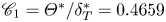 $\mathscr {C}_1=\varTheta ^*/\delta _T^*=0.4659$, where we note that for profile (5.1) our nominal thickness
  $\delta _T^*$ is approximately one fifth of the measured thickness between the positions where the mean velocities are equal to ‘
 $0.01U_J^*$’ and ‘
 $0.99U_J^*$’ (which is the
  $\delta$ given in table 1 of Cavalieri et al. Reference Cavalieri, Rodriguez, Jordan, Colonius and Gervais2013).
Let us concentrate on a CS whose central mode is neutral near  $x_N^*/D^*=2.5$. From figure 3 of Cavalieri et al. (Reference Cavalieri, Rodriguez, Jordan, Colonius and Gervais2013), the dimensional nominal and momentum thicknesses at the neutral position are estimated to be
 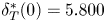 $\delta _T^*(0)=5.800$ mm and
  $\varTheta _N^*=2.702$ mm, respectively. The spreading rate of the momentum thickness is found to be
 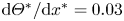 ${{\rm d}\varTheta ^*}/{{\rm d} x^*}=0.03$ by observing the growth of thickness from
  $x^*/D^*=2$ to
  $3$. The critical level is close to lip line
  $r^*=D^*/2$ and so
  $r_c=4.31$. Other dimensionless parameters are
 \begin{equation} {\textit{Re}}=33063,\quad \eta_c^{\dagger}={-}0.02,\quad \alpha=0.391,\quad c=1.221, \end{equation}
and the Strouhal number of the neutral mode at 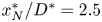 $x_N^*/D^*=2.5$ is
 \begin{equation} St_{D,N}\equiv f^*D^*/U_J^*=\alpha c r_c/(2{\rm \pi})=0.327. \end{equation}
 In order to aid the comparison with experiments, the key relations between the dimensional and normalised variables/quantities are highlighted. The axial position from the nozzle  $x^*/D^*$ is related to the slow axial variable
  $\bar {x}$ in our theory via
 \begin{equation} (x^*-x_N^*)/D^* =\left(c\delta_T^*(0)/D^*\right)\epsilon^{{-}2/5} \bar{x} . \end{equation}
 For a regular critical layer,  $a_+=a_-=a$ (see (3.10)), which is determined when the Rayleigh equation is solved. It follows from (3.22a), (3.24), (3.34) and (3.42) that the leading-order dimensionless axial velocities of the CS at the centrelline
  $r=0$ and at critical level are given by
 \begin{equation} \hat{u}_x(0)=\epsilon\hat{u}_0(r=0)A^{\dagger}(\tau,\bar{x})\mathrm{e}^{\mathop{\rm i}\nolimits\alpha\zeta}+{\rm c.c.}, \end{equation}
 \begin{equation} \hat{u}_x(r_c)=\epsilon\hat{u}_0(r=r_c)A^{\dagger}(\tau,\bar{x})\mathrm{e}^{\mathop{\rm i}\nolimits\alpha\zeta}+{\rm c.c.}, \end{equation}
the latter of which is approximately the axial velocity at  $r^*/D^*=0.5$, since the generalised inflection point is very close to the lip line with the dimensional deviation approximately
  $\eta _c^{\dagger} \delta _T^*=-0.116$ mm (see (3.24) in [II]). In (A5)
 \begin{equation} \hat{u}_0(r=r_c)A^{\dagger}(\tau,\bar{x})={-}aA^{\dagger}(\tau,\bar{x})+(\alpha\bar{U}_c')^{{-}1} \int_{-\infty}^{\sigma\alpha\bar{U}_{1,c}\bar{x}}\tilde{Q}_0(\tau,\bar{x},\bar\eta)\,{\rm d}\bar\eta, \end{equation}
where the integral term can be evaluated analytically using (3.45).
We specify the initial conditions as in the case- ${\mathcal {H}}_W$ (table 2) with the difference frequency
  $St_{D,\nu }=0.02$. It is worth noting that the choice of
  $\epsilon$ does not influence the dynamics or radiation, provided that
  $\epsilon a_0$ is held fixed. We set
  $\epsilon =0.1$ leading to an overall amplitude about
  $0.004$ at the neutral position. The remaining parameters are assigned as:
  $\tilde \lambda =\bar \lambda =(\epsilon ^{6/5}{\textit {Re}})^{-1}$ and
  $\hat \tau _1=\hat \tau _2=0$ since the results are insensitive to the values of
  $\tilde \lambda$ and
  $\hat \tau _i$.
Figure 23 shows the predicted amplitude evolution of the modes with  $St_D=0.4$ and different
  $m$, among which five ring and helical modes are seeded, while others are nonlinearly excited near the neutral position. The overall features are similar to those shown in the main text. Nonlinear effects cause much slower attenuation, which is oscillatory for some components. Comparing the two panels, one notes that the axial velocity along the centreline (which is proportional to the overall amplitude
  $A^{\dagger}$) and the axial velocity on the lip line differ appreciably: the latter peaks and attenuates much later. This is because the shape of the latter, represented by the second and nonlocal term in (A6), undergoes distortion due to the combined leading-order effects of non-equilibrium and non-parallelism in the critical layer. On the centreline the axial velocities of the ring and helical modes are all similar (figure 23a). However, at the lip line, the axial velocity of the ring mode is much smaller than those of the helical modes (figure 23b). This is because the latter are dominated by the second term in (A6), which is associated with three-dimensionality. These differences indicate that appropriate quantitative comparisons have to be made between specific quantities. One may note that the centreline axial velocity amplifies by a factor about 5 over an axial distance of
  $2D^*$, weaker than the growth by a factor of 10 observed in experiment (e.g. figure 28 in Cavalieri et al. Reference Cavalieri, Rodriguez, Jordan, Colonius and Gervais2013). This weaker amplification is due to a rather small, and possibly underestimated, spreading rate
  ${{\rm d}\varTheta ^*}/{{\rm d} x^*}=0.03$ being used. When the latter is increased to
  $0.045$ and the initial amplitudes of the seeded modes are increased by a factor of
  $1.5^{3/2}$, the growth factor over the same axial distance increases to 10 (but the result is not shown). It is impossible to make quantitative comparisons in the compressible regime because nonlinear evolution depends sensitively on the composition of the initial modes, but experiments using controlled excitation have not yet been conducted. The second reason is that the present work focuses on interactions among helical and ring modes, which are of weakly nonlinear form. However, when helical modes are absent or weak, strongly nonlinear self interaction of the ring mode, which is ignored in the present work, becomes important. An appropriate comparison calls for extension of the theory to accommodate this scenario. In the incompressible regime, there have been a few experiments where ring and helical modes were excited in a controlled manner, and a preliminary quantitative comparison was performed in Zhang (Reference Zhang2022), showing encouraging agreement.

Figure 23. Amplitude evolution of the ring/helical modes with the frequency  $St_D=0.4$ represented by the axial velocity on the centreline (a) and the lip line (b). The dashed lines in (a) represent linear evolution.
Figure 24(a,b) shows the acoustic field predicted by the present theory. The sound pressure level (SPL, in dB) in figure 24(a) is defined as
 \begin{equation} \text{SPL}=20\log|\tilde{p}^*/p_{ref}^*|=20\log|(\rho_0^*U_0^{*2})\hat p/p_{ref}^*|, \end{equation}
with the specified reference pressure  $p_{ref}^*=2.0\times 10^{-5}$ Pa. The radiation to the direction
  ${\bar {\varphi }}\approx 60^\circ$ is the strongest. The instantaneous dilatation rate of the low-frequency acoustic field is
 \begin{equation} \boldsymbol{\nabla}\boldsymbol{\cdot}\pmb{u}={-}M\!a^2{\mathcal{D}}_+\tilde{P}, \end{equation}
where  $\tilde {P}$ is given by (6.42). The far field of the dilatation rate is obtained by the stationary-phase method, and the contours are displayed in figure 24(b). Although the flow conditions are different, the main feature of contours resembles that in the DNS results (e.g. figures 11, 16 and 21) of Suponitsky et al. (Reference Suponitsky, Sandham and Morfey2010), which focussed on the lower-frequency sound waves emitted by nonlinear interactions. In particular, the peak radiation direction is about
  $60^\circ$ to the downstream axis, suggesting that this may be a robust character of the envelope radiation.

Figure 24. Contours of the sound pressure (values in contours are in dB) (a) and the instantaneous dilatation rate (b) of the low-frequency acoustic filed.
For the seeded modes with the amplitudes specified, the overall intensity of the low-frequency sound waves is in the range of  $90\sim 100$ dB along
  $r^*/D^*=35$, which is comparable to that measured for the component of the lowest frequency (
 $St_D=0.1$) (see figure 8 in Cavalieri et al. Reference Cavalieri, Jordan, Colonius and Gervais2012). However, discrepancies from the experimental measurements exist. For example, the overall acoustic directivity in the latter peaks at polar angles between
  $20^\circ \sim 40^\circ$, significantly lower than
  $60^\circ$. Possible reasons are now discussed with references to the limitation of the present theory. The noise measured in the frequency band of
  $0.2\leqslant St_D\leqslant 0.9$ is, as discussed in our previous work ([II]), contributed by CS in (a) the developed (see Wu & Huerre Reference Wu and Huerre2009; [II]), (b) the near-nozzle (the present investigation) and (c) the very-near-nozzle (see § 4.4 and Zhang & Wu Reference Zhang and Wu2023b) regions, and possibly by fine-scale turbulence also. Moreover, represented by a wavepacket, a CS may emit sound waves by (at least) two mechanisms (Zhang & Wu Reference Zhang and Wu2023a): a linear mechanism, through which a spatially modulated wave emits sound waves of the same frequencies as the fundamental and its harmonics (Tam & Morris Reference Tam and Morris1980; Cavalieri et al. Reference Cavalieri, Jordan, Colonius and Gervais2012; Zhang & Wu Reference Zhang and Wu2023b), and a nonlinear mechanism (Wu & Huerre Reference Wu and Huerre2009; Suponitsky et al. Reference Suponitsky, Sandham and Morfey2010; [I]; [II]), through which a spatially and temporally modulated wavepacket generates sound waves in a band of frequencies much lower than the central frequency of the CS. These linear and nonlinear mechanisms operate simultaneously in practice, emitting noise of comparable intensity for a CS of wavepacket with a moderate amplitude. The relatively high- and low-frequency noise dominates the near axis and sideline directions, respectively. The present work has considered only the nonlinear mechanism pertinent only to a CS in a near-nozzle region where the potential core is about to disappear. For an appropriate comparison with experimental measurements, further theoretical development is needed. Firstly, it is necessary to account for also the sound waves radiated by the CS in the developed region through the linear mechanism (cf. Zhang & Wu Reference Zhang and Wu2023a). With this portion of noise included, it is expected that the peak radiation angle of the overall noise would be smaller than
  $60^\circ$. Secondly, for improved accuracy and/or convenience of application it is desirable to construct a unified or composite theory that describes the nonlinear dynamics and acoustic radiation of CS in all (very-near-nozzle, near-nozzle and the fully developed) regions (cf. Zhang & Wu Reference Zhang and Wu2023b). Efforts on both fronts are being made in our ongoing projects.


