


1. Introduction
Glacier mass change holds global significance as it has far–reaching impacts on sea level, ecosystem hydrology, and the water requirements of communities downstream (Milner and others, Reference Milner2017; Brighenti and others, Reference Brighenti2019; Zemp and others, Reference Zemp2019). Glacier melt was the largest contributor to sea level rise over the 20th century, and is projected to remain a significant contributor throughout the 21st century (Marzeion and others, Reference Marzeion2017; Slangen and others, Reference Slangen2017; Farinotti and others, Reference Farinotti, Round, Huss, Compagno and Zekollari2019; Frederikse and others, Reference Frederikse2020). Moreover, glaciers’ water storage capacity makes their monitoring and prediction crucial to water resources management (Jansson and others, Reference Jansson, Hock and Schneider2003; Förster and van der Laan, Reference Förster and van der Laan2022; Ultee and others, Reference Ultee, Coats and Mackay2022). To predict glacier mass loss for the 21st century, a ‘top–down’ approach is typically used. Top–down refers to the cascading down of information, resulting in a system response. Glacier models are forced with regional climates, directly or indirectly derived from General Circulation Models (GCM), to simulate glacier mass evolution under imposed scenarios, see e.g. Hock and others (Reference Hock2019) for a comprehensive overview. However, much of the manifestation of specific climate change scenarios is shaped by socioeconomic and political development, introducing uncertainties into scenario projections and impact (Reilly and others, Reference Reilly2001; Kemp and others, Reference Kemp2022). Scenarios start to diverge significantly mid 21st century, after which they dominate the uncertainty in glacier model projections (Hinkel and others, Reference Hinkel2019; Marzeion and others, Reference Marzeion2020). On the near term, individual models nonetheless produce individual results with the same scenario. This stems from a combination of internal variability and climate model differences and still adds uncertainty to results (Marotzke, Reference Marotzke2019).
The uncertainty from top–down approaches can cause difficulties in the interpretation and communication of results for decision–making processes and science communication (Girard and others, Reference Girard, Pulido-Velazquez, Rinaudo, Pagé and Caballero2015). Consequently, there has been a growing effort over the past decade to better integrate top–down and so–called ‘bottom–up’ approaches, complementing each other's insights (Bhave and others, Reference Bhave, Mishra and Raghuwanshi2014; Conway and others, Reference Conway2019). Bottom–up here refers to a focus on sensitivity or vulnerability of a system, accounting for a range of potential climate changes, regardless of specific scenarios and their inherent uncertainties (Guo and others, Reference Guo, Westra and Maier2017; Culley and others, Reference Culley, Maier, Westra and Bennett2021). In the field of hydrology and water resources management, especially in addressing extreme events such as floods and droughts, bottom–up approaches, using a number of scenario–neutral methods, have gained traction (e.g. Prudhomme and others, Reference Prudhomme, Wilby, Crooks, Kay and Reynard2010; Guo and others, Reference Guo, Westra and Maier2018; Keller and others, Reference Keller, Rössler, Martius and Weingartner2019; Beylich and others, Reference Beylich, Haberlandt and Reinstorf2021). A central aspect of these studies involves identifying and focusing on the climate variables to which the system is most sensitive (Girard and others, Reference Girard, Pulido-Velazquez, Rinaudo, Pagé and Caballero2015; Guo and others, Reference Guo, Westra and Maier2017). The main benefit of the studies lies in the simple implementation and rapid appraisal of results (Prudhomme and others, Reference Prudhomme, Wilby, Crooks, Kay and Reynard2010). In glaciology, bottom–up approaches often encompass the analysis of glacier sensitivity to climate change: the mass balance change for a given temperature or precipitation change (Anderson and others, Reference Anderson2010). This knowledge is essential to develop and aid the traditional top–down modeling of glacier mass change. Multiple studies of glacier sensitivity have been conducted over the past few decades, highlighting the impact of geographical location and glacier geometry on sensitivity (Oerlemans and Fortuin, Reference Oerlemans and Fortuin1992; De Woul and Hock, Reference De Woul and Hock2005). These studies generally focus on one or few, often well–documented glaciers, such as Anderson and others (Reference Anderson2010) and Kumar and others (Reference Kumar, Negi and Kumar2020). They form important initial knowledge for e.g. larger–scale regional studies (top–down) and assessment of climate change hazard risk (direct use of bottom–up results) (De Woul and Hock, Reference De Woul and Hock2005; Knight and Harrison, Reference Knight and Harrison2023).
The current study presents a bottom–up, scenario–neutral approach with the following aims: (1) to present a simple method for sensitivity analysis of every global glacier, (2) to show the integration with a top–down approach and, (3) to propose method applications to benefit decision–making and communication needs regarding glacier response to climate change. As a proof–of–concept, we focus on four case–study glaciers for which observed mass balance data and previous sensitivity studies exist. We model mass balance using a temperature index model and estimate both overall and seasonal glacier sensitivity, presented visually and numerically. The visual display method is in the form of response surfaces: two–dimensional planes which map a system's response to a variation in the parameters or variables displayed on the axes. In this case, the axes represent the changes in temperature and precipitation relative to a baseline. Visualization through response surfaces is common in scenario–neutral approaches, as seen in for example Culley and others (Reference Culley2016) and Sauquet and others (Reference Sauquet, Richard, Devers and Prudhomme2019). The numerical representation is through a glacier sensitivity index (GSI). We integrate the scenario–neutral approach with a top–down approach by superimposing temperature and precipitation from four Coupled Model Intercomparison Project Phase 6 (CMIP6) models, driven with four Shared Socioeconomic Pathways (SSP), onto the response surfaces. Finally, we propose the use and interpretation of scenario–neutral results for decision–making practices and climate science communication.
2. Case study sites
To highlight the differences in climate sensitivity between glaciers, we look at four glaciers in different climatic zones: Hintereisferner (Austria), Austre Brøggerbreen (Svalbard, Norway), Abramov Glacier (Kyrgyzstan) and Peyto Glacier (Canada) (Fig. 1). All four glaciers are World Glacier Monitoring Service (WGMS) reference glaciers and have been the subject of numerous glaciological studies throughout the past decades, (e.g. Young, Reference Young1981; Dirmhirn and Trojer, Reference Dirmhirn and Trojer1955; Oerlemans and Fortuin, Reference Oerlemans and Fortuin1992; Kuhn and others, Reference Kuhn1999; Etzelmüller and others, Reference Etzelmüller2000; Denzinger and others, Reference Denzinger2021). The availability of data and previous work to understand these glaciers, including their sensitivity, make them ideal proof–of–concept sites for our approach.

Figure 1. Glacier outlines according to the (RGI Consortium, 2017), from top left in clockwise order: Hintereisferner (Austria), Austre Brøggerbreen (Svalbard, Norway), Abramov Glacier (Kyrgyzstan) and Peyto Glacier (Canada). Inset shows location of the map in their respective country, labels depicting state and/or country codes.
2.1 Hintereisferner
Hintereisferner (46.79°N, 10.77°E), located in the Ötztal Alps in Austria, is a clean–ice valley glacier. Its 2011 area was approximately 6.8 km2, about 15% smaller than in 2001 (Klug and others, Reference Klug2018). Its elevation ranges from 2430 m a.s.l. at the terminus (in the outline used here, RGI Consortium, 2017) to 3661 m a.s.l. (Wijngaard and others, Reference Wijngaard2019). The glacier is located in the ‘inner dry Alpine zone’, one of the driest places in the European Alps. At the meteorological station in Vent, located 8 km west of the glacier, at 1900 m a.s.l., annual mean precipitation is approximately 750 mm a−1 (1987–2016) and annual mean temperature is approximately 3$^\circ$ C (Klug and others, Reference Klug2018). Most years, annual mean precipitation at the glacier is considerably higher than in Vent, up to double the amount (Fischer, Reference Fischer2013). This is confirmed by precipitation gauge measurements at the glacier and in Vent, see Strasser and others (Reference Strasser2018).
2.2 Austre Brøggerbreen
Austre Brøggerbreen (78.89$^\circ$ N, 11.84$^\circ$
 E) is a valley/cirque glacier located on the archipelago of Svalbard, Norway. The glacier has an area of 6.1 km2 (2012), and ranges in elevation from 50 to 650 m a.s.l. (Bruland and Hagen, Reference Bruland and Hagen2002; RGI Consortium, 2017). Austre Brøggerbreen has lost over 50% of its area since 1936. It is situated in a High Arctic climate, characterized by low temperatures and relatively low precipitation, though the meteorological stations in Longyearbyen and Ny–Ålesund, the latter approximately 4 km from the glacier, show the local climate to be warm compared to other locations between 70 and 80$^\circ$
 N (Eckerstorfer and Christiansen, Reference Eckerstorfer and Christiansen2011). The mean annual air temperature, measured at the equilibrium line altitude (approximately 300 m a.s.l.), was $-8.0^\circ$
 C in the period 1969-1990. In Ny–Ålesund, the mean annual temperature was $-5.2^\circ$
 C from 1981–2010, an increase from $-6.3^\circ$
 C in the period 1969–1990, due to Arctic amplification (Førland and others, Reference Førland, Benestad, Hanssen-Bauer, Haugen and Skaugen2011; López-Moreno and others, Reference López-Moreno, Boike, Sanchez-Lorenzo and Pomeroy2016). Mean annual precipitation in Ny–Ålesund was 385 mm a−1 and 427 mm a−1 for the periods 1961–1990 and 1981–2010, respectively (Førland and others, Reference Førland, Benestad, Hanssen-Bauer, Haugen and Skaugen2011).
2.3 Abramov Glacier
The Abramov Glacier (39.60$^\circ$ N, 71.55$^\circ$
 E) is a valley glacier in the Koksu Valley, Pamir–Alay range, in Kyrgyzstan. It has an area of 24 km2 and spans an elevation range of 3650 to 5000 m a.s.l. (in 2015) (Kronenberg and others, Reference Kronenberg, Machguth, Eichler, Schwikowski and Hoelzle2021). Between 1975 and 2015, the glacier has lost about 5% of its area, and retreated approximately 1 km (Barandun and others, Reference Barandun2015). The Abramov Glacier is located in a continental climate. Mean annual temperature recorded at the glacier meteorological station (3837 m a.s.l.) was $-4.1^\circ$
 C for the period 1968–1998 (Kronenberg and others, Reference Kronenberg2022). Mean annual precipitation was 750 mm a−1 from 1968–1998, with maximum precipitation occurring from March to May (Kronenberg and others, Reference Kronenberg2022).
2.4 Peyto Glacier
Peyto Glacier (51.67$^\circ$ N, –116.54$^\circ$
 E) is a mountain glacier located in Banff National Park, Canada. With its continued observation, Peyto Glacier is considered an important ‘index glacier for the region’ (Kehrl and others, Reference Kehrl, Hawley, Osterberg, Winski and Lee2014). It had an area of 9.7 km2 in 2006, and its elevation ranges from 2647 m a.s.l. to 3032 m a.s.l. (Kehrl and others, Reference Kehrl, Hawley, Osterberg, Winski and Lee2014; Pradhananga and others, Reference Pradhananga2021). The glacier has continuously been losing mass since at least the 1920s. It is located in a continental climatic regime, characterized by relatively low precipitation inputs and large variability in temperature (Young, Reference Young1981). Temperature records from a meteorological station on the glacier, set up and documented by Pradhananga and others (Reference Pradhananga2021), show that the daily average temperature varied between $15 ^\circ$
 C and $-30^\circ$
 C during the period 2013–2018. Records from the closest meteorological station at Bow Summit, approximately 15 km from the glacier, show that total annual precipitation varies between 600 and 1300 mm a−1 (Mukherjee and others, Reference Mukherjee2022).
3. Data and methods
3.1 The open global glacier model
The Open Global Glacier Model (OGGM) is an open–source, modular, numerical model framework with a glacier–centric approach, developed by Maussion and others (Reference Maussion2019). It is used to model global past and future glacier evolution. For the current study, we only use OGGM's mass balance model (v. 1.6.0). When using the default pre–processing capabilities, the Randolph Glacier Inventory (RGI) v. 6 provides the glacier outlines used in OGGM, while the digital elevation models are selected per glacier from various available datasets, depending on the region. For the current study, the digital elevation models stem from NASADEM and COPDEM (Crippen and others, Reference Crippen2016; Fahrland and others, Reference Fahrland, Jacob, Schrader and Kahabka2020, respectively).
As climate input, we use time series of temperature and precipitation from the Climatic Research Unit (CRU) TS v4.01 dataset (Harris and others, Reference Harris, Jones, Osborn and Lister2014). The time series are then downscaled to the CRU 1961–1990 CE climatology (New and others, Reference New, Lister, Hulme and Makin2002), which contains elevation data, using the delta method (Ramírez Villegas and Jarvis, Reference Ramírez Villegas and Jarvis2010; Getahun and others, Reference Getahun, Zewdu and Mekuria2021). This step is necessary because the time series do not contain altitude information, which is needed to compute the temperature at a given glacier elevation.
The temperature and precipitation time series are then applied in a temperature index model, in which monthly mass balance is calculated according to:

Here, m i(z) represents the monthly mass balance at altitude z, $P_i^{solid}$ is the solid precipitation, calculated from the total monthly precipitation, according to a temperature threshold, and μ* is the temperature sensitivity parameter. The temperature threshold used to distinguish between rain and snow assumes that all precipitation is solid when the monthly mean temperature is below 0$^\circ$
 C and all precipitation is liquid when the temperature is above 2$^\circ$
 C. Between these two temperatures, it is linearly interpolated. p f is a multiplicative precipitation correction factor and t b is a temperature bias. The temperature lapse rate is assumed to be $-6.5^\circ$
 C km−1 and the threshold temperature T melt for melt is assumed to be $-1^\circ$
 C.
C.
The current study makes use of the pre–processed OGGM directories, for which the temperature sensitivity parameter, the precipitation factor and the temperature bias are calibrated to match each glacier's observed geodetic mass balance from the dataset by Hugonnet and others (Reference Hugonnet2021). The parameter values from the pre–processed directories are used in the baseline (unperturbed) run of each glacier in this study and can be found in Table 1. For an in–depth description of OGGM, its calibration, characteristics and workflow, please refer to Maussion and others (Reference Maussion2019) or https://docs.oggm.org.
Table 1. Parameter values during the unperturbed run and mean glacier sensitivity index GSI T, for all four glaciers
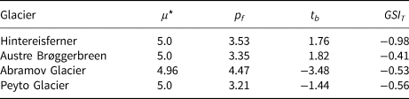
Units are as follows: temperature sensitivity parameter μ* (kg m−1 day−1 K−1), precipitation p f is a multiplicative factor without a unit, temperature bias t b ($^\circ$ C) and glacier sensitivity index GSI T (m w.e. a$^{-1}{}^\circ {\rm C}^{-1}$
 ).
).
3.2 CMIP6 models
For the integration with a top–down approach, we analyze temperature and precipitation from four GCMs, forced with four scenarios, obtained from CMIP6 archived model output. These models are FGOALS3, MPI–ESM1, EG–Earth 3 and NorESM2. We use the r1i1p1f1 realization of all models. In order to obtain datasets spanning 2000–2100, we merge GCM output from the CMIP6 experiment ‘historical’, which spans the years 1850–2015, and GCM output under four SSPs (2015–2100): SSP 1–2.6, 2–4.5, 3–7.0 and 5–8.5 (O'Neill and others, Reference O'Neill2016). The SSPs are updated versions of the previous Representative Concentration Pathways (RCP) (van Vuuren and others, Reference van Vuuren2011). SSPs are driven by emissions and land–use scenarios and refer to climate mitigation, adaptation and impacts. SSP 1–2.6, updated RCP 2.6, refers to a level of radiative forcing of 2.6 Wm−2 in 2100 and represents the low end of the future forcing pathways. SSP 2–4.5 (updated RCP 4.5) refers to 4.5 Wm−2 as representing the medium level. SSP 3–7.0 is a newly added level at the high end of the range referring to 7 Wm−2 radiative forcing in 2100. SSP 5–8.5 (updated RCP 8.5), representing the high end of the future pathways, refers to 8.5 Wm−2.
3.3 Unperturbed baseline climate simulation
In order to create a set of baseline—unperturbed – results, we force the calibrated OGGM mass balance model with the CRU baseline climate described above, 1985–2015. From here on, these runs are referred to as ‘unperturbed’. We compute mass balances with fixed glacier geometries, which correspond to the outline at the glacier's RGI dates: Hintereisferner—2003; Austre Brøggerbreen—2007; Abramov Glacier—2000; Peyto Glacier—2004. To ascertain that our baseline results are reliable and the method is transferable to glaciers with little or no observed data, we validate the results against the WGMS observed mass balance data (WGMS, 2022). We assess skill via the calculation and analysis of the mean error, mean absolute error and Pearson correlation. For the mean error, we subtract observed mass balance from modeled mass balance in the same year, for each glacier, over the period 1985–2015 (N = 107, because of a lack of observations for the Abramov Glacier from 2000–2012). The mean absolute error is calculated for each glacier based on the absolute differences between the observed and modeled mass balances. The mean absolute error, as it does not take the direction of error into account, provides more information about the magnitude of the discrepancy between modeled and observed values. Finally, we calculate the Pearson correlation coefficient, as a a measure of agreement between simulated and observed mass balance.
3.4 Scenario–neutral approach
Scenario–neutral climate change studies generally describe the effects of climate attribute changes on a system. In such studies, these attributes can change independently, and the impact is not influenced by timing or other variables affecting the system. In our particular case however, because of the impact of temperature on the phase of precipitation, the variables are not fully independent. The disproportionate impact of temperature needs to be taken into account when assessing the magnitude of the impact of precipitation change. However, precipitation also has an isolated effect on mass balance through variations in amount (see Eqn (1)). This is cause for a separate axis in the response surfaces, making the method suitable for mass balance studies.
We analyze the impact of changes in precipitation and temperature, relative to the unperturbed run. We do this in a multitude of combinations, for example a 20$\%$ increase in precipitation and no change in temperature, a 10$\%$
 decrease in precipitation and $5^\circ$
 C increase in temperature, or both attributes remaining at baseline in summer, while changing in winter. These changes are not associated with a particular climate change scenario. The magnitude of the response is a means to assess and convey system sensitivity.
Glacier mass balance is, in reality, also influenced by changes in glacier geometry. This subsequently impacts glacier volume and area. Our simple, fixed geometry approach allows the advantage of modeling glacier response to climate attribute changes under which the real–world glacier would have significantly changed geometry or vanished entirely. For a smaller glacier, the mass balance would be less negative, as a result of changes in geometry. The fixed geometry approach produces mass balance that is termed ‘reference surface mass balance’ by Elsberg and others (Reference Elsberg, Harrison, Echelmeyer and Krimmel2001), which has a more clear relationship with changes in climate than mass balance computed with changing glacier geometry. For each of the four glaciers in our case study, we employ the following steps towards construction of a scenario–neutral space, outlined in Culley and others (Reference Culley, Maier, Westra and Bennett2021):
(1) Selection of Climate Attributes: Temperature and precipitation are the climate attributes selected for our approach. Our choice of climate attributes is forced by the selection of a temperature index model for the calculation of the system response: OGGM's mass balance model, which uses monthly time series of precipitation and temperature as input. This simple method makes it possible to apply the method on a large scale and to regions with a low observational density.
(2) Development of Perturbed Attribute Values: The boundaries and incremental changes of the selected climate attributes are chosen. Since we consider the CMIP6 SSP scenarios until 2100 in the integration of top–down and bottom–up approaches, we use temperature and precipitation from these projections as boundary guidelines. To calculate boundaries for the perturbation of mean annual temperature and annual precipitation, we calculate the difference between the mean values from OGGM baseline climate CRU 1985–2015 and EC–Earth SSP585 values 2070–2100 at the glacier locations. The largest temperature difference is found for Austre Brøggerbreen, with a mean annual temperature over the unperturbed period of $-7.2^\circ$
 C and of $3.6^\circ$C during 2070–2100. To include this scenario in our boundaries, we apply a perturbation of up to $+ 11^\circ$C. For the lower temperature boundary, we include a temperature perturbation of $-3^\circ$C, to assess the impact of cooling. For total annual precipitation, we use a multiplicative factor rather perturbing by fixed amounts. This takes the large differences in precipitation between the glacier locations into account, making comparison easier. Also here, we find the largest differences from the baseline in SSP585, and in this case for Hintereisferner and Peyto Glaciers. For Hintereisferner, we see a decrease of 10%, from 1480 mm per year to 1310 mm per year between the unperturbed period and 2070–2100. For Peyto Glacier, we see an increase of 48% in precipitation, from 1148 mm per year to 1709 mm per year. To include these scenarios, we apply boundaries of –20% to +50% in precipitation.
We apply the same method to establish perturbation boundaries for the period 2010–2040, which we look at in the top–down integration. This ensures all CMIP6 scenarios and models are represented within the response surfaces. We note that the boundaries are chosen to incorporate the various SSP scenario ranges, rather than to represent the bounds of plausible changes.
(3) Generation of Perturbed Time Series: To reflect these perturbations in our climate attribute time series, we make use of the temperature bias t b and the precipitation factor p f, see Eqn (1). We adjust the temperature bias from the unperturbed run with a specified additive temperature anomaly in $^\circ$
C, according to the increments on the response surface axes, referred to as the temperature perturbation. Depending on the glacier, we use increments of $0.5^\circ$C or $1^\circ$C. We adjust precipitation factor p f with a multiplicative precipitation anomaly, referred to as the precipitation perturbation, in increments of 5% to 10%, depending on the glacier. Also here, the percentages indicated are relative to the unperturbed run. To calculate seasonal sensitivity, during either winter (October–March) or summer (April–September) the climate forcing of one season is that of the unperturbed run, while the climate forcing for the other season is perturbed as described above.(4) Assessment of System Response: We force OGGM for the period 1985–2015, with the baseline climate and with each incrementally perturbed 30–year time series. This results in an annual mass balance time series over the 30–year time period. From this, we calculate the mean annual mass balance over the time period, which is depicted in the response surface.


3.5 Glacier sensitivity index
To support the visual component of our method, we also calculate a glacier sensitivity index (GSI). This allows comparison with calculated glacier sensitivities from the literature. The GSI builds upon the idea by Oerlemans and Reichert (Reference Oerlemans and Reichert2000) that mass balance can be related to precipitation and temperature with a sensitivity characteristic. The GSI is calculated per glacier, for perturbations in temperature only. The sole influence of precipitation would be more difficult to quantify in a sensitivity characteristic, as its phase is dependent on temperature.
We only calculate the GSI in instances where temperature is perturbed and precipitation is not, to isolate the temperature perturbation's impact. The calculation is done as follows:

in which m k and m ref,k represent the mass balance in year k of the perturbed run, and year k of the unperturbed run. t p refers to the temperature perturbation. GSI T is calculated annually and has the unit of m w.e. a$^{-1}{}^\circ {\rm C}^{-1}$ .
.
The magnitude and the inter–annual variability of the glacier sensitivity index values represent the influence of temperature on mass balance, representing system response. The more negative the GSI, the larger the influence of a temperature perturbation on the system. The larger the variability, the less consistent the influence of temperature changes on the system is.
3.6 Top–down method integration
As a very simple example of combining scenario–neutral methods with a traditional top–down approach, we analyze four CMIP6 models and SSP scenarios, outlined in section CMIP6. For each model and scenario, we calculate the mean annual temperature and annual precipitation over 30 year periods, 2010–2040 and 2070–2100, at the glacier location. The differences between these values and the mean baseline time series are then calculated. These values represent the climate attribute change in the model iteration, relative to the baseline. The results determine the position on the axes and are superimposed onto the response surface. This method is commonly applied in combination with scenario–neutral approaches, see for example Prudhomme and others (Reference Prudhomme, Wilby, Crooks, Kay and Reynard2010) and Sauquet and others (Reference Sauquet, Richard, Devers and Prudhomme2019). The superimposed values serve as an initial assessment of the differences between models and scenarios in the context of the system response, before starting computationally expensive simulations.
4. Results
4.1 Unperturbed run
For the period 1985–2015, we compare modeled mass balances from the unperturbed run to observed mass balances from the WGMS dataset WGMS (2022). We calculate the model performance measures outlined in Table 2. Both individually and averaged over all four glaciers, we see good agreement between modeled and observed mass balances, with the exception of the Abramov Glacier. Averaged over all four glaciers, the mean error is 0.26 ± 0.51 m w.e. a−1 and the mean absolute error is 0.48 ± 0.34 m w.e. a−1, affected by the large errors for the Abramov Glacier. For the other three glaciers, the agreement between observed and modeled mass balance is satisfactory (mean error less than 0.2 m w.e. a−1). Overall, the errors are comparable to the error values Eis and others (Reference Eis, Van der Laan, Maussion and Marzeion2021) find for the validation of their mass balance reconstruction of all reference glaciers. Figure 2 shows that the cumulative mass balances, observed and modeled, match well, though the model underestimates the mass balance, for Hintereisferner and Austre Brøggerbreen in particular.
Table 2. Statistics comparing observed and modeled mass balances from the OGGM unperturbed run, for all four glaciers
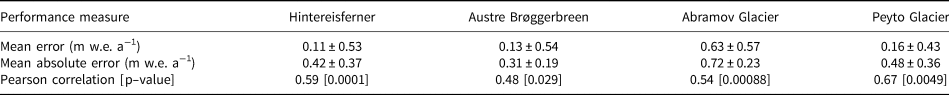
All metrics and standard deviations of the metrics are mean values per glacier, calculated over each set of metrics. For the Pearson correlation, the p–values have been added in square brackets. The p–values, all below 0.05 indicate that all Pearson correlations are statistically significant.
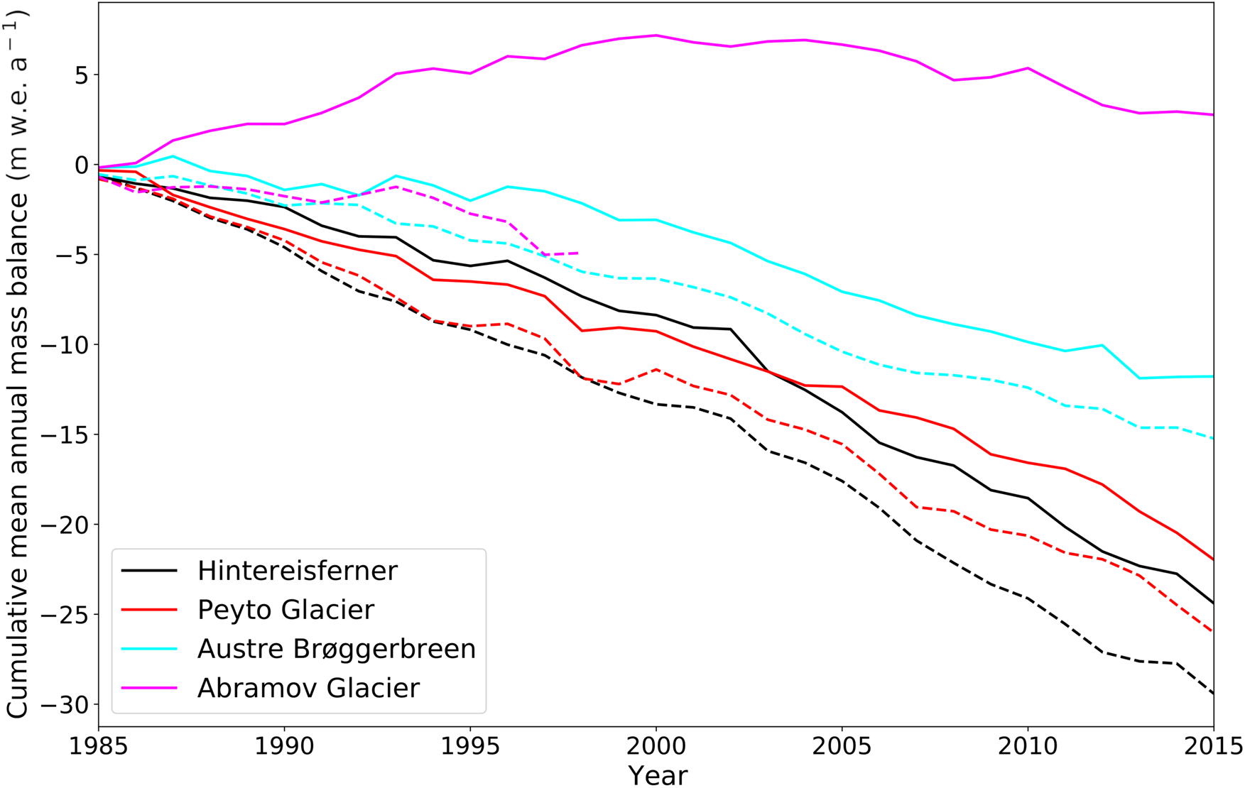
Figure 2. Cumulative mass balance over the period 1985–2015 as simulated with OGGM for the unperturbed run (solid lines), and observed (dashed lines) (WGMS, 2022).
The underestimation of the mass balance for all glaciers can result from the differences between the two datasets of observed mass balance, used in this study. For the development of the pre-processed directories, OGGM is calibrated against geodetic mass balance observations from Hugonnet and others (Reference Hugonnet2021), whereas here, we compare the results from the unperturbed run against the WGMS observed mass balance dataset (WGMS, 2022). Van der Laan and others (Reference van der Laan, Vlug, Scaife, Maussion and Förster2024) compare the two datasets where they overlap, meaning the glacier is included in the geodetic dataset and has annual data in the WGMS dataset. This is the case for 67 glaciers over the period 2000–2019. The mean difference, subtracting mean annual geodetic mass balance from mean annual WGMS mass balance, is –0.11 m w.e. a−1, indicating a systematic difference between the two datasets. This difference is similar in magnitude to the differences between our observed and simulated values for three of the four glaciers, see Table 2. The WGMS mass balances being more negative on the whole can explain the mismatch with a simulation from a model calibrated against the geodetic data. This highlights the potential difficulty in working with pre–calibrated parameters and determining the suitability of a parameter set against an independent dataset.
However, the large errors for the Abramov Glacier cannot be explained through dataset differences alone. For the Abramov Glacier, 13 of the 30 observed years are missing, so it is not possible to show the goodness of fit in terms of cumulative mass balance over the whole period. This is why the years 2011–2015, though observations exist, are removed from Fig. 2. The work by Kronenberg and others (Reference Kronenberg2022) finds that the mass balance of the Abramov Glacier has been predominantly negative since the 1970s. Comparing our results with this study confirms that the positive modeled mass balance in the unperturbed run is incorrect. This is also reflected in the large mean error of 0.63 m w.e. a−1), calculated against the WGMS observed data. The simulated positive mass balance results from the parameter values used for the unperturbed run (Table 1). These parameter values are calibrated for the pre–processed directories to match geodetic mass balance over the reference period 2000–2019 Hugonnet and others (Reference Hugonnet2021). This observed mass balance, of −0.24 m w.e. a−1, is indeed matched when simulating only the period 2000–2019. For our study period of 1985–2015 however, these parameter values cause a systematic cold bias. The calibrated temperature bias, used for the unperturbed run, is $-3.5^\circ$ C. This temperature bias is subtracted from the temperature forcing, which leads to a mean annual forcing temperature of $-6.2^\circ$
 C, significantly lower than the observed mean annual temperature at the Abramov Glacier ($-4.1 ^\circ$
 C in 1968–1998 Kronenberg and others, Reference Kronenberg2022). This cold model bias causes an overestimation of the amount of precipitation that falls as snow, and an underestimation of melt. The result is an erroneously positive mass balance. OGGM offers the option to re-calibrate for each glacier, against a variety of datasets, to ensure a better fit for the user's needs. However, doing this for the current study would take away from the main benefit of our method: ease and speed of use for initial studies, for any glacier. Making the choice between re–calibration versus using the out–of–the–box pre–processed directories emphasizes the challenge of balancing complexity and wide applicability.
4.2 Scenario–neutral approach
4.2.1 Overall sensitivity
As outlined above, we generate response surfaces according to the four steps suggested in Culley and others (Reference Culley, Maier, Westra and Bennett2021). Using our defined boundaries, this results in a response surface over the period 1985–2015 for Hintereisferner, Austre Brøggerbreen, Abramov Glacier and Peyto Glacier (Fig. 3). We present our results within the context of observed data and results from the literature on their climate and sensitivities.

Figure 3. Response surfaces for (a) Hintereisferner, (b) Austre Brøggerbreen, (c) Abramov Glacier and (d) Peyto Glacier, resulting from the fully perturbed time period 1985–2015. Mass balance values represent the annual mean over the 30–year time period. For comparison purposes, the color bars are unified and the transition blue–orange is centered at 0 m w.e. a−1.
Hintereisferner responds most sensitively to the changes in climate attributes. In the unperturbed run, mean annual mass balance is −0.97 m w.e. a−1. At the far end of the perturbation boundaries, with a decrease in precipitation of 20% and temperature increase of 11$^\circ$ C, mean annual mass balance goes down to −14.2 m w.e. a−1. Increases in precipitation markedly affect mass balance in the realm of a temperature perturbation of $-2^\circ$
 C to $2^\circ$
 C, after which precipitation ceases to have an effect. This is likely due to a removal of accumulation from the mass balance Eqn (1), entirely, as also winter temperatures are above the threshold at which precipitation falls as snow. The fact that the Hintereisferner has the highest amount of annual precipitation confirms the ideas discussed in Meier (Reference Meier1984); Oerlemans and Fortuin (Reference Oerlemans and Fortuin1992) and Oerlemans and Reichert (Reference Oerlemans and Reichert2000) that sensitivity goes up with precipitation amount, and that generally, glaciers with a higher mass turnover are more sensitive. Hintereisferner's high sensitivity is also conveyed through having the most negative GSI T (−0.84 m w.e. a$^{-1}{}^\circ {\rm C}^{-1}$
 —−1.36 m w.e. a$^{-1}{}^\circ {\rm C}^{-1}$
 ). The numbers for the GSI T are in line with the observed temperature sensitivity for the glacier calculated by Fischer (Reference Fischer2010) after 1979, which ranges between −0.38 m w.e. a$^{-1}{}^\circ {\rm C}^{-1}$
 and −1.54 m w.e. a$^{-1}{}^\circ {\rm C}^{-1}$
 .
.
For Austre Brøggerbreen, Elagina and others (Reference Elagina2021) find a temperature sensitivity of −0.49 m w.e.a$^{-1}{}^\circ {\rm C}^{-1}$ , which is exactly in the GSI T range we find for the glacier: between −0.33 m w.e. a$^{-1}{}^\circ {\rm C}^{-1}$
 and −0.57 m w.e. a$^{-1}{}^\circ {\rm C}^{-1}$
 . Its sensitivity to precipitation decreases with increasing temperature, becoming solely impacted by temperature at a perturbation of 6$^\circ$
 C (see Fig. 4). This points to the detrimental effect the process of Arctic amplification will likely have on the glacier's mass balance in the 21st century. The likelihood and magnitude of Arctic amplification for the region is analyzed by van Pelt and others (Reference van Pelt, Schuler, Pohjola and Pettersson2021), who find a temperature increase of 6–7$^\circ$
 C and 45$\%$
 increase in precipitation when comparing 1971–2001 observations of Svalbard climate to global and regional projections for Svalbard in 2071–2101.
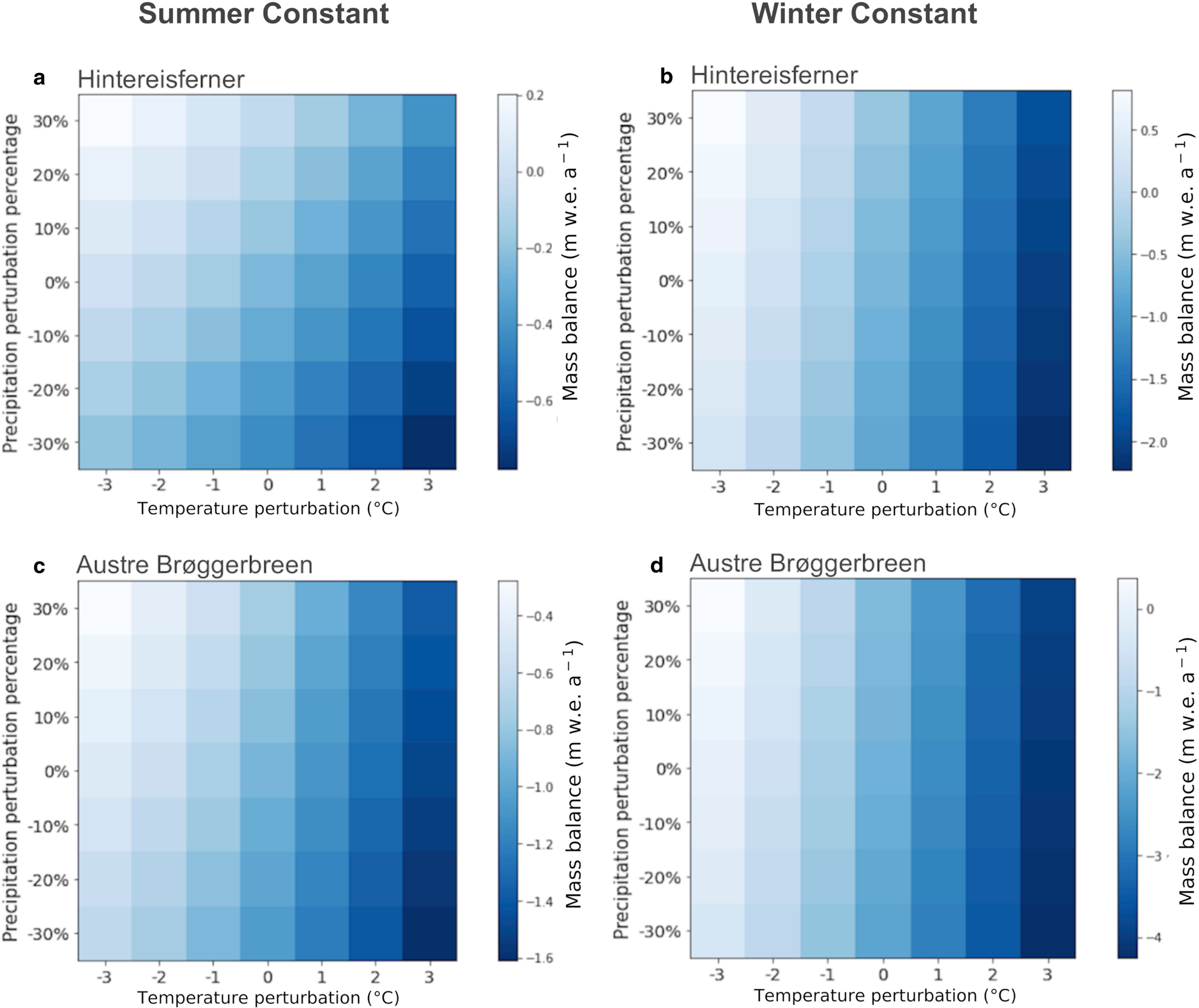
Figure 4. Response surfaces for Hintereisferner (a) and (b) and Austre Brøggerbreen (c) and (d), resulting from the seasonally perturbed time period 1985–2015. The word ‘constant’ at top of the figure refers to a perturbation of 0 for that season in all years. Mass balance values represent the annual mean over the 30–year time period. The summer contribution to mass balance for ‘summer constant’ is −0.98 m w.e. a−1 for Austre Brøggerbreen (a) and −1.94 m w.e. a−1 for Hintereisferner (c). For ‘winter constant’, the winter contributions to mass balance are 0.43 m w.e. a−1 (b) and 0.16 m w.e. a−1 (d). For clear contrast of the colors, and thus of the differences per season and glacier, the color scales are not unified, so please note.
Of the four glaciers, the Abramov Glacier has the lowest sensitivity to the changes in climate attributes, with a mean annual mass balance of −6.8 m w.e. a−1 at the far end of the perturbations, compared to −14.2 m w.e. a−1 for the Hintereisferner. The cold bias in the model, when applied to the Abramov Glacier, causes an erroneously positive mass balance in the unperturbed run. This results in an underestimation of the glacier's sensitivity to temperature perturbations, as it takes much larger perturbations, relative to the unperturbed run, to reach conditions under which mass balance is negative. The cold model bias also causes an overestimation of sensitivity to precipitation, due to a larger fraction of precipitation falling as snow. In spite of this overestimation, like the other three glaciers, Abramov Glacier is sensitive to temperature over precipitation, especially as temperatures increase (Fig. 3). This matches findings by Barandun and others (Reference Barandun2015), who note that the Abramov Glacier's sensitivity to summer temperatures is critical to the glacier's mass loss. A study by Wortmann and others (Reference Wortmann2022) points out that the climate in the glacierized basins of Kyrgyzstan is predicted to become warmer and wetter in the future. But with its low sensitivity to precipitation, this means that even as the climate in Kyrgyzstan gets wetter, it will likely have little positive impact on the glacier's mass balance.
Finally, Peyto Glacier also has a higher sensitivity to temperature than precipitation—with the caveat that the temperature signal is amplified in our method. The GSI T values for Peyto Glacier vary between −0.48 m w.e. a$^{-1}{}^\circ {\rm C}^{-1}$ and −0.76 m w.e. a$^{-1}{}^\circ {\rm C}^{-1}$
 . Its sensitivity has been studied by Oerlemans and Fortuin (Reference Oerlemans and Fortuin1992), who conclude that (summer) precipitation does have a significant impact on the addition of mass. This relationship can only be seen at lower temperatures in Fig. 3, where precipitation still falls in solid form. Oerlemans and Fortuin (Reference Oerlemans and Fortuin1992) also note that the impact of summer precipitation is due to the large altitudinal range, which also impacts precipitation state through temperature differences with altitude. As the equilibrium line altitude of Peyto Glacier will likely increase by at least 100 m over the 21st century (Matulla and others, Reference Matulla, Watson, Wagner and Schöner2008), leaving only 14$\%$
 of its 1995 area as accumulation zone, this positive impact of summer precipitation will decrease.
4.2.2 Seasonal sensitivity
In addition to overall glacier sensitivity, we calculate seasonal sensitivities (Fig. 4). For clarity, we only discuss the two glaciers with the largest differences in seasonal impact: Hintereisferner and Austre Brøggerbreen. The axes are limited to smaller ranges of perturbations, in order to remain within the bounds of plausibility regarding a change between the typical value for a season and a single outlier. The highest temperature perturbation is of 3$^\circ$ C, which is in line with e.g. the exceptionally warm summer of 2022 in the Alps (Cremona and others, Reference Cremona, Huss, Landmann, Borner and Farinotti2023). These heat waves caused the mean annual temperature at the Hintereisferner station to rise to $-2.3^\circ$
 C at an altitude of 3245 m a.s.l. (Innsbruck University, 2022). The baseline climate mean annual temperature, over 1985–2015 at Hintereisferner is $-1.3 ^\circ$
 C at 2700 m a.s.l.. Adjusted for altitude, using a lapse rate of 6.5$^\circ$
 C km−1, that would correspond to a temperature difference of 2.2 $^\circ$
 C, fitting within perturbation limits.
The sensitivity of Austre Brøggerbreen and Hintereisferner to seasonal perturbations differ: when the summer season is unperturbed, mass balance is largely dependent on precipitation for Austre Brøggerbreen, while for Hintereisferner, temperature remains influential (Fig. 4). These results are in line with Oerlemans and Reichert (Reference Oerlemans and Reichert2000), who observe similar results when comparing Nigardsbreen (Norway) and Franz–Josef Glacier (New Zealand), which have similar differences in their precipitation patterns. When winter is unperturbed, precipitation is of little importance for either glacier, and differences in mass balance are mostly due to temperature changes. Oerlemans and Reichert (Reference Oerlemans and Reichert2000) do note the importance of Hintereisferner summer precipitation for its mass balance, which we do not observe in our response surfaces. This may be related to using temperature as the sole driver of melt, neglecting other mechanisms such as albedo change. Another important limitation in the interpretation of these results is the dependence of precipitation state on temperature, amplifying the temperature signal. Overall, the differing seasonal responses of the glaciers are likely due to their location, and how much precipitation falls as snow. For Austre Brøggerbreen, winter precipitation almost solely falls as snow. Perturbations within the boundaries shown here would not affect this (Fig. 4a). For Hintereisferner however, these increases in temperature would affect the fraction of winter precipitation that falls as snow, impacting accumulation and thus mass balance through both temperature and precipitation (Fig. 4c). In summer, temperature changes mainly have an effect on melt, and, of secondary importance, on the state of precipitation. For both glaciers, summer mass balance almost exclusively changes with temperature, affecting the amount of melt. Precipitation has little to no influence, likely because very little summer precipitation falls as snow at these temperatures.
4.3 Top–down method integration
The results of temperature and precipitation differences between climate model iterations and the baseline climate are superimposed onto the response surfaces. This serves as an initial assessment of the climate model iteration, translated into mass balance. Two example results are shown in Fig. 5, for the Hintereisferner and Austre Brøggerbreen glaciers, and the time period 2070–2100. For both glaciers, EC–Earth 3 has the largest increase in temperature and precipitation from the baseline climate, particularly through wet and warm summers. FGOALS 3 projects the lowest increases in temperature, and a decrease in precipitation rather than an increase. NorESM2 and MPI–ESM1 show similar responses, with little change in precipitation. We then translate the GCM differences into system responses. The maximum impact of GCM differences is approximately 4 m w.e. a−1 for the Hintereisferner, whereas it is approximately 7 m w.e. a−1 for Austre Brøggerbreen. These results can serve as an initial estimate of the uncertainty range, when forcing a glacier model with the GCM time series.

Figure 5. Response surfaces for Austre Brøggerbreen (a) and Hintereisferner (b), with the SSPs for all models overlaid, averaged over the period 2070–2100.
By 2070–2100 however, the present–day geometry used in our OGGM runs would no longer be representative of the glacier state. A response surface for the period 2010–2040, with smaller perturbations on the axes, is depicted in Fig. 6. The differences between the baseline climate and SSP climates are smaller here for temperature, but relatively larger for precipitation. Over this period, the projections have diverged much less than for 2070–2100, but the differences between models remain consistent. EC–Earth is warmer and wetter than the other models and the scenario divergence is smallest in MPI–ESM1. The maximum impact of model and scenario differences during this time period is about 2 m w.e. a−1 for Hintereisferner. For Austre Brøggerbreen, it is much larger, at approximately 8 m w.e. a−1. The study (van Pelt and others, Reference van Pelt, Schuler, Pohjola and Pettersson2021) perform a fixed geometry mass balance simulation, finding a mean Svalbard climatic mass balance of −1.06 m w.e. a−1 for 2019–2060 for RCP 8.5. This result is in line with our mass balance ranges for Austre Brøggerbreen for SSP 585 for three of the four models (see Fig. 6). EC–Earth is again an outlier, estimating mass balance to be much more negative. The superimposing of these GCMs shows that, though very simple, the scenario–neutral method can be used to put top–down methods into context.
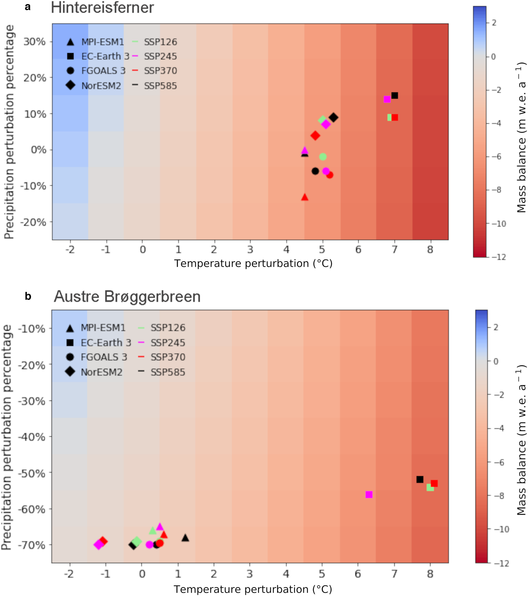
Figure 6. Response surfaces for Austre Brøggerbreen (a) and Hintereisferner (b), with the SSPs for all models overlaid, averaged over the period 2010–2040. Note the difference in precipitation axes for the two glaciers.
5. Discussion
The methods applied here depart from the conventionally used top–down approach of modeling glacier response to pre–defined climate change scenarios. We discuss the results in the context of the aims laid out in the introduction.
5.1 Case study application
The first aim is to apply a scenario–neutral approach to four glaciers as a case study, introducing an easy way to study glacier sensitivity, applicable worldwide. The global application is possible because of the availability of pre–processed directories, calibrated glacier–by–glacier. This approach is very simple and does not provide a perfect match between observed/real–world and simulated mass balance for every time period. This is evident from the mean error of 0.63 m w.e. a−1 for the Abramov Glacier (2), when simulating the period 1985–2015, whereas the mean error is 0 m w.e. a−1 when simulating the reference period 2000–2019. This large possible error and the limitation of static mass balance modeling provide the largest uncertainties in the application of this method. The main benefits of this method are the ease of generation and the global scale. The ability to generate a response surface for every glacier worldwide gives the opportunity to quickly gauge and compare glacier sensitivity for multiple glaciers. Comparing response surfaces at equal climate perturbations makes it possible to rapidly gauge differences between glaciers or at what perturbation X a certain threshold Y would be exceeded. This can also be implemented dynamically, with annual perturbations of temperature and precipitation, modeling glacier area or volume relative to an initial state. Doing this simple analysis for many glacier simultaneously and plotting results together can give a broad, organized overview of glacier response to changes in climate, even in data–sparse regions.
Especially for regions such as New Zealand, where glacier sensitivity has not been widely researched, yet glaciers are highly sensitive (Anderson and others, Reference Anderson2010), this is an advantage for the early stages of study design and can benefit communication with stakeholders. Even though the amount of water stored in New Zealand glaciers only represents 0.15 mm of sea level equivalent, the glaciers are important for hydroelectric power generation in the region (Anderson and others, Reference Anderson2010). The easily interpretable response surfaces clearly convey the impact of climate change to interested decision–makers. Being able to tailor the response surfaces to specific boundaries and local glaciers adds local context, unavailable from many top–down studies (Conway and others, Reference Conway2019).
5.2 Integration with a top–down approach
The second aim is to show the integration with a top–down approach. This is done in the simple but common manner of superimposing future climate change scenarios onto the response surfaces. The main goal of this particular top–down and bottom–up integration is to gauge the differences between projections and models and have a first translation of perturbations into responses. The differences between the four models and scenarios point to a high potential uncertainty in the use of climate change projections. The first translation of uncertainties from climate variables to mass balances adds information that a pure local climate comparison would not. The information gained through this integration feeds information back for a top–down approach: it can aid in model and scenario selection for multi–model ensembles or intercomparison studies. On shorter time scales, such as the decadal scale, fixed geometry mass balance still matches observed balances well (van der Laan and others, Reference van der Laan, Vlug, Scaife, Maussion and Förster2024). In these instances, superimposing scenarios on a response surface can provide a useful first step for dynamical modeling studies, as they can be done before running the computationally expensive impact model. This type of rapid assessment is generally considered the greatest asset of scenario-neutral approaches in climate change studies (Prudhomme and others, Reference Prudhomme, Wilby, Crooks, Kay and Reynard2010; Kay and others, Reference Kay, Crooks and Reynard2014).
Besides feeding back information for top–down approaches, the integration here emphasizes the local characteristics of bottom–up methods. Top–down methods would typically look at a multi–model ensemble mean of results and a larger scale, in terms of system response. In this integration however, the bottom–up characteristics of local response (one glacier) and vulnerability and risk (very negative mass balance at EC-Earth SSPs) are emphasized (Girard and others, Reference Girard, Pulido-Velazquez, Rinaudo, Pagé and Caballero2015). Integrated approaches, even as rudimentary as this one, are an example of how GCMs can inform analysis before being used as model forcing (Brown and Wilby, Reference Brown and Wilby2012).
5.3 Benefits to decision–making and communication
The third aim is to outline how this method could benefit decision–making and communication needs regarding glacier response to climate change. For decision–making, its strengths are in the local focus and the method potentially precluding an expensive, top–down climate impact assessment for a decision–maker's risk analysis (Brown and Wilby, Reference Brown and Wilby2012). Particularly on the short to medium term, climate assessments are relevant to decision–making (Patro and others, Reference Patro, De Michele and Avanzi2018). From our method, especially the seasonal sensitivity component can be useful. By keeping one season unperturbed, the impact of perturbations in the other can be isolated. When keeping perturbation ranges the same, comparisons of responses can be made between glaciers, as is done here for Hintereisferner and Austre Brøggerbreen. This provides insight into the differing importance of single seasons and climate characteristics per glacier. Many mass balance studies, including for some WGMS reference glaciers, only explore annual mass balance and continuous mass balance observations are only available for very few glaciers (Landmann and others, Reference Landmann2021). This limits our ability to determine the sensitivity of glaciers to temperature or precipitation directly. Response surfaces can provide insight into the effects of specific climate variables here, by showing different combinations of perturbed variables along the axes.
A use case example would be water availability for hydropower in the Alps, using seasonal sensitivity analysis. Glacier retreat is the major driver in the reduction of hydropower production in the Italian Alps, making climate change a large risk in decision–making processes in this industry (Patro and others, Reference Patro, De Michele and Avanzi2018). The current method can be useful in modeling mass balance for the upcoming season. OGGM would be forced with the known values for the preceding season, an average of previous values for the season to be modeled, and plausible perturbations. This gives a range of outcomes for the upcoming season, independent of scenarios, which is especially important when the preceding season was out of the ordinary. An example is the winter 2022–2023, which was strongly below the 2012–2022 accumulation average for Swiss glaciers (Switzerland, Reference Switzerland2022). Seasonal modeling of glaciers with a simple temperature index model, especially for the upcoming season, is difficult because of limited immediate availability of short–term re–analysis or model products of temperature and precipitation. Additionally, it is challenging to predict temperature and precipitation at high elevation and in complex topography (Goger and others, Reference Goger, Rotach, Gohm, Stiperski and Fuhrer2016), where glaciers are often located. The current scenario–neutral method can provide an approximation of the upcoming season, resulting in a response surface with the likely boundaries of annual balance after such a dry winter. The results of such a study are especially interesting, but difficult to obtain using top–down methods, on the short–term, to e.g. assess risk of low production for hydropower stakeholders. Overall, for decision–making processes with short lead times, such as hydropower or the planning of artificial snow capacity on glaciers in the ski industry, such rapid and simple forecasts can provide important insights (Doyle, Reference Doyle2014).
As a communication tool, response surfaces provide an intuitive way of understanding glacier responses. In hydrological modeling, they are recognized as a flexible, visual tool to promote understanding (Hirpa and others, Reference Hirpa, Dyer, Hope, Olago and Dadson2018). A quantification of glacier sensitivity can be difficult to grasp, especially for a non-specialist. Visual response surfaces for glaciers with different sensitivities make clear how identical perturbations in climate can have non–identical impacts. Climate change is also often perceived as an abstract problem, creating psychological distance between the public and the issue (Weber, Reference Weber2010; Pahl and others, Reference Pahl, Sheppard, Boomsma and Groves2014). A participant or stakeholder is more likely to be moved by climate change impact on a location (glacier) they have visited or live close to (Pahl and others, Reference Pahl, Sheppard, Boomsma and Groves2014). This psycho–social effect can heighten urgency and engagement (Luís and others, Reference Luís2018). The possibility of using this method rapidly, for any glacier in the world, can foster connection with the public through local knowledge. Because of the modular and open–source nature of OGGM, which includes an extensive educational platform (OGGM Edu, OGGM, 2022), the response surface function can be added to the list of model functions and can be included in an easily accessible OGGM (Edu) tutorial. This allows students to generate response surfaces for any glacier they are interested in. Through the response surfaces, glacier sensitivity to climate change can be illustrated, in addition to OGGM Edu applications such as the mass balance simulator. The method can easily be extended from the four glaciers presented here to all glaciers listed in the RGI. This type of visualization of climate science, understandable but backed–up by data and methods, is important for community engagement and learning (Sheppard and others, Reference Sheppard2011). The scenario–neutral approach can contribute to this.
5.4 Limitations and outlook
Finally, while scenario-neutral approaches can be useful, there are important limitations to the interpretation of the method presented here. The most limiting factor for both the glacier sensitivity index GSI T and response surfaces is the difference between fixed geometry mass balance and dynamical mass balance. Especially on longer time scales, mass balances develop with both the climate and the glacier's changes in area, volume and altitude. That is why the response surfaces here cannot be interpreted as the true glacier response to climate change and are mainly useful on shorter time scales.
We also conclude that the GSI T is a largely unnecessary complication of the method. Excellent work in the quantification of glacier sensitivity has been done by e.g. Oerlemans and Fortuin (Reference Oerlemans and Fortuin1992), Fischer (Reference Fischer2010) and more recently Krampe and others (Reference Krampe, Arndt and Schneider2022). While we have confirmed that calculating the glacier sensitivity index GSI T works, the utility of the scenario–neutral approach does not lie in the GSI T but rather in the visual response surfaces. The choice to not omit the glacier sensitivity index stems solely from its use in comparing results for our case study glaciers to previous literature.
Future applications of scenario–neutral mass balance modeling would mainly benefit from the method's simplicity. This is especially beneficial in three use cases: as an exploratory step when comparing glaciers, sensitivities or fixed scenarios, as an estimation of the upcoming mass balance season and as an educational tool. For the first case, it is beneficial that this approach is simple to implement on a global scale.
6. Conclusion
Overall, scenario–neutral methods can provide a useful, complementary approach to traditional top–down methods. The results for the four case study glaciers suggest the applicability of the method to individual glaciers on a global scale. The main added value of this method lies in its simple application, suitable for use cases like rapid sensitivity comparisons for a multitude of glaciers or the initial design of a study of a data–sparse region. An example of integrating top–down and bottom–up approaches is the overlaying of scenario projections onto response surfaces. This can deliver a first analysis, in which the response surface becomes the framework for comparing models and scenarios. It provides an initial translation of changing climate attributes into responses. For decision–making processes, the method's strengths lie in seasonal approximation, which is difficult to obtain quickly and for the right location using traditional approaches. Especially after a season with uncommon temperatures or precipitation, the scenario–neutral method can provide a first insight into the range of responses for the full year. The ability to apply the approach to a specific, local glacier can have a positive effect on decision–makers’ and public engagement. Finally, because of its intuitive visual output, the method presented here can be an important tool for science communication, for example in the Edu section of OGGM. Its simplicity comprises a limitation as well as a benefit. Overall, the scenario–neutral approach in OGGM can provide a complementary and useful approach to glacier mass balance modeling.
Acknowledgements
We would like to thank Lizz Ultee for her advice, motivating words and helpful discussions regarding this project. Thanks also goes out to Fabien Maussion, for building the OGGM community and his constructive comments that helped this research underway. This project was funded by the German Research Foundation, Project GLISSADE, no. 416069075


 Open access