


1. Introduction
Recent interests in unmanned underwater vehicles and micro air vehicles have motivated the desire to emulate the characteristic performance of animals’ swimming and flying. In nature, animals vary significantly in body size and moving speed, from small creatures (zebrafish larvae, tadpoles), to medium creatures (stingrays, reptiles and marine birds) and large mammals (manatees, dolphins, belugas and blue whales). As a result, the Reynolds number of natural swimming and flying spans nearly eight orders of magnitude (Gazzola, Argentina & Mahadevan Reference Gazzola, Argentina and Mahadevan2014). The critical Reynolds number was estimated to be approximately 3000, which is a crossover from the laminar to turbulent regimes. Among the various species, larvae and a small portion of amphibians live in the laminar regime, whereas most animals live in the turbulent regime.
Several review papers (Triantafyllou, Triantafyllou & Yue Reference Triantafyllou, Triantafyllou and Yue2000; Lauder Reference Lauder2015; Smits Reference Smits2019; Zhang, Zhang & Huang Reference Zhang, Zhang and Huang2022b) have introduced comprehensively the recent progresses in the hydrodynamics of aquatic locomotion and aerodynamics of airborne flight. Although study on the flow around real living animals is the most direct approach for understanding biological kinematics and fluid dynamics, the research object is limited to relatively small-size species with low and intermediate  $Re$, such as eels (Tytell Reference Tytell2004; Tytell & Lauder Reference Tytell and Lauder2004), zebrafish (Guo et al. Reference Guo, Kuai, Han, Xu, Fan and Yu2022), sunfish (Drucker & Lauder Reference Drucker and Lauder2000), dragonflies (Thomas et al. Reference Thomas, Taylor, Srygley, Nudds and Bomphrey2004) and hummingbirds (Pournazeri et al. Reference Pournazeri, Segre, Princevac and Altshuler2013). Moreover, force measurement and high-quality three-dimensional (3-D) flow visualization for a living body is a challenging task, which is important to reveal the flow physics of swimming and flying. Experimental study using robotic or simplified model and numerical work largely enriched the object, e.g. tuna (Zhu et al. Reference Zhu, Wolfgang, Yue and Triantafyllou2002; Zhong, Dong & Quinn Reference Zhong, Dong and Quinn2019; Zhong et al. Reference Zhong, Zhu, Fish, Kerr, Downs, Bart-Smith and Quinn2021), manta, bat (Wang et al. Reference Wang, Zhang, He and Liu2015a). Besides, numerical work gave us more detailed flow information. However, studying the swimming and flying problems at high Reynolds numbers remains a challenge (Dong et al. Reference Dong, Bozkurttas, Mittal, Madden and Lauder2010; Borazjani & Daghooghi Reference Borazjani and Daghooghi2013; Fish et al. Reference Fish, Schreiber, Moored, Liu, Dong and Bart-Smith2016).
Zhang et al. (Reference Zhang, Zhang and Huang2022b) summarized the Reynolds numbers employed in approximately 60 studies of aquatic animals (figure 1) and showed that experiments generally were conducted under higher- $Re$ conditions than numerical studies. The Reynolds numbers of most high-fidelity numerical simulations were below
  $10^4$, due to the high requirement of a fine grid for resolving the boundary layer near the body and the wake flow. Among the numerical work shown in figure 1, the highest
  $Re$ was considered by Bottom et al. (Reference Bottom II, Borazjani, Blevins and Lauder2016), who simulated the swimming stingrays at
  $Re=13\,500$ and 23 000. They showed the existence of a leading-edge vortex (LEV) on stingrays and the LEV was related to the thrust and efficiency enhancement. But the authors did not discuss the effect of Reynolds number and the LEVs remained coherent structures in this
  $Re$ range. Oh et al. (Reference Oh, Lee, Park, Choi and Kim2020) conducted a numerical study on the aerodynamic performance of a hovering rhinoceros beetle at
  $Re=12\,000$, in which a great deal of small-scale vortices were visible. However, their work focused on developing a predictive quasisteady theory, whereas the dynamics of vortical structures was not further investigated. Besides, Khosronejad et al. (Reference Khosronejad, Mendelson, Techet, Kang, Angelidis and Sotiropoulos2020) performed large-eddy simulation (LES) of an archer fish jumping from water into air at
  $Re$ of 60 000. The findings for the stages in water agree with the traditional reverse Kármán vortex street. Daghooghi & Borazjani (Reference Daghooghi and Borazjani2015) conducted simulations of mackerels swimming in a rectangular pattern at
  $Re$ of 50 000. The present work improves the Reynolds number of high-fidelity numerical simulations to
  $O(10^5)$.

Figure 1. Reynolds numbers used in recent studies, where a circle represents high-fidelity numerical work (labelled by  $N$) and a cross represents experimental work (labelled by
  $E$). Adapted with permission from Zhang et al. (Reference Zhang, Zhang and Huang2022b).
In fact, the effect of Reynolds number has been reported in previous studies. Bozkurttas et al. (Reference Bozkurttas, Mittal, Dong, Lauder and Madden2009) examined the performances of a deformable fish pectoral fin at  $Re=540, 1440, 6300$. The forces reduced with decreased
  $Re$, but they had similar variation trends. The forces were reduced to as high as
  $40\,\%$. Regarding the vortical structures, small-scale vortices were dissipated but the key features of vortices were similar. Borazjani & Sotiropoulos (Reference Borazjani and Sotiropoulos2008, Reference Borazjani and Sotiropoulos2009, Reference Borazjani and Sotiropoulos2010) conducted a series of simulations at
  $Re=300, 4000$ (viscous flow) and
  $\infty$ (inviscid flow) to investigate the performances of carangiform and anguilliform locomotion. The critical Strouhal number, at which the self-propelled state is reached, is decreased with the increasing
  $Re$ for both swimmers. The propulsive efficiency of the carangiform swimmer is an increasing function of
  $Re$, while the effect of
  $Re$ on the efficiency of the anguilliform swimmer is different. Shyy & Liu (Reference Shyy and Liu2007) presented the effect of Reynolds number on vortex stability by comparing the vortical structures of flying insects at
  $Re=10, 100, 6000$. The conical LEV was observed to break down at
  $Re=6000$, whereas it attached stably on the wing and connected to the tip vortex (TV). Kim & Gharib (Reference Kim and Gharib2010) found that the starting vortex cannot be formed in the wake of a rotating plate at
  $Re = 60$ as distinctly as that at
  $Re = 8800$. Harbig, Sheridan & Thompson (Reference Harbig, Sheridan and Thompson2013) simulated a fruit fly wing at
  $Re = 120\unicode{x2013}1500$. Increasing
  $Re$ led to the development of a dual LEV structure, and the increase of the aspect ratio had similar effect. It was also observed that some major mechanisms employed by animals were kept the same for different Reynolds numbers, such as those of body–fin interaction (Liu et al. Reference Liu, Ren, Dong, Akanyeti, Liao and Lauder2017) and fin–fin interaction (Zhang, Sung & Huang Reference Zhang, Sung and Huang2020). Han, Chang & Kim (Reference Han, Chang and Kim2014) experimentally investigated the dependence of an insect flapping wing on the Reynolds number. At
  $Re = 7200$, the lift was enhanced due to the wing–wake interaction and the pitching-up rotational mechanism, whereas at
  $Re = 23\,000$, the lift peak standing due to the wing–wake interaction was delayed, and the lift augmentations due to pitching-up rotation disappeared. From their digital particle image velocimetry results, the LEV in the rotational phase cannot maintain its attachment and the trailing edge vortex (TEV) is underdeveloped. Moreover, the flow field exhibits some turbulent characteristics.
As seen above, low to moderate  $Re$ condition was widely adopted in the previous numerical studies, whereas high-fidelity 3-D simulations at high
  $Re$ of aquatic animals are rare. The effect of Reynolds number has not been well understood yet, especially at the high-
 $Re$ range. In the present study, the batoid fish is chosen as a typical aquatic species because it has large propulsion area compared with the species using body/caudal fins, around which the flow is easier to be fully developed and the effect of Reynolds number is more notable. The simulations are performed at the Reynolds number of up to 148 000, while those at lower
  $Re$ (i.e.
  $Re=1480, 14\,800$) are also performed in order to reveal the effect of Reynolds number varied across three orders of magnitude. The present study aims to answer the following questions. (1) What are the main features of the flow field of a swimming batoid fish at the real swimming Reynolds number and their effects on the performance? (2) What is the effect of Reynolds number in a relatively wide
  $Re$ range across the laminar and turbulent regimes? (3) Can the results under the widely adopted low to moderate
  $Re$ condition represent those at high
  $Re$?
$Re$?
The rest part of the work is structured as follows. The physical model and numerical method are introduced in § 2, the results are presented in § 3, including the hydrodynamic forces, the mean flow and fluctuating characteristics and the vortex dynamics. Then, further discussion is given in § 4, and finally in § 5 conclusions are drawn, which (partially) answer the above questions.
2. Physical model and numerical method
Figure 2 displays a 3-D morphological model of the batoid fish (cownose ray, Rhinoptera javanica) which was constructed based on several section profiles (Huang, Zhang & Pan Reference Huang, Zhang and Pan2020). The model has a dorsoventrally flattened body with a length of  $BL$ and expanded pectoral fins with a span of
  $SL$. The kinematics model was constructed based on the data from high-resolution digital camera recordings of free-swimming batoid fish specimens by tracking some characteristic points, such as the head, tail base and pectoral fin tip. Batoid fish is a good example that actively controls its fin shape, and a prescribed kinematic equation can be employed to describe its deformation. The main deformation can be decomposed into the spanwise and chordwise components, which are described by using a rotational motion around the longitudinal (
 $x$) axis of the body associated with spanwise flexibility and a chordwise travelling wave, respectively. The wavenumber for a cownose ray was chosen as 0.4. In our simulations, the tethered model was adopted, i.e. the batoid fish swims against a constant inflow without moving in the
  $x$-direction. The motion of the body is prescribed as the kinematic model, in which the deformation at the plane of
  $y/SL=0$ is zero. Details of the mathematical description can be found in our previous work (Zhang et al. Reference Zhang, Huang, Pan, Yang and Huang2022a).

Figure 2. (a) The living cownose ray and (b) our constructed cownose ray model.
The immersed boundary (IB) method has been widely used in numerical studies of flying and swimming at low- to moderate- $Re$ conditions (Peskin Reference Peskin2002; Zhu et al. Reference Zhu, He, Wang, Miller, Zhang, You and Fang2011; Sotiropoulos & Yang Reference Sotiropoulos and Yang2014). In order to simulate the flow over the batoid fish at relatively high Reynolds numbers, the wall-modelled large-eddy simulation (WMLES) in conjunction with the IB method is employed (Ma, Huang & Xu Reference Ma, Huang and Xu2019). The governing equations are the filtered incompressible Navier–Stokes equations,
 \begin{equation} \left.\begin{gathered} \frac{\partial \tilde{u}_i}{\partial t} +\frac{\partial \tilde{u}_i \tilde{u}_j}{\partial x_j} = \frac{\partial \tilde{p}}{\partial x_i}- \frac{\partial \tilde{\tau}_{ij}}{\partial x_j} + \frac{1}{Re} \frac{\partial \tilde{u}_i}{\partial x_j \partial x_j} +f_i, \\ \frac{\partial \tilde{u}_i}{\partial x_i} =0, \end{gathered}\right\} \end{equation}
where  $\tilde {u}_i$ is the filtered velocity,
  $\tilde {p}$ denotes the filtered pressure,
  $f$ denotes the additional momentum force obtained by the penalty IB method (Huang, Chang & Sung Reference Huang, Chang and Sung2011). The Smagorinsky subgrid model is adopted to compute the subgrid scale stresses. The wall model is implemented by solving the thin boundary layer equation on an embedded mesh refined along the wall-normal direction. Then, the wall shear stress is inserted into the LES solution through a dynamic matching procedure. The second-order central finite difference scheme is used to discretize the equations, and time is advanced by a fully implicit Crank–Nicholson scheme. Moreover, the velocity pressure is decoupled by using the fractional step method. The present numerical solver has been validated through various tests, such as turbulent flows over periodic hills (
 $Re=1.1\times 10^5$), over a travelling wavy wall (
 $Re=1.0\times 10^5$), in circular pipe (
 $Re=1.4\times 10^5$) and over a pitching airfoil (
 $Re=4.8\times 10^4$) in our previous studies (Ma et al. Reference Ma, Huang and Xu2019, Reference Ma, Huang, Xu and Cui2021). These tests were within the
  $Re$ range considered in the present work and showed that the proposed IB-WMLES method is a reliable tool to deal with the high-
 $Re$ flow problems.
In the present simulations, the Cartesian mesh was adopted. The computational domain size was chosen as  $5.4BL \times 2.7BL \times 2.7BL$ and
  $2501 \times 371 \times 1251$ grid points. Near the body, a uniform grid with the resolution of
  $0.002BL$ was adopted, corresponding to the largest
  $y^+$ of 32 with the superscript ‘
 $+$’ denoting normalization by the wall viscous unit. In the IB method, since the Cartesian grid was used instead of body-fitted mesh, the distance from the first grid to the body surface is varied around the body. Notably, the distance is within one Eulerian grid size, and thus we used
  $0.002BL$ to compute
  $y^+$. Away from the body, stretched grids were employed in the normal (
 $z$) direction, whereas uniform grids were still used in the streamwise (
 $x$) and spanwise (
 $y$) directions. The time step was set as
  $T/8000$, where
  $T$ is the stroke period, and the corresponding Courant–Friedrichs–Lewy number is approximately 0.3. Such parameters are based on the extensive domain- and grid-independence study. In the domain-independence study, a larger domain (
 $8.1BL \times 2.7BL \times 4.1BL$) was tested and the results showed little difference in the force coefficients. For the grid-independence study, a coarse grid case with
  $2001 \times 351 \times 1001$ grid points as well as a fine grid case with
  $3125 \times 391 \times 1563$ grid points was conducted. Figure 3 shows a comparison of the thrust coefficient and power coefficient for the three grid cases at
  $Re=148\,000$. It shows that the maximum differences in the thrust and power coefficients are 2.6 % and 1.7 %, between the fine and medium grid cases, respectively. The simulations were performed on a supercomputing cluster using 64 AMD 2.35 GHz processors.

Figure 3. Grid-independence study at  $Re=148\,000$ on the (a) thrust coefficient
  $(C_T)$ and (b) power coefficient
  $(C_{PW})$ with three different grids, i.e. the coarse grid (
 $2001 \times 351 \times 1001$), the medium grid (
 $2501 \times 371 \times 1251$) and the fine grid (
 $3125 \times 391 \times 1563$).
3. Results
In the present study, simulations of the swimming batoid fish at three Reynolds numbers ( $Re=1480$, 14 800 and 148 000) were carried out. The Reynolds number is defined as,
  $Re=U_\infty BL/\nu$, where
  $U_\infty$ is the inflow velocity and
  $\nu$ is the kinematic viscosity. The tip-to-tip amplitude (
 $A$) is
  $0.6BL$ and the frequency (
 $f$) is 0.7 Hz, resulting in a Strouhal number (
 $St=fA/U_\infty$) of 0.39. In each case, seven stroke cycles were simulated. In § 3.1, the instantaneous forces were obtained from the seventh stroke cycle. After approximately one stroke cycle, the flow reaches the periodic state. Thus, in § 3.2, the mean flow field was calculated using the data of the latest six stroke cycles.
3.1. Hydrodynamic performance
Table 1 shows the cycle-averaged forces at the three Reynolds numbers and figure 4 shows the variation of the forces on the model. In order to examine how the increase in the Reynolds number affects the net thrust ( $T$), we further focus here on the pressure (
 $FP$) and viscous (
 $Ff$) components of the thrust. All forces are non-dimensionaliszed by
  $0.5\rho U_\infty ^2 BL^2$, where
  $\rho$ is the density of the fluid. In addition, the power consumed to propel the batoid fish is also computed by integrating each boundary element's power due to the deformation velocity
  $\boldsymbol {U_{body}}$, i.e.
 \begin{equation} PW=\int_\varOmega \boldsymbol{F_L} \boldsymbol{\cdot} \boldsymbol{U_{body}} \,{\rm d} s , \end{equation}
where  $\boldsymbol {F_L}$ is the Lagrangian force at each boundary element
  $ds$. Here
  $PW$ is normalized by
  $0.5\rho U_\infty ^2 BL^3$,
  $\boldsymbol {U_{body}}$ is computed using the equation of body motion (Zhang et al. Reference Zhang, Huang, Pan, Yang and Huang2022a) at two instants
  $\boldsymbol {U_{body}}=(\boldsymbol {x}(t2)-\boldsymbol {x}(t1))/(t2-t1)$. Here the quasipropulsive efficiency
  $\eta _{QP}$ (Maertens, Triantafyllou & Yue Reference Maertens, Triantafyllou and Yue2015) is adopted to measure the swimming efficiency, which is defined as
 \begin{equation} \eta_{QP}=\frac{(\bar{T}+\bar{R})U_\infty}{\overline{PW}}, \end{equation}
where  $\bar {T}$ is the averaged thrust obtained by integration of
  $-\boldsymbol {F_L}$ over body surface and time, and
  $\bar {R}$ is the towed resistance with a steady stroking position over a cycle (
 $t/T=0.17$) with zero velocity on the surface at a speed
  $U_\infty$ and an overbar is used to indicate a time-averaged value. Here we choose the midstroke
  $t/T = 0.17$ because the motion at upstroke is asymmetrical to that at downstroke. As shown in table 1, the thrust increases as the
  $Re$ increases. It is only at
  $Re=148\,000$ that the model generates a positive thrust. Since the tethered model is used in our simulations, a negative thrust means that with the present inflow condition and kinematics, the fish cannot keep equilibrium in a free-swimming state and has to work harder to achieve the given velocity in the still water. Such a result can be understood from the pressure and friction forces, i.e. the positive thrust comes from the increase of the pressure force and decrease of the friction drag. As
  $Re$ increases by two orders of magnitude,
  $\bar {C}_{Ff}$ decreases by an order of magnitude. Difference in
  $\bar {C}_{FP}$ is due to the vortex dynamics, which causes the pressure distribution to vary and will be presented in the following sections. The swimmers consume more energy as
  $Re$ increases, while the efficiency is also improved. Here, the traditional net efficiency
  $\bar {T}U/\overline {PW}$ was not employed because the net thrust at
  $Re=1480$ and 14 800 is negative. Note that the efficiency is not strictly less than one because the drag at the towed state is larger than that at the swimming state. Similar phenomena can also be seen in the previous studies (Maertens et al. Reference Maertens, Triantafyllou and Yue2015; Zhang et al. Reference Zhang, Zhang and Huang2022b). The instantaneous forces are shown in figure 4. It is found that there is relatively little change in the tendency of temporal variation of the forces. The forces peak at the midstroke and reach the valley at the start/end of the stroke. Notably, the second peak of the force coefficients at the midupstroke is not equal to the first one. At
  $Re=148\,000$, such a difference is more significant. The reason is that the flow is downstroke–upstroke asymmetrical due to the asymmetrical shape of batoid fish. A higher Reynolds number leads to a more distinct asymmetrical flow, causing a more obvious difference in the force peaks.
Table 1. Cycle-averaged force coefficients at different  $Re$.
$Re$.


Figure 4. Comparisons of instantaneous (a) thrust  $(C_T)$, (b) pressure force
  $(C_{FP})$, (c) friction force
  $(C_{Ff})$ and (d) power
  $(C_{PW})$ coefficients for a batoid fish swimming at
  $Re = 1480$, 14 800 and 148 000.
3.2. Mean flow topology
Figure 5 displays the contours of time-averaged streamwise velocity at the plane of  $z/BL=0$ at
  $Re=1480, 14\,800$ and 148 000, where the velocity is normalized by the inlet velocity
  $U_\infty$. To demonstrate the effects of Reynolds number on the mean flow topology, we focus on two regions, i.e. the recirculation zone and the tip region. At
  $Re=1480$, there is a long recirculation zone behind the batoid fish. As shown in figure 5(a), the isocontour of 0.05 is extended to position
  $x/BL=1.35$; whereas in figures 5(b) and 5(c), the recirculation zone is significantly shortened. The pressure drag is closely related to the flow separation at the recirculation zone. Such a difference implies a smaller body drag at higher Reynolds number. At the tip region, a jet flow is visible in figures 5(b) and 5(c). The jet flow with an increased streamwise velocity compared with the inflow coincides with the result of a manta ray (Fish et al. Reference Fish, Schreiber, Moored, Liu, Dong and Bart-Smith2016), which accounts for the thrust force generated at the tip region. As the Reynolds number increases, it generates a longer jet flow, indicating a lager thrust. At
  $Re=1480$, no obvious jet flow is detected, resulting in a drag-like wake.

Figure 5. Contours of time-averaged streamwise velocity at (a)  $Re=1480$, (b)
  $Re=14\,800$ and (c)
  $Re=148\,000$ at the plane of
  $z/BL=0$, where
  $U_\infty$ is the inlet velocity.
To demonstrate the mean wake flow more clearly, the mean velocity profiles at different streamwise positions are shown in figure 6, where the positions are labelled in figure 5(c). Due to the high cost of long-time simulation, only six stroke periods were employed for averaging. In order to obtain a smooth profile, the velocities are further averaged along the streamwise direction, from plane A to B ( $x/BL=0.97-1.24$), B to C (
 $x/BL=1.24-1.51$) and C to D (
 $x/BL=1.51-1.78$). Actually, from figure 6(a), the lowest Reynolds number generates a slight jet flow, which does not exceed 1.05
 $U_\infty$. However, the jet flow region is very limited, at
  $\vert y/SL \vert > 0.66$. In contrast, the magnitude of the jet flow at the other two Reynolds numbers can be as high as 1.1
 $U_\infty$ with an extended region reaching
  $\vert y/SL \vert = 0.50$. The difference of jet flow length between
  $Re=14\,800$ and 148 000 (figures 5b and 5c) can be also found in the velocity profiles. In the C–D region (figure 6c), which is far away from the model, the maximum jet velocity is 1.05
 $U_\infty$ at
  $Re=14\,800$; whereas it exceeds 1.07
 $U_\infty$ at
  $Re=148\,000$, reflecting a stronger jet flow. For the recirculation zone, it takes longer for the flow at lower Reynolds numbers to recover to the inflow velocity. For example, as shown in figure 6(b), the velocity at
  $y/SL=0$ is nearly zero at
  $Re=1480$, whereas an increased velocity can be observed at higher Reynolds numbers. At the region farther away from the body, the flows at
  $Re=14\,800$ and 148 000 have almost the same profile.

Figure 6. Time- and streamwise-averaged velocity profile between different Reynolds numbers. Here, the data is averaged by six stroke periods and positions taken at slice cuts from (a) A to B ( $x/BL=0.97-1.24$), (b) B to C (
 $x/BL=1.24-1.51$) and (c) C to D (
 $x/BL=1.51-1.78$), which are labelled in figure 5.
Figure 7 presents the time-averaged streamwise velocity at the  $y/SL=0$ plane. As expected, higher-
 $Re$ flow has a thinner boundary, suggesting a fuller velocity profile. From the surface friction distribution as shown in figure 8, a high-friction region is observed, which is reduced significantly as the Reynolds number increases. At the highest Reynolds number (figure 8c), the high-friction region is concentrated only near the leading edge, whereas at
  $Re=1480$, the high-friction region occupies almost the whole surface (figure 8a). Moreover, in figure 7, a negative velocity displayed by grey colour is added to demarcate the reversed flow region. The reversed flow in the wake is consistent with the recirculation zone as seen in figures 5 and 6.

Figure 7. Time-averaged streamwise velocity at (a)  $Re=1480$, (b)
  $Re=14\,800$ and (c)
  $Re=148\,000$ at the plane of
  $y/SL=0$. The grey region represents the boundary of reverse flow (negative
  $u$).
$u$).

Figure 8. Time-averaged (a–c) frictional coefficient  $(C_f)$ and (d–f) pressure coefficient
  $(C_p)$ distribution on the model surface at (a,d)
  $Re=1480$, (b,e)
  $Re=14\,800$ and (c, f)
  $Re=148\,000$. Here
  $C_p=(p-p_\infty)/(0.5 \rho U_\infty^2)$.
The reversed flow region at the suction surface of the model in the time-average sense is commonly referred to as a laminar separation bubble (LSB) (Tani Reference Tani1964). A typical structure of a two-dimensional (2-D) mean LSB occurs between the separation and reattachment locations (Horton Reference Horton1968). The separation originates from a laminar boundary layer subjected to an adverse pressure gradient, whereas the reattachment is usually due to the laminar shear layer transition to turbulence. At the  $y/SL=0$ plane, LSB occurs only at the posterior, connecting the wake recirculation zone at
  $Re=1480$. Long LSB occurs at
  $Re=14\,800$. Notably, behind the reattachment point, another separation point was also observed, which is different from the typical LSB structure. This is analysed using the instantaneous flow in the following section. At the highest Reynolds number, there is no obvious reversed flow region, indicating a smaller drag force. From the time-averaged pressure distribution (figure 8d–f), at the leading edge of the body, a low-pressure region is formed, which is created due to the LEV. As
  $Re$ increases, the magnitude of the low-pressure region increases. It can be seen that the pressure at the posterior region is higher than that at the front, thus creating a pressure difference, i.e. the thrust force. The lower pressure at the leading edge accounts for the larger thrust force at higher
  $Re$ as seen in table 1.
3.3. Vortical structures
3.3.1. Overview of the vortical structures
Vortex evolution is known to play a key role in the hydro/aerodynamics of swimming and flying (Liu, Du & Sun Reference Liu, Du and Sun2020; Zhang et al. Reference Zhang, Huang, Pan, Yang and Huang2022a). Figure 9 presents the time sequence of 3-D structures at the three Reynolds numbers during the downstroke, visualized by the isosurface of the  $Q$-criterion. The insets display the phase of the stroke motion and also the contours of the surface pressure coefficient. The flow can be divided into three regions: dorsal region, span region and tip region. At
  $Re=1480$, the LEV at the span region is stable, attaching to the surface due to strong viscous dissipation. A slender TV is formed and sheds off slightly at the tip region, whereas no structures are observed at the dorsal region. The attached LEV creates a low-pressure region. At mid-downstroke (figure 9b), the low-pressure reaches its peak and as the fins further stroke down (figure 9c), the low-pressure is reduced, indicating a weakened LEV. These results show good agreements with the previous numerical and experimental observations that the LEV does not shed off at low
  $Re$ (Lentink & Dickinson Reference Lentink and Dickinson2009; Chen et al. Reference Chen, Kolomenskiy, Nakata and Liu2017).

Figure 9. Comparisons of the 3-D wake structures of a batoid fish, between the models of (a–c)  $Re=1480$, (d–f)
  $Re=14\,800$ and (g–i)
  $Re=148\,000$, visualized by the isosurface of
  $Q = 80$, 300, 500, respectively, and coloured by streamwise velocity, at (a,d,g) the early downstroke (
 $t/T = 0.17$), (b,e,h) the mid-downstroke (
 $t/T = 0.33$) and (c, f,i) the late downstroke (
 $t/T = 0.50$).
At  $Re=14\,800$, the unsteadiness in the span and tip regions become noticeable, where the LEV breaks into several corotating vortical structures and a stronger spiral TV is shed into the wake (see figure 9d–f). A similar dual LEV system was observed over rotating insect wings for a range of wing shapes (Srygley & Thomas Reference Srygley and Thomas2002; Lu, Shen & Lai Reference Lu, Shen and Lai2006; Harbig et al. Reference Harbig, Sheridan and Thompson2013; Chen et al. Reference Chen, Kolomenskiy, Nakata and Liu2017). However, the LEV of the batoid fish splits into more structures and forms a multi-LEVs system. As the stroke goes on, the LEV convects downstream until the fins reverse their direction; then it is shed into the wake as a part of TEV during the upstroke. The multi-LEVs create long narrow low-pressure bands. Also visible is the moving of such low-pressure bands with the convection of LEV. Another distinctive feature is that the vortical structures are developed from the dorsal part of the batoid fish (dorsal vortex (DV)), and are shed into the wake at the end of downstroke (figure 9f). Actually, the formation of DV begins at the start of previous upstroke, when the LEV formed at previous downstroke just convects to the trailing edge (not show here). It is a result of the interaction between the dorsal shear layer and the convecting LEV formed during the previous stroke.
At  $Re=148\,000$, distinct differences can be observed in all the three regions. In the dorsal region, a large number of small-scale vortical structures are formed without coherent DV structures. The LEV splits into more LEVs in the span region (figure 9g), indicating it has a stronger instability. As the LEVs convect downstream, the vortex cores are more diffused (figure 9h). At the end of downstroke (figure 9i), small-scale vortical structures are likely to be dominant at the posterior of the batoid fish. In the tip region, the topology of TV is visible, however, with a diffused vortex core and a great deal of small-scale vortical structures. From the surface pressure contours, strong pressure fluctuation is found, which gives evidence of the existence of turbulent flow. The way these turbulent structures are formed and their effect on the pressure distribution are examined in detail in § 3.3.3.
3.3.2. Flow separation region
Pressure and skin friction distributions are commonly used to demonstrate the characteristics of LSB. There always exists a plateau downstream of the suction peak and then a rapid pressure recovery, representing the characteristics of flow separation and reattachment (Toppings & Yarusevych Reference Toppings and Yarusevych2021). Meanwhile, the skin friction vanishes at these locations. However, these may be more suitable to describe the separation location of 2-D flows (Délery Reference Délery2001). For 3-D flows, the skin friction lines, also known as the limiting streamlines, are a good way to describe the separation and reattachment (Délery Reference Délery2001). Another approach is the isosurface of zero streamwise velocity. Toppings & Yarusevych (Reference Toppings and Yarusevych2021) showed that the two approaches agree well in identifying the streamwise separation and reattachment bounds. The isosurface of zero streamwise velocity was used to show the streamwise and spanwise bounds of the flow separation region as shown in figure 10. It is observed that the separation location varies greatly with Reynolds number. At  $Re=1480$, separation takes place only near the trailing edge. This indicates there is a good flow attachment for most parts of the body. At
  $Re=14\,800$, the separation line moves upstream, starting at almost half of the body. Separated flow can be also seen near the centre line and the tip region. Substantial difference is found at
  $Re=148\,000$ with no obvious separation line. Moreover, the separation zone is discontinuous and scattered.

Figure 10. Isosurface of zero streamwise velocity at  $t/T=0.33$.
To describe the separation shape more clearly, the reversed flow region, visualized by  $u\leq 0$, was also displayed at the
  $x$–
$x$– $y$ plane
  $y/SL=0.62$ in figure 11. Actually, at the start of the downstroke (
 $t/T=0.17$) shown in figure 11(a), the flow does not separate near the surface at
  $Re=1480$. The result at
  $Re=14\,800$ shows the presence of a typical LSB without reattachment. As the viscous effect weakens at
  $Re=148\,000$, a similar LSB also occurs with the separation point moving upstream slightly. At the mid-downstroke (
 $t/T=0.33$), our previous study has already revealed that the effective angle of attack of the swimmer reaches its maximum at this moment (Zhang et al. Reference Zhang, Huang, Pan, Yang and Huang2022a). High effective angle of attack makes the flow easier to separate. Thus, at
  $Re=1480$, the reversed flow occurs at the trailing edge of the model, and at
  $Re=14\,800$, the reversed flow region extends farther upstream. Substantial difference is observed at
  $Re=148\,000$, where a long LSB transforms into many scattered reversed flow regions, indicating the occurrence of turbulent flow. The results are similar to the side view of the instantaneous flow downstream of the mean reattachment in the transition of flow over a flat plate (Alam & Sandham Reference Alam and Sandham2000). However, a distinction needs to be drawn that in the present simulation, no coherent LSB is observed upstream the turbulence region (Alam & Sandham Reference Alam and Sandham2000). This implies that the formation of the turbulent flow is different from the traditional one, which is described in § 3.3.3. At
  $t/T=0.5$, the reversed flow region continues to decrease with the turbulent structures convecting downstream. The separation positions are further quantitatively displayed in figure 12(a). Moreover, the length in one chord occupied by the reversed flow is also presented in figure 12(b). Results at
  $Re=1480,14\,800,148\,000$ are displayed by black, red and blue colours, respectively. Although a higher Reynolds number leads to the acceleration of the start of flow separation, the separate region is reduced apparently due to the transition to turbulence.

Figure 11. Streamwise velocity vectors and contours of flow separated region at slice-cut of  $y/SL=0.62$, (a)
  $t/T=0.17$, (b)
  $t/T=0.33$, (c)
  $t/T=0.5$.

Figure 12. (a) The separate position and (b) the length of the separate region at the slice-cuts of  $y/SL=0.62$ at
  $Re=1480$ (black), 14 800 (red), 148 000 (blue).
3.3.3. Formation of hairpin vortical structures
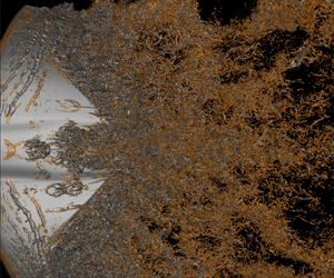
In § 3.3.1, a large number of small-scale vortical structures are formed at  $Re=148\,000$, among which the hairpin-like structures are visible by enlarging the figures (e.g. figure 13). The hairpin vortical (HV) structure is a basic flow structure of turbulent boundary layers (Adrian Reference Adrian2007). Some distinct types of hairpin vortex formation mechanism were observed in the present work. As discussed in § 3.3.1, three characteristic regions can be identified based on the vortical structures. In this section, the vortex formation processes in the three regions are described in detail.

Figure 13. Enlarged views at  $t/T=0.17$ to show the local vortical structures and spanwise vorticity contours at the selected planes A–A, B–B and C–C.
Figure 13 describes the local vortical structures at  $Re=148\,000$ in an enlarged view. At the dorsal region, two hairpin vortices packets can be clearly observed. These structures are developed from the upstream shear layer. The packet around the
  $y/SL=0$ position (labelled as A–A) contains three rows of hairpins. The younger hairpin (HV3) has a typical shape, i.e. one head aligned in the spanwise direction and two legs aligned in the streamwise direction, whereas the quasistreamwise legs of the older ones (HV1 and HV2) are more diffused. Notably, the hierarchy of multiscale vortices is observed, i.e. smaller-scale hairpin vortices (SVs) on the legs of the larger hairpin (HV3). These are qualitatively similar to those observed in a turbulent boundary layer at high Reynolds numbers (Motoori & Goto Reference Motoori and Goto2019), where the small-scale vortices are mainly stretched by the strain-rate field induced by large-scale ones. Interestingly, as convected downstream, the small-scale vortices can be further developed into new hairpins as their heads. Moreover, as the disturbance spreads laterally, HV3 produces similar configurations referred to as subsidiary vortices by Smith et al. (Reference Smith, Walker, Haidari and Sobrun1991), allowing the hairpin structures to spread in the spanwise direction. Another hairpin vortex packet around the plane B-B contains two individuals in line, where the legs of HV4 are developed beneath the head of HV5. Such a typical hairpin packet has been explored widely (Adrian Reference Adrian2007).
In the span region, it takes a longer period to form the hairpin-like structures, contrary to those in the dorsal region. The generation of hairpins in this region is related to the LEVs. From figure 13, it is shown that some corrugations identified as valleys and bulges are observed on the LEVs (e.g. LEV2). Such an observation is similar to that in the 3-D TEVs of an oscillating foil caused by elliptic instability in the wake (Verma & Hemmati Reference Verma and Hemmati2021). Meanwhile, the LEV2 begins to lift up away from the wall, coinciding with the flow separation described in § 3.3.2. In figure 14, we continue to depict the LEV to HV transformation from  $t/T=0.33$ to 0.67. As the pectoral fins stroke, the instability grows radially along the LEV. At
  $t/T=0.33$ (figure 14a), it leads to the exchange of flow between the LEVs and shear layer. Around the boundaries of the corrugations the flow curls into vortex filaments, referred to as the secondary filament (SF), perpendicular to the LEV tube. Once formed, the SFs convect downstream with the LEVs and they interact with each other. As the structures convect downstream, the SFs are continuously stretched by the vortex cores and the LEVs further split into smaller vortices, as shown in figure 14(b). Thus, the quasistreamwise SFs and spanwise broken LEVs form the so-called one-legged hairpin-like structures (Smith et al. Reference Smith, Walker, Haidari and Sobrun1991), as the legs and heads, respectively. Meanwhile, the SFs begin to form on the younger LEVs (LEV3, LEV4). When the fins reverse their directions (figure 14c), the structures finish their LEV to HV transformation.

Figure 14. The instantaneous local vortical structures at  $Re=148\,000$. The velocity legend is same as that in figure 13.
In the tip region, the pectoral fin has a higher flapping amplitude, resulting in a stronger instability. As observed in figure 14(a), the spanwise LEV7 soon loses its two-dimensionality with convection, generating a wavy shape. This shows that the disturbance starts to spread in the spanwise direction. The wavy LEVs then break into small-scale vortices, wherein the spanwise structures form the heads of hairpins (figure 14b). Simultaneously, the curved part of the structures is stretched progressively downward, forming the legs of hairpins. This process is similar to that on the surface of an airfoil (Sato et al. Reference Sato, Asada, Nonomura, Kawai and Fujii2017).
3.3.4. Effect of Reynolds number on vortex and pressure distribution
Figure 13 also compares the local structures through the  $Q$-isosurfaces and the spanwise vorticity contours at three selected planes at
  $Re=14\,800$ and 148 000. Vortices at
  $Re=1480$ are not displayed here because their simple topology has been clearly shown in figure 9. The spanwise vorticity has been known to have a thick boundary and is hard to separate at low Reynolds number simulations (Zhang et al. Reference Zhang, Pan, Chao and Zhang2018; Menzer et al. Reference Menzer, Gong, Fish and Dong2022). At
  $Re=14\,800$, the primary structures are large-scale structures, e.g. LEVs and DVs, without any hairpin structure (figure 13). From the vorticity contours, the vortex cores can be clearly seen, indicating the vorticity of the shear layer is strengthened by the coherent structures. At the posteriors of the sections, the shear layer detaches from the surface, which agrees well with the flow separation region in § 3.3.2. We noticed that at the plane A–A, the formation of DV leads to the attachment of vortical structures here, which makes the separated flow reattach at the local region. Thus, the two separation regions divided by a local reattachment point observed in figure 7(b) can be explained by such vortical structures.
At  $Re=148\,000$, more LEV cores are observed, especially near the C–C plane. Moreover, the LEVs are stronger than that at
  $Re=14\,800$; e.g. the LEV2 forms a larger vortex core. The characteristics of the hairpins can be further highlighted by the spanwise vorticity at the planes A–A and B–B, where the inclined legs are visible with the head lifting away from the surface. Meanwhile, there are a great number of broken vortices attached at the body surface. The hairpins and such small-scale vortices correspond well to the scattered separation regions mentioned in § 3.3.2.
The distinctions in vortical structures at different Reynolds numbers result in a significant difference in the surface pressure. Figure 15 describes the surface pressure distributions at the three planes. The local structures are also indicated corresponding to those shown in figure 13 and marked by black and red colours to depict their roles. Black shows that the structure is beneficial to the decrease of pressure, whereas red indicates the opposite effect. It is well known that the LEV mechanism plays a key role in lift enhancement by generating a low-pressure region (Eldredge & Jones Reference Eldredge and Jones2019; Zhang et al. Reference Zhang, Huang, Pan, Yang and Huang2022a). It is seen that the LEV generates a valley in the pressure distribution curves, i.e. the low-pressure region. The valleys due to LEVs grow significantly in magnitude as the Reynolds number increases. For example, at the plane C–C and  $x/c=0.8$, the pressure coefficients are
  $-$0.39 (figure 15g),
  $-$0.47 (figure 15h),
  $-$0.67 (figure 15i), where the formation of LEV causes relative differences of 20.5 % and 71.8 %. So does the LEV2 in figure 15( f) as compared with the LEV1 in figure 15(e).

Figure 15. The instantaneous pressure distributions along the chord ( $x$-axis) at three selected planes at
  $t/T=0.17$. Here c is the chord length. The positions of the planes are shown in figure 13. The name of the local vortex structures at the corresponding position is also illustrated and marked by black (decrease the local pressure) and red colour (increase the local pressure) to depict its role in the pressure.
On the contrary, the hairpin vortex generates a crest in the pressure curve, indicating that such a structure reduces the low-pressure region. For instance, at the plane A–A and  $x/c=0.65$, the HV2 (figure 15c) causes a pressure increase of 52.2 % as compared with that in figure 15(a). In fact, the tip of a hairpin leg attached to the body surface may also generate a low-pressure region. When the hairpin structure, especially the head part, is lifted up away from the surface, the pressure is weakened in magnitude. The position of the hairpin head can be as high as 100 viscous wall units at
  $Re_{\theta }=930$ (based on the momentum thickness), and reaches 1000 viscous wall units as
  $Re_{\theta }$ increases to 6845 (Adrian, Meinhart & Tomkins Reference Adrian, Meinhart and Tomkins2000). For the hairpin packet as shown in the vorticity contours at the A–A plane (figure 13), the older individual is lifted farther and is more broken than the younger one. This results in the formation of two stepping-up plateaus near the trailing edge, as seen in figure 15(c). Simultaneously, the SF generates a similar effect with the hairpins as shown in figure 15(i), because the presence of SF weakens the strength of LEV. The appearance of DV can also generate a slight low-pressure region, as shown in figure 15(b).
In summary, the presence of local vortical structures brings strong pressure fluctuation, especially at the posterior where the hairpin structures appear. Compared with the smooth curves at  $Re=1480$ (figure 15a,d, f), higher Reynolds numbers lead to stronger fluctuations. We also noticed that a swimmer has a deeper pressure valley in the front at higher
  $Re$. Therefore, these local distinctions at different Reynolds numbers lead to the variation in force production. Associated with the weakening effect of hairpins on the low-pressure region, the pressure difference is enlarged between the front and rear of the swimmer; likewise that between the upper and lower surfaces. This shows larger thrust and lift force are generated on the swimmer.
3.4. Velocity fluctuation
From the vortex evolution and pressure distribution, more small-scale vortices and stronger fluctuations are observed in the high- $Re$ swimming. In order to quantitatively measure the contribution of various vortices to the flow fluctuation energy, we focus, in this section, on the spectra of velocity fluctuations in the wake.
Figure 16 shows the time histories and power spectral density (PSD) of the streamwise velocity fluctuation at three selected sampling points, i.e. points P1 ( $x/BL=1.51$,
  $y/SL=0$,
  $z/BL=0$), P2 (
 $x/BL=0.97$,
  $y/SL=0.55$,
  $z/BL=0$) and P3 (
 $x/BL=0.97$,
  $y/SL=0.83$,
  $z/BL=0$). For clarity, the time histories of streamwise velocity fluctuation are shifted upward by 1.5 and 3 for
  $Re=14\,800$ and 148 000, respectively, along the vertical coordinate in figures 16(a), 16(c) and 16(e). The positions of the three sampling points are marked in figure 13, where they are located in the dorsal, span and tip regions, respectively. Velocity signals were collected every time step, giving a sampling series of six stroke periods including 48 000 sampling values. The Hanning window was employed to preprocess the time series. Welch's method (Welch Reference Welch1967) with an overlapping of 50 % was used to calculate the PSD. The final spectra were obtained by averaging 125 segments, each of which was obtained at locations within the distance of five grids from the selected points P1, P2 and P3, to increase the statistical samples. Notably, the wake of a swimming batoid fish is periodic due to the up–down symmetrical stroke motion. Therefore, the PSD is dominated by the stroke frequency, which results in several prominent peaks in the spectra (not shown here), similar to that in Laporte & Corjon (Reference Laporte and Corjon2000). Such peaks correspond to the fundamental frequency 2
 $f_{ref}$, and its harmonics 4
 $f_{ref}$, 6
 $f_{ref}$, 8
 $f_{ref}$, etc. In the present study, we focused more on the fluctuation generated by turbulence and subtracted the phase-averaged velocity
  $\bar {u}_p$ from the instantaneous velocity signal, i.e.
  $u'=u-\bar {u}_p$, where the phase averaging is performed using
  $6\times 125$ sampling values for each selected grid point.

Figure 16. (a,c,e) The time histories and (b,d, f) power spectral density of the streamwise velocity fluctuation at the sampling points (a,b) P1, (c,d) P2 and (e, f) P3, as indicated in figure 13.
It is observed from the time histories of  $u'$ that as the Reynolds number increases, high-frequency fluctuations become more prominent. Even though the influence of active stroke is removed from the fluctuation, the signals still present slight periodicity, especially in the wake of the span and tip regions (figure 16c,e). From the spectra, at the tip region, the peaks at
  $Re=148\,000$ (figure 16f) corresponding to the fundamental frequency 2
 $f_{ref}$ and its harmonics are indication that the disturbance is easier to be modulated and amplified at higher Reynolds numbers. On the contrary, these peaks are much weaker for the low-
 $Re$ flow.
In the span region, due to the lower amplitude of the periodic stroke, these harmonics disappear in the spectra (figure 16d). At  $Re=14\,800$, the prominent peak occurs at another frequency
  $f=3f_{ref}$. This value is different from the fundamental frequency of stroke motion, and therefore a distinct mechanism may be employed here. This phenomenon can be explained by the multi-LEVs observed in figure 13, in which the LEV breaks into approximately three LEVs. Similarly, it generates approximately six LEVs in each stroke cycle at
  $Re=148\,000$, corresponding to the PSD peak at
  $f=6f_{ref}$.
In the wake of the dorsal region, the influence of periodic stroke disappears. The time histories of  $u'$ show that the velocity fluctuation at
  $Re=1480$ is weak, and the corresponding PSD exhibits a low value within most of the frequency range (figure 16b). A significant distinction with the other two regions is that in the low-frequency range, the velocity fluctuation has higher energy at
  $Re=14\,800$ than that at
  $Re=148\,000$ (figure 16b), which is due to the large-scale DV observed in figure 13.
In all the three regions, the frequency spectra at  $Re=148\,000$ rapidly converge towards the well-known
  $-5/3$ power law, i.e. a developed turbulence state, whereas the flow at lower Reynolds numbers has lower energy. It is observed that the PSD value is small at
  $Re=1480$ in the high-frequency range. Sayadi, Hamman & Moin (Reference Sayadi, Hamman and Moin2013) suggested that the collapse of the frequency spectrum for a flat-plate boundary layer onto the
  $-$5/3 law coincides with the formation of hairpin packets. This is consistent with the current PSD at
  $Re=148\,000$ in the high-frequency range.
4. Discussion
In the present study, we conducted simulations of a swimming batoid fish at Reynolds numbers up to 148 000. The tethered model (Zhang et al. Reference Zhang, Zhang and Huang2022b) was employed and the net thrust force is nearly zero, indicating that the present setting is close to the free swimming state. As a result, there is almost no jet in the wake, except at the tip region, which is consistent with that of manta rays (Fish et al. Reference Fish, Schreiber, Moored, Liu, Dong and Bart-Smith2016). The living Rhinoptera bonasus differs significantly in the flapping frequency for different swimming velocities and has a mean amplitude of  $0.676\pm 0.201 BL$ and a mean wavenumber of
  $0.4\pm 0.04$ (Rosenberger Reference Rosenberger2001; Zhang et al. Reference Zhang, Huang, Pan, Yang and Huang2022a). The present frequency (0.7 Hz), amplitude (
 $0.6BL$) and wavenumber (0.4) are within the ranges of the free-swimming living animals, which validates the present results from another perspective. It should also be mentioned that the natural animals have various swimming/flying strategies under different inflow conditions (Enders, Boisclair & Roy Reference Enders, Boisclair and Roy2003; Combes & Dudley Reference Combes and Dudley2009), or even with the same condition but at different velocities, i.e.
  $Re$ (Combes & Dudley Reference Combes and Dudley2009). Our previous observation (Zhang et al. Reference Zhang, Huang, Pan, Yang and Huang2022a) revealed that the frequency of the batoid fish increases linearly with the swimming velocity. Moreover, the amplitude and the ratio of the half-amplitude above the longitudinal axis to that below also vary with the swimming velocity. The present work employs an idealized hypothesis that the kinematic parameters keep constant at different
  $Re$. By adjusting the swimming strategy, living animals may achieve higher performance.
For the batoid fish, the thrust force, power consumption and efficiency are found to be enhanced as  $Re$ increases. Actually, the variations with
  $Re$ depend on the type of swimming. Similar tendencies can be found in those of Crevalle Jacks (Liu et al. Reference Liu, Ren, Dong, Akanyeti, Liao and Lauder2017), pitching airfoils (Senturk & Smits Reference Senturk and Smits2019) and tunas (Zhang et al. Reference Zhang, Sung and Huang2020). However, Borazjani & Sotiropoulos (Reference Borazjani and Sotiropoulos2010) observed that anguilliform swimmers, i.e. a lamprey, swim more efficiently at lower
  $Re$
$Re$  $({\sim }10^3)$. As discussed in our previous work (Zhang et al. Reference Zhang, Zhang and Huang2022b), a batoid fish is regarded as a body
  $+$ propeller system, different with a flapping foil. On the other hand, the definition of efficiency for animals is controversial and there is no universal measure (Maertens et al. Reference Maertens, Triantafyllou and Yue2015; Zhang et al. Reference Zhang, Zhang and Huang2022b). For a tethered model, the net efficiency is always employed in the measurement of flapping foils, which is distinct from the present quasipropulsive efficiency. Meanwhile, the force enhancement may converge as
  $Re$ increases. Senturk & Smits (Reference Senturk and Smits2019) indicated that as
  $Re>10^4$, the thrust and power are relatively insensitive to
  $Re$ for a 2-D pitching airfoil. Although the batoid fish has more complex morphology and kinematics, it was observed that its dependence on
  $Re$ from 14 800 to 148 000 is lower than that from 1480 to 14 800 (figure 4). Nevertheless, for the 3-D batoid fish, the convergence is expected to be reached at
  $Re$ larger than
  $10^5$ from the force variation trends in the present work. Moreover, the force temporal tendency varies slightly with
  $Re$. This is in line with Bozkurttas et al. (Reference Bozkurttas, Mittal, Dong, Lauder and Madden2009) who studied a swimming bluegill sunfish by varying the Reynolds number from 540 to 6300. However, the authors also pointed out that the fin performance at
  $Re$ much higher than 6300 is unknown. Similar results can be also found in the studies of tuna (Zhang et al. Reference Zhang, Sung and Huang2020) and mosquito (Zhang & Huang Reference Zhang and Huang2019) in a small range of
  $Re\leq 10^4$. In the above studies, investigations were conducted in the laminar regime. Our results extend the critical Reynolds number persisting the force enhancement and tendency to
  $O(10^5)$.
The effect of Reynolds number on the optimal Strouhal number should also be discussed. It is well known that most natural swimmers and fliers are observed to cruise in a narrow range of Strouhal number ( $St=0.2-0.4$), because animals have an optimal efficiency in this
  $St$ range (Triantafyllou, Triantafyllou & Gopalkrishnan Reference Triantafyllou, Triantafyllou and Gopalkrishnan1991; Taylor, Nudds & Thomas Reference Taylor, Nudds and Thomas2003). In fact, such a conclusion only applies in the turbulence regime (Gazzola et al. Reference Gazzola, Argentina and Mahadevan2014; Senturk & Smits Reference Senturk and Smits2019). Bottom et al. (Reference Bottom II, Borazjani, Blevins and Lauder2016) indicated that the swimmer at high
  $Re$ requires a lower
  $St$ and the swimming is more efficient at high
  $Re$. As stated in the introduction, the critical
  $St$ at which animals achieve the self-propelled state decreases with increasing
  $Re$ (Borazjani & Sotiropoulos Reference Borazjani and Sotiropoulos2008). Animals operate efficiently at higher
  $St$ when they are located in a low-
 $Re$ environment (Saadat et al. Reference Saadat, Fish, Domel, Di Santo, Lauder and Haj-Hariri2017), which implies that in our simulations, only at
  $Re=148\,000$, the optimal
  $St$ falls into this narrow range.
Gazzola et al. (Reference Gazzola, Argentina and Mahadevan2014) gave a scaling law of  $Re=0.4Sw^{1.02}$ from more than 1000 measurements on various species in the turbulence regime. Our model achieves a swimming input
  $Sw=\omega A L/\nu =283\,158$ by using the spanwise length as the characteristic length. The resulting
  $Re$ is 145 589, indicating that the present results agree well with the scaling law of living animals. The realistic flow around living batoid fish has been seldom described so far. Particle image velocimetry of living skate (Leucoraja erinacea) reveals strong fluctuation in vorticity around the body (Park et al. Reference Park2016). Our high-
 $Re$ results are qualitatively similar with the particle image velocimetry results of the living skate but display higher-fidelity vortical structures, especially the broken LEVs, the small-scale hairpins and the fluctuations induced by these structures. It is a good complement to and verification of the biology experiment at such high Reynolds numbers.
To the best of our knowledge, the present results show the existence of hairpin structures on the fin of aquatic animals, at least on batoid fish, for the first time. Hairpins are the typical structures in fully turbulent and transitional wall-bounded flows, and the formation mechanism has been widely investigated in flat-plate flow or channel flow (Adrian Reference Adrian2007; Wang, Huang & Xu Reference Wang, Huang and Xu2015b). In the region of  $40 < y^+ < 100$, the hairpin is formed due to the lift-up of quasistreamwise vortices (Marusic & Adrian Reference Marusic and Adrian2012). Schlatter et al. (Reference Schlatter, Brandt, De Lange and Henningson2008) demonstrated that the hairpin formation is related to the secondary instability of steady streaks in bypass transition. Acarlar & Smith (Reference Acarlar and Smith1987) described the hairpin vortices generated by the flow separation of the laminar boundary layer over a hemisphere. Our results showed the LEV-hairpin transformation in the span region. The schematic of such process is drawn in figure 17. The process starts with the formation of multi-LEVs. With the convection of vortical structures, corrugations form at the structure surface, and then develop into SFs perpendicular to LEVs. The quasisteamwise SFs form the legs of hairpins, while the spanwise LEVs break further, lift up, forming the heads of hairpins. From figure 14, it is observed in the C–C plane that the LEV2 lifts up away from the body surface connecting a quasistreamwise SFs upstream. The appearance of corrugations and SFs is probably caused by the elliptical instability, which is a mechanism that leads to 3-D instability in counter-rotating or corotating vortex pairs (Leweke, Le Dizes & Williamson Reference Leweke, Le Dizes and Williamson2016). In contrast to another 3-D instability, i.e. Crow instability, the elliptical instability leads to short-wavelength perturbation on the core radius. From figure 18(a), the wavelength
  $\lambda \approx 1.5d$, where
  $d$ is the diameter of the LEV. One distinction is that the adjacent SFs counter-rotate in two approaching counter-rotating vortices under the elliptical instability (McKeown et al. Reference McKeown, Ostilla-Mónico, Pumir, Brenner and Rubinstein2020), whereas all the SFs in our results corotate as seen in figure 18(b). In contrast to the channel flow or flat-wall flow, it is easier for the batoid fish to generate the HV structures because the chordwise and spanwise deformations result in a much stronger pressure gradient, especially in the tip region. We can also observe that the LEVs transform into hairpins more rapidly in such regions.

Figure 17. The LEV–SF–HV transformation at the span region.

Figure 18. Isosurface of  $Q$ and streamwise vorticity contours at
  $t/T=0.17$ to show corrugations and SFs.
Due to the stronger instabilities and generation of the HV structures at high  $Re$, it is observed that the separation region is reduced significantly (corresponding to drag decrease) and the pressure difference is enhanced (corresponding to thrust increase). These results indicate that such structures are beneficial to the hydrodynamic performance. At the same time, the stronger pressure fluctuation generates more noise, which generates the adverse effect on its acoustic performance. Thus, the balance between hydrodynamic and acoustic performances should also be taken into account. It should be mentioned that for a self-propelled model, the enhancement of hydrodynamic performance at high
  $Re$ is due to the required lower
  $St$, which corresponds to a lower lateral velocity relative to the streamwise velocity and decreases the lateral energy loss, as pointed out by Borazjani & Sotiropoulos (Reference Borazjani and Sotiropoulos2008, Reference Borazjani and Sotiropoulos2009) and Bottom et al. (Reference Bottom II, Borazjani, Blevins and Lauder2016). In addition, the LEV remains attached to the beneficial side at lower
  $St$ as shown in Bottom et al. (Reference Bottom II, Borazjani, Blevins and Lauder2016) and Borazjani & Daghooghi (Reference Borazjani and Daghooghi2013). In the present simulations,
  $St$ was fixed for the tethered model, and thus the effect of
  $Re$ can be investigated separately. It was observed that suppression of flow separation at high
  $Re$ is caused by the transition to turbulence or correspondingly the transformation of LEVs into HVs along the body surface with chordwise and spanwise deformations.
5. Conclusions
In the present study, simulations of the flow over a swimming batoid fish were conducted at realistic Reynolds number by using WMLES in conjunction with the IB method. The effect of Reynolds number in the range from  $O(10^3)$ to
  $O(10^5)$ was investigated, across the laminar and turbulent regimes. According to the numerical results, we try to answer the three questions raised in § 1.
The flow around a batoid fish at its realistic Reynolds number presents a great deal of turbulent vortical structures and strong flow fluctuations, which seldom appear in low- $Re$ swimming. At the early stroke, the LEVs remain coherent but break into multi-LEVs. As convected downstream, the LEVs transform into hairpin-like structures. In the span region, we disclosed the LEV–SF–HV mechanism, where the quasistreamwise SF comprises the leg of HV and the broken spanwise LEV comprises the head. In the tip region, the LEVs are curved directly into the HVs. The HV packets at the dorsal region demonstrate similar characteristics with the turbulent boundary layer. Due to the formation of vortical structures, the surface pressure distribution displays strong fluctuations and the boundary layer is only slightly separated on the surface.
As expected, the Reynolds number changes the hydrodynamics. In the present  $Re$ range, the thrust force was found to be enhanced as
  $Re$ increased. The thrust enhancement comes from both the increase of pressure component and the reduction of viscous frictional drag component. From the mean flow field, at higher
  $Re$, the jet flow is stronger, indicating a larger thrust, while the recirculation zone is shorter, leading to a smaller pressure drag. Moreover, the high-shear region is also significantly reduced. The effect of Reynolds number within the turbulence regime shows some distinctions with that within the laminar regime. In the low-
 $Re$ range (1480–14 800), the vortical structures are coherent and the boundary layer separation becomes more severe as
  $Re$ increases. However, at
  $Re=148\,000$, the coherent LEVs transform into small-scale HVs and the separation region is significantly reduced. The vortex dynamics displays qualitative similarities; e.g. attached vortex creates a low-pressure region, and vortex at the tip region is more unstable, except that local fluctuation takes place at higher
  $Re$.
$Re$.
As shown in figure 1, most previous studies employed low- $Re$ simulations to investigate the performance of aquatic animals. The present simulations with the high-
 $Re$ condition employ approximately
  $10^{9}$ grids and need a huge computational cost. Selection of
  $Re$ depends on the objective of research. If the work is focused on the force variation tendency rather than its magnitude, low-
 $Re$ simulations are enough to reveal the hydrodynamic performance. However, when attention is paid to the performance related to flow fluctuations, such as acoustics and turbulence mechanism, high-
 $Re$ simulations are needed because distinctive mechanism was disclosed at high-
 $Re$ condition. For the flow field at high
  $Re$
$Re$  $({>}10^5)$, we still know very little, and such situations at high
  $Re$ are worth exploring. In the present study, the mechanism of hairpin vortex formation in animals’ swimming needs deeper quantitative analysis, which will be done in the future. Another limitation is that a tethered model rather than a self-propelled one was adopted here. Notably, even for small-size bionic vehicles, some of them operate in the turbulence regime (Salazar, Fuentes & Abdelkefi Reference Salazar, Fuentes and Abdelkefi2018). Thus, the present work not only offers new insights into the vortex dynamics of aquatic animals at their realistic Reynolds numbers, but also provides guidance for the design of bionic vehicles.
Funding
This work was supported by National Natural Science Foundation of China (grant nos. 12102227, 12272206 and 92252204) and China Postdoctoral Science Foundation (grant no. 2022M711754).
Declaration of interests
The authors report no conflict of interest.


