


1. Introduction
Thermally driven gas flow is a well-established and well-studied phenomenon (for an overview, see Akhlaghi, Roohi & Stefanov (Reference Akhlaghi, Roohi and Stefanov2023)) and has already found a number of applications in the form of Knudsen pumps (Wang et al. Reference Wang, Su, Zhang, Zhang and Zhang2020). By contrast, liquid transport induced by temperature gradients, usually referred to as thermo-osmosis (note that the same terminology is occasionally used for gases), has received much less attention, probably because the underlying mechanisms are less universal and less well understood than in the case of gases. An important class of liquids, forming the focus of the present paper, are electrolyte solutions, for example, aqueous solutions with dissolved ions. At the interface between a solid and an electrolyte solution, an electric double layer (EDL) forms (Masliyah & Bhattacharjee Reference Masliyah and Bhattacharjee2006), whose modulations as a function of temperature provide an important driving force for thermo-osmosis. This was identified as one pivotal mechanism responsible for the thermally induced transport of charged colloids (Würger Reference Würger2010).
By comparison, for a long time, thermo-osmosis through micro- or nanochannels remained a much less theoretically investigated subject. Dietzel & Hardt (Reference Dietzel and Hardt2017) provided a detailed study of the thermally driven flow field through a parallel-plate channel based on analytical solutions of the coupled Navier–Stokes, Poisson, Nernst–Planck and heat transport equations. Similar approaches were used to compute the thermo-osmotic flow (TOF) in channels with polyelectrolytes attached to the channel walls (Maheedhara et al. Reference Maheedhara, Jing, Sachar and Das2018; Sivasankar et al. Reference Sivasankar, Etha, Sachar and Das2021), the influence of thermo-osmosis on the Seebeck coefficient (Zhang et al. Reference Zhang, Wang, Zeng and Zhao2019) and the influences of channel entrance effects and the thermal conductivity of the channel walls (Zhang et al. Reference Zhang, Farhan, Jiao, Qian, Guo, Wang, Yang and Zhao2022). Recently, by employing molecular dynamics (MD) simulations, it was shown that not only the temperature-induced modifications of the EDL structure can drive thermo-osmosis, but also the modifications of the liquid enthalpy close to the solid surface due to ion solvation and water dipole orientation (Fu, Merabia & Joly Reference Fu, Merabia and Joly2017; Herrero et al. Reference Herrero, De San Féliciano, Merabia and Joly2022).
Usually, the thermo-osmotic velocities achievable with liquids are rather small, which is probably why, up to now, this topic has been studied less intensively than electro-osmosis, for example. An approach to increase the thermo-osmotic velocity very substantially could amplify its relevance, for example, as a method for pumping liquids on small scales. A general method for flow augmentation was identified in Ajdari & Bocquet (Reference Ajdari and Bocquet2006): on a surface where the no-slip boundary condition is to be replaced by a Navier slip boundary condition with slip length  $b$, the flow is augmented by a factor of
  $1 + b/\lambda _D$, where
  $\lambda _D$ is the Debye length. This raises the question about the achievable magnitude of
  $b$.
$b$.
All of this needs to be considered under the constraint that, since the thermo-osmotic driving we consider is related to thermal modulations of the EDL structure, an increase of the slip length should not be compensated by a simultaneous decrease of the surface charge. For non-overlapping EDLs, the diffuse part contains the same number of charges as the surface, which is why a low surface charge translates to a low driving force for thermo-osmosis (Dietzel & Hardt Reference Dietzel and Hardt2017). The relationship between surface charge and slip length was studied in a number of experiments (Jing & Bhushan Reference Jing and Bhushan2013; Pan & Bhushan Reference Pan and Bhushan2013; Li & Bhushan Reference Li and Bhushan2015) and MD simulation studies (Joly et al. Reference Joly, Ybert, Trizac and Bocquet2006; Huang et al. Reference Huang, Cottin-Bizonne, Ybert and Bocquet2008; Botan et al. Reference Botan, Marry, Rotenberg, Turq and Noetinger2013; Geng et al. Reference Geng, Yu, Zhang, Liu, Yu and Lu2019). A conclusion that can be derived from these is that the slip length decreases when surface charge increases, which represents a major obstacle for the augmentation of thermo-osmosis.
In the present paper, we study the thermo-osmotic flow between parallel surfaces based on analytical solutions of the coupled Navier–Stokes, Poisson, Nernst–Planck and heat transport equations, for the case that the boundary condition for the velocity field at the solid surface is a Navier slip condition. After obtaining a general expression for the velocity field, we take into account the coupling between slip length and surface charge. Specifically, we consider a recently reported scenario in which a homogeneous surface charge distribution is obtained via polarization of graphene sheets (Xie et al. Reference Xie, Fu, Niehaus and Joly2020). We then show that, on this basis, a giant amplification of thermo-osmosis becomes possible.
2. Mathematical model and analytical solution
As depicted in figure 1, we consider a parallel-plate (slit) nanochannel of length  $l$ and half-height
  $h$, connecting two sufficiently large identical reservoirs. The nanochannel and the reservoirs are filled with an incompressible, Newtonian, binary, symmetric electrolyte solution, where we assume water as solvent. The solution is characterized by a dynamic viscosity
  $\eta$, mass density
  $\rho$ and dielectric permittivity
  $\varepsilon _r\varepsilon _0$ with
  $\varepsilon _0$ being the vacuum permittivity. These temperature-dependent parameters attain values of
  $\eta_{0}$,
  $\rho _0$ and
  $\varepsilon_{r,0}\varepsilon_0$ at a reference temperature
  $T_0$, the temperature at the left reservoir (cold). The nanochannel wall is characterized by a constant zeta potential
  $(\zeta )$ and, to neutralize this wall charge, an EDL forms.

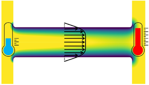
Figure 1. Schematic of a slit nanochannel of length  $l$ and half-height
  $h$, connecting two identical reservoirs at the ends. Generally, a temperature difference
  $\Delta T$ is applied between the reservoirs, as well as a pressure difference
  $\Delta p_0$, an external electric field
  $E$ and a concentration difference
  $\Delta n$. The Debye length
  $\lambda _D$ increases (shrinks) with increasing (decreasing) temperature.
The thickness of the EDL is commonly captured by the dimensionless Debye parameter  $\overline {\kappa }=\kappa h$, where
  $\kappa ^{-1}=\sqrt {\varepsilon_r \varepsilon_0 k_BT/(2Z^2e^2n)} \equiv \lambda _D$ is the Debye length. Here,
  $k_B$,
  $Z$ and
  $e$ represent the Boltzmann constant, the valence of the symmetric electrolyte and elementary charge, respectively. The number concentration of the ions in the bulk, i.e. sufficiently far away from any charged wall, is denoted by
  $n$. The boundary condition for the flow at the channel wall, apart from a vanishing wall-normal velocity, is a Navier slip condition
  $u=\beta ({\partial u}/{\partial \xi })$, where
  $u$ is the
  $x$-velocity,
  $\beta$ is the slip length and
  $\xi$ is the wall-normal coordinate.
In the following subsections, analytical solutions of the governing equations for the thermo-osmotic flow inside the slit channel are derived, assuming an applied pressure difference  $(\Delta p_0)$ combined with a temperature gradient
  $(\Delta T/l)$ and an applied electric field
  $(E)$. To achieve this, a long-wavelength approximation based on the small parameter
  $(A=h/l,\ A\ll 1)$ is employed. This means that all dependent quantities are expanded as power series in
  $A$, and only the leading-order terms are kept. Also, the temperature difference is assumed to be small compared to the reference temperature, i.e.
  $\Delta T/T_0<1$.
2.1. Temperature, electric potential and ion-concentration distributions
The temperature field  $T$ is governed by the energy equation,
  $\rho c_p [\partial _tT+\boldsymbol {u}\boldsymbol {\cdot }\boldsymbol {\nabla }T] = $
  $\boldsymbol {\nabla }\boldsymbol {\cdot }(k\boldsymbol {\nabla } T)$, where Joule heating and viscous dissipation effects are neglected (Dietzel & Hardt Reference Dietzel and Hardt2017). Here,
  $\partial _t\equiv \partial /\partial t$ denotes the partial derivative with respect to time,
  $\boldsymbol {u}\ (=(u,v))$ represents the velocity vector in the
  $(x,y)$ plane, and
  $k$ and
  $c_p$ denote the thermal conductivity and heat capacity of the fluid, respectively. Neglecting the temperature variation of density
  $(\rho =\rho _0)$ and heat capacity
  $(c_p=c_{p,0})$, assuming a linear temperature profile in the
  $X$ direction on the channel walls and considering a symmetry condition along the centre plane
  $Y=0$, one obtains a linear variation of temperature along the
  $X$ direction, i.e.
  $\partial _X\varTheta ={\rm const.}$ and
  $\partial _Y\varTheta =0$, using the long-wavelength approximation (Dietzel & Hardt Reference Dietzel and Hardt2017). Here and in the following, dimensionless variables
  $\tau =tU_0/l$,
  $(X, Y)=(x/l, y/h)$,
  $\varTheta =(T-T_0)/\Delta T$ and
  $(U,V)=(u/U_0,v/AU_0)$ are used, with
  $U_0=\varepsilon_{r,0}\varepsilon_0 (k_B T_0/Ze)^2/\eta _0 h$ being the reference velocity.
Ion transport is assumed to be governed by the Nernst–Planck equation,  $\partial _t n_k + \boldsymbol {\nabla }\boldsymbol {\cdot } [\boldsymbol {u}n_k-D_k\boldsymbol {\nabla } n_k- D_{T,k}n_k\boldsymbol {\nabla } T -D_kn_k(z_ke/k_BT)\boldsymbol {\nabla }\phi ]=0\ (k=1,2)$, which contains advection
  $(\boldsymbol {u}n_k)$, diffusion
  $(-D_k\boldsymbol {\nabla } n_k)$, electromigration
  $(-z_k e D_k n_k \boldsymbol {\nabla } \phi /k_BT)$ and thermodiffusion fluxes
  $(D_{T,k}n_k\boldsymbol {\nabla } T)$. Here,
  $D_k$ represent diffusion coefficients and
  $D_{T,k}$ thermophoretic mobility coefficients, which are associated with intrinsic Soret coefficients via
  $S_k=D_{T,k}/D_k$ (Würger Reference Würger2010). Integrating the Nernst–Planck equations using the long-wavelength approximation with
  $Z_k=z_k/Z$ and
  $N_k=n_k/n_0$, one obtains (Dietzel & Hardt Reference Dietzel and Hardt2017)
 \begin{equation} N_k=N\exp[{-}Z_k\varPsi/(1+\hat{\varTheta}) ]. \end{equation}
Here,  $\hat {\varTheta }=\varTheta \Delta T/T_0$ and, according to the conventional Soret equilibrium,
  $N=\exp (-\overline {S}_0$
  $T_0\hat {\varTheta })$, with
  $\overline {S}_0=(S_1+S_2)/2$ representing the average intrinsic Soret coefficient at
  $T_0$.
Moreover,  $\varPsi$ in (2.1) denotes the dimensionless EDL potential, which in combination with the scaled applied electric potential
  $\varPsi _0$ forms the scaled total electric potential
  $\varPhi$, i.e.
  $\varPhi (X,Y)=\varPsi (X,Y)+\varPsi _0(X)$, with
  $\partial _X\varPsi _0=-\overline {E}$. In all cases, the electric potentials are scaled by the thermal potential
  $(k_BT_0/Ze)$. The total dimensional electric potential
  $\phi$ obeys the Poisson equation
  $\boldsymbol {\nabla }\boldsymbol {\cdot }(\varepsilon_r \varepsilon_0 \boldsymbol {\nabla }\phi )=\rho _f$, with
  $\rho _f=-e\sum _{k=1}^2 z_kn_k$ being the space charge density. Invoking the long-wavelength approximation with the Dirichlet boundary condition
  $\varPsi =\overline {\zeta }=\zeta /(k_BT_0/Ze)$ on the wall
  $Y=1$, and symmetry condition
  $\partial _Y\varPsi =0$ along the centre plane
  $Y=0$, for sufficiently small
  $\zeta$, the EDL potential can derived as
  $\varPsi ^{DH}=\overline {\zeta }[\cosh (\overline {\kappa }Y)/{\cosh (\overline {\kappa })}]$ (Dietzel & Hardt Reference Dietzel and Hardt2017), which is essentially the Debye–Hückel approximation. The spatially varying Debye parameter (
 $\overline {\kappa }$) is related to the standard Debye parameter (
 $\overline {\kappa }_0$) as
  $\overline {\kappa }=\overline {\kappa }_M\sqrt {N/(1+\varTheta \Delta T/T_0)}$, with
  $\overline {\kappa }_M=\overline {\kappa }_0/\sqrt {1+M_0\Delta T\varTheta }$ and
  $M=d_T\varepsilon_r/\varepsilon_r$ (i.e. at
  $T_0$,
  $M_0=d_T\varepsilon_r/\varepsilon_{r,0}$) (Dietzel & Hardt Reference Dietzel and Hardt2017).
2.2. Flow field
While the previous subsection was merely a recapitulation of the results obtained in Dietzel & Hardt (Reference Dietzel and Hardt2017), computing the flow field requires some major deviation from this preliminary work. The reason is that, in Dietzel & Hardt (Reference Dietzel and Hardt2017), the no-slip boundary condition was employed, whereas here a Navier slip condition is assumed at the channel walls. The motion of an incompressible, homogeneous electrolyte solution with a fixed density  $\rho _0$ and a temperature-dependent viscosity
  $\eta$ is governed by the Navier–Stokes equation
  $\rho _0[\partial _t\boldsymbol {u} +\boldsymbol {u}\boldsymbol {\cdot }\boldsymbol {\nabla }\boldsymbol {u}] =-\boldsymbol {\nabla }p + \boldsymbol {\nabla }\boldsymbol {\cdot }\eta [\boldsymbol {\nabla }\boldsymbol {u} +\boldsymbol {\nabla }\boldsymbol {u}^{\rm T}] -\rho _f\boldsymbol {\nabla }\phi -(\Delta T/2)\partial _T (\varepsilon_r \varepsilon_0 ) (\boldsymbol {\nabla }\phi )^2$. The last two terms on the right-hand side correspond to the Korteweg–Helmholtz force (Russel et al. Reference Russel, Russel, Saville and Schowalter1991) obtained from the Maxwell stress tensor.
Now, substituting the expressions for  $\rho _f$ and
  $\phi$, as derived in the previous subsection, the non-dimensional
  $x$- and
  $y$-momentum equations are obtained as
 \begin{align} & A Re [ \partial_{\tau}U+ U\partial_X U + V\partial_Y U] - A^2[ \overline{\eta}\partial_X^2 U+2 \partial_X\overline{\eta}\partial_X U + \partial_Y\overline{\eta}\partial_X V] \nonumber\\ &\qquad -A^2(Ha/\overline{\kappa}_M^2)[ \partial_X^2\varPsi (\partial_X\varPsi-\overline{E}) + (M\Delta T/2)( \partial_X\varPsi-\overline{E} )^2 \partial_X\varTheta] \nonumber\\ &\quad ={-}\partial_X P + \partial_Y( \overline{\eta}\partial_Y U) + (Ha/\overline{\kappa}_M^2)[\partial_Y^2\varPsi (\partial_X\varPsi-\overline{E}) \nonumber\\ &\qquad + M\Delta T \{\partial_Y\varPsi \partial_Y\varTheta (\partial_X\varPsi-\overline{E} ) -\partial_X\varTheta (\partial_Y\varPsi)^2/2 \}] \end{align}
and
 \begin{align} &A^3Re[ \partial_{\tau}V+ U\partial_X V + V\partial_Y V] - A^2[ A^2\overline{\eta}\partial_X^2 V+ \overline{\eta}\partial_Y^2 V + A^2\partial_X\overline{\eta} \partial_X V + 2\partial_Y\overline{\eta}\partial_Y V\nonumber\\ &\qquad + \partial_X\overline{\eta} \partial_Y U ] -A^2(Ha/\overline{\kappa}_M^2) [ \partial_X^2\varPsi \partial_Y\varPsi + M\Delta T \{ ( \partial_X\varPsi-\overline{E}) \partial_Y\varPsi \partial_X\varTheta \nonumber\\ &\qquad - ( \partial_X\varPsi-\overline{E} )^2\partial_Y\varTheta/2 \}] \nonumber\\ &\quad ={-} \partial_Y P + (Ha/\overline{\kappa}_M^2)[ \partial_Y^2\varPsi \partial_Y\varPsi + M\Delta T (\partial_Y\varPsi)^2 \partial_Y\varTheta/2 ]. \end{align}
 In these equations, a number of dimensionless parameters are encountered, most notably the Reynolds number  $Re=\rho _0U_0h/\eta _0$ and the Hartmann number
  $Ha=2Ahn_0k_BT_0/U_0\eta _0$, where
  $\eta _0$ stands for the viscosity of the fluid at temperature
  $T_0$, which provides the scale for the non-dimensional viscosity
  $\overline {\eta }=\eta /\eta _0$. The Hartmann number compares the velocity scale due to osmotic pressure with the reference velocity. The pressure is scaled as
  $P=p/(U_0\eta _0/Ah)$. In accordance with the long-wavelength approximation we can neglect terms of
  ${O}(A^2)$ or higher. Also, we can neglect terms of
  ${O}(ARe)$ or higher, since we assume
  $Re\ll 1$, as characteristic for nano- and microscale flows.
Making use of the Poisson equation in (2.3), one obtains  $\partial _Y[P-Ha(1+\hat {\varTheta })(N_++N_-)/2]=0$. Integrating this with respect to the
  $Y$-coordinate and using the Debye–Hückel approximation yields
  $[P-Ha(1+\hat {\varTheta })N]=f(X)$. Here, the second term on the left-hand side represents the osmotic pressure due to the ion cloud, which leaves
  $f(X)$ as the externally applied pressure
  $P_0(X)$. Thus, the pressure can be rewritten as
  $P=P_0+Ha N(1+\hat {\varTheta })[ \cosh (\varPsi /(1+\hat {\varTheta }))-1]$, which yields
  $\partial _XP=d_XP_0 + (Ha/2)\partial _X\hat {\varTheta }(N/(1+\hat {\varTheta }))[\varPsi ^2 (\partial _{\hat {\varTheta }}N/N) +2\varPsi \partial _{\hat {\varTheta }}\varPsi -\varPsi ^2/(1+\hat {\varTheta })]$ using the Debye–Hückel approximation. Here,
  ${\rm d}_X\equiv {\rm d}/{\rm d}X$ represents the ordinary derivative with respect to
  $X$. On the other hand, employing
  $\partial _Y\varTheta =0$ and
  $N/(1+\hat {\varTheta })=(\overline {\kappa }/\overline {\kappa }_M)^2$, and substituting
  $\partial _XP$ in (2.2) gives
 \begin{align} \partial_Y(\overline{\eta}\partial_Y U) &=d_X P_0 + \frac{Ha}{\overline{\kappa}_M^2}\overline{E} \partial_Y^2\varPsi +\frac{Ha}{2\overline{\kappa}_M^2}\partial_X\hat{\varTheta} \left[ \overline{\kappa}^2 \left\{ \frac{\partial_{\hat{\varTheta}}N}{N}-\frac{1}{1+\hat{\varTheta}} \right\}\varPsi^2\right.\nonumber\\ &\quad \left.+\, MT_0\left( \partial_Y\varPsi \right)^2 + 2\overline{\kappa}\left( \frac{\partial_{\hat{\varTheta}}\overline{\kappa}}{\overline{\kappa}} \right) \{ \overline{\kappa}^2\varPsi -\partial_Y^2\varPsi \} \partial_{\overline{\kappa}}\varPsi \right]. \end{align}
The last term of (2.4) vanishes under the Debye–Hückel approximation.
The viscosity of a binary aqueous electrolyte solution containing small ions primarily depends on temperature and on ion concentration. As per the assumption, the latter does not play a significant role here, since the Nernst–Planck equation used in this work implicitly requires low enough ion concentrations. In accordance with the spatial variation of temperature in the present analysis, viscosity can be considered to depend exclusively on  $X$. Without knowing the explicit distribution of viscosity, (2.4) can be integrated twice with respect to
  $Y$, and employing
  $\partial _YU=0$ at
  $Y=0$, and Navier slip on the wall, i.e.
  $U=-\overline {\beta }\partial _Y U$ at
  $Y=1$, one has
 \begin{align} U&=\frac{1}{2\overline{\eta}}d_XP_0[Y^2-1 -2\overline{\beta}] +\frac{Ha}{\overline{\eta}\overline{\kappa}_M^2}\overline{E}\overline{\zeta} \left[ \frac{ \cosh(\overline{\kappa}Y) }{\cosh(\overline{\kappa})} -1 -\overline{\beta}~\overline{\kappa}\tanh(\overline{\kappa})\right] \nonumber\\ &\quad +\frac{Ha}{\overline{\eta}\overline{\kappa}_M^2} \frac{\partial_X\varTheta\overline{\zeta}^2}{8\cosh^2{(\overline{\kappa})}} \left[ \left(\frac{\partial_{\hat{\varTheta}}N}{N} -\frac{1}{1+\hat{\varTheta}} +MT_0\right) \left(\frac{\cosh(2\overline{\kappa}Y) - \cosh(2\overline{\kappa})}{2}\right.\right.\nonumber\\ &\left.\left.\quad -\,\overline{\beta}\overline{\kappa}\sinh(2\overline{\kappa}) \vphantom{\frac{\partial_{\hat{\varTheta}}N}{N}}\right) + \overline{\kappa}^2\left(\frac{\partial_{\hat{\varTheta}}N}{N} -\frac{1}{1+\hat{\varTheta}} -MT_0\right) (Y^2-1-2\overline{\beta})\right], \end{align}
with  $\overline {\beta } = \beta / h$.
Equation (2.5) describes the scaled axial velocity under the influence of an external pressure gradient ( $d_XP_0$), applied electric field (
 $\overline {E}$) and axial temperature gradient (
 $\partial _X\hat {\varTheta }$) with a finite slip length
  $\beta$ on the channel wall. Equation (2.5) takes into account the axial concentration gradient
  $(\partial _{\hat {\varTheta }}N/N)$ due to the Soret equilibrium, i.e.
  $\partial _{\hat {\varTheta }}N/N=-\overline {S}_0T_0$. This means that, in the framework of our analysis, the axial concentration gradient is solely due to the applied temperature gradient, i.e. it is not an independent quantity. In the absence of a temperature gradient and at vanishing slip length, (2.5) reduces to the well-known expression for superposed electro-osmotic and pressure-driven flow (Dietzel & Hardt Reference Dietzel and Hardt2017).
However, substituting  $\overline {\beta }=0$ in (2.5) does not lead us to the corresponding TOF velocity profile developed by Dietzel & Hardt (Reference Dietzel and Hardt2017). The reason is that the expression for the osmotic pressure derived in Dietzel & Hardt (Reference Dietzel and Hardt2017) is not valid for overlapping EDLs. By integrating (2.5) across the channel cross-section, we obtain the volume flux within the Debye–Hückel limit as
 \begin{align} \frac{Q}{\Delta z (2h)U_0}&={-}\frac{1}{\overline{\eta}}d_XP_0\left[\frac{1}{3} +\overline{\beta}\right] +\frac{Ha}{\overline{\eta}\overline{\kappa}_M^2}\overline{E}\overline{\zeta} \left[ \frac{ \tanh(\overline{\kappa}) }{ \overline{\kappa}} -1 -\overline{\beta}\overline{\kappa}\tanh(\overline{\kappa})\right]\nonumber\\ &\quad +\frac{Ha}{\overline{\eta}\overline{\kappa}_M^2} \frac{\partial_X\varTheta\overline{\zeta}^2}{8\cosh^2{(\overline{\kappa})}} \left[ \left( \frac{\partial_{\hat{\varTheta}}N}{N} -\frac{1}{1+\hat{\varTheta}} +MT_0\right) \left( \frac{\sinh(2\overline{\kappa})}{4\overline{\kappa}} - \frac{\cosh(2\overline{\kappa})}{2}\right.\right.\nonumber\\ &\left.\left.\quad -\,\overline{\beta}\overline{\kappa}\sinh(2\overline{\kappa}) \vphantom{\frac{\partial_{\hat{\varTheta}}N}{N}}\right) - 2\overline{\kappa}^2\left( \frac{\partial_{\hat{\varTheta}}N}{N}-\frac{1}{1+\hat{\varTheta}} -MT_0\right)\left( \frac{1}{3}+ \overline{\beta}\right)\right]. \end{align}
As  $\overline {\kappa }\to \infty$ and in the absence of
  $d_XP_0$,
  $\overline {E}$ and
  $\overline {\beta }$, the right-hand side of (2.6) approaches
  $-(Ha/8\overline {\eta }\overline {\kappa }_M^2)\partial _X\varTheta \overline {\zeta }^2(\partial _{\hat {\varTheta }}N/N - 1/(1+\hat {\varTheta }) +MT_0)$, which is identical to the corresponding solution derived by Dietzel & Hardt (Reference Dietzel and Hardt2017).
The physics underlying thermo-osmotic fluid propulsion was already discussed in detail by Dietzel & Hardt (Reference Dietzel and Hardt2017). Briefly, in thermal equilibrium, the electrostatic force on the ion cloud in the Debye layer and the force due to the osmotic pressure exactly cancel, leaving the entire liquid in local mechanical equilibrium. However, in the situation considered here, temperature gradients result in a deviation from thermal equilibrium, which means that the electrostatic and osmotic pressure forces no longer cancel. This induces a driving force, which is the origin of thermo-osmotic propulsion.
3. Analysis and discussion of specific cases
This section serves two different purposes. The main focus of the first subsection is to explore the accuracy and the limits of validity of our analytical solution by comparison with numerical results. The second subsection is devoted to making predictions for the TOF through realistic nanochannels, with special consideration of the coupling between surface charge and slip length. In all cases we solely consider the response of the system to an axial temperature gradient, i.e. without any applied pressure gradient or electric field.
To numerically compute the TOF inside the nanochannel, the Poisson, Nernst–Planck, Navier–Stokes and heat transfer equations were solved using the finite-element framework of COMSOL Multiphysics 6.1. Quadratic elements were employed for the electric potential, concentration, temperature and velocity fields, and linear elements for the pressure field. The computational domain was discretized with a structured grid. The grid independence of the numerical solutions was verified using systematic grid refinement and Richardson extrapolation to estimate the grid-independent result. The total volume flux through the channel was chosen as the representative value for grid-quality assessment, and the relative error between a numerically computed and the extrapolated value was required to fall below  $10^{-3}$.
3.1. TOF within a charged nanochannel with a fixed slip length
Fundamentally, there are three different mechanisms that drive the flow due to an axial temperature gradient ( $\partial _X\hat {\varTheta }$) (Dietzel & Hardt Reference Dietzel and Hardt2017): these are the temperature-dependent ratio between the diffusivity and the electrophoretic mobility of the ions (the Einstein–Smoluchowski relation), the temperature-dependent dielectric permittivity of the fluid and the thermophoretic ion motion. The latter is incorporated in terms of the Soret coefficient (
 $\overline {S}_0$), creating an axial concentration gradient in the nanochannel, which in turn causes diffusio-osmosis (Marbach & Bocquet Reference Marbach and Bocquet2019). To obtain a quantitative measure of this contribution to the TOF, we consider
  $\overline {S}_0=1\times 10^{-3}~{\rm K}^{-1}$ (Dietzel & Hardt Reference Dietzel and Hardt2017), which represents a characteristic order of magnitude for small ions. Figure 2(a) shows that, without any thermophoretic ion motion, the centreline velocity gets reduced by approximately 24 % (12 %) at
  $\kappa _0h=1$ (
 $\kappa _0h=10$). In all results to be presented in the following, thermophoretic ion motion with
  $\overline {S}_0=1\times 10^{-3}$ K
 $^{-1}$ is included.

Figure 2. (a) Analytical (2.5) (solid lines) and numerical (symbols) TOF velocity profiles for  $\overline {S}_0=0$ and
  $10^{-3}~{\rm K}^{-1}$ at
  $\beta =0$ nm. (b) Interfacial thickness
  $\lambda _0/h$ (3.1) for TOF within a slit channel (solid line) and interfacial thickness
  $(1/2\kappa h)$ for TOF over a planar surface (dashed line) as a function of
  $\kappa h\ (=\overline {\kappa })$. (c–f) Analytical (2.5) (solid lines) and numerical (dashed lines with symbols) TOF velocity profiles for different values of (c)
  $\kappa _0h$, (d)
  $\beta$, (e)
  $\zeta$ and (f)
  $\Delta T$. Unless otherwise specified, the other parameters are fixed to
  $\zeta =-15$ mV,
  $\beta =0.1$ nm,
  $\kappa _0h=10$,
  $\Delta T=25$ K,
  $l=100\times 2h$,
  $h=5$ nm,
  $\overline {\eta }=1$,
  $\overline {S}_0=10^{-3}$ K
 $^{-1}$ and
  $M_0=-5.1\times 10^{-3}$ K
 $^{-1}$. The parameters are varied within a range that can be considered practically feasible according to literature data (Joly et al. Reference Joly, Ybert, Trizac and Bocquet2004; Masliyah & Bhattacharjee Reference Masliyah and Bhattacharjee2006; Balme et al. Reference Balme, Picaud, Manghi, Palmeri, Bechelany, Cabello-Aguilar, Abou-Chaaya, Miele, Balanzat and Janot2015; He et al. Reference He, Tsutsui, Miao and Taniguchi2015; Chen, Yao & Su Reference Chen, Yao and Su2019; Xie et al. Reference Xie, Fu, Niehaus and Joly2020). Velocity profiles are obtained at the middle cross-section of the nanochannel.
Figure 2(c–f) shows the (dimensional) analytical and numerical profiles for various values of the Debye parameter, slip length, wall zeta potential and temperature difference. Figure 2(c) displays the variation of the velocity profile with  $\kappa _0h$. The curves essentially cover the transition from overlapping EDLs to thin EDLs. The TOF velocity gradually increases as the EDL becomes thinner and eventually the profile attains a plug-like shape for higher values of
  $\kappa _0h$. For the corresponding small value of
  $\zeta$, an excellent agreement between the analytical and numerical results is observed for all considered values of
  $\kappa _0h$.
Figure 2(d) illustrates the impact of the slip length on the TOF velocity. The maximum slip length (40 nm) is close to the value typically encountered for an uncharged graphene surface (Xie et al. Reference Xie, Fu, Niehaus and Joly2020). Generally, we expect material-specific relationships between the surface charge and the slip length, similar to those reported in Xie et al. (Reference Xie, Fu, Niehaus and Joly2020). However, in this section, the  $\zeta$ potential and the slip length are regarded as independent parameters to render the problem analytically tractable. Without losing generality, going beyond such an approximation would require a universal relationship between the surface charge and the slip length, which we are not aware of. In figure 2(d), a distinct increase of the velocity with the slip length is visible. The results indicate a good agreement between the analytical and the numerical velocity profiles at low to moderate slip length values, beyond which the analytical velocity overestimates the values obtained from the numerical simulations. The reason behind these deviations is due to entrance effects. With increasing slip length, entrance effects become more and more prominent, and it becomes increasingly difficult to reproduce the results characteristic for a fully developed flow profile with a channel of finite length, as represented through the computational domain of our numerical simulations.
The enhancement of surface-driven transport by boundary slip was rationalized in Ajdari & Bocquet (Reference Ajdari and Bocquet2006) for a surface bounded by an infinite half-space, where it was shown that the effective slip velocity scales as  $(1+\beta /\lambda )$, with
  $\lambda$ being an interface thickness parameter (
 $\lambda _{EOF}\sim 1/\kappa,\ \lambda _{DOF}\sim 1/2\kappa$ for the case of electro-osmotic (EOF) and diffusio-osmotic (DOF) flow, respectively). In our case, we can take the velocity at the channel centre plane
  $v_s^0$ as a measure of flow enhancement. We analytically obtain flow enhancement by a factor of
  $(1+\beta /\lambda _0)$, where the dimensionless interfacial thickness
  $\lambda _0/h$ is given as
 \begin{equation} \lambda_0/h= \dfrac{\left( \dfrac{\partial_{\hat{\varTheta}}N}{N} - \dfrac{1}{1+\hat{\varTheta}} -MT_0 \right)\overline{\kappa}^2+\left( \dfrac{\partial_{\hat{\varTheta}}N}{N} - \dfrac{1}{1+\hat{\varTheta}} +MT_0 \right)\sinh^2{(\overline{\kappa})}}{\left( \dfrac{\partial_{\hat{\varTheta}}N}{N} - \dfrac{1}{1+\hat{\varTheta}} -MT_0 \right)2\overline{\kappa}^2+\left( \dfrac{\partial_{\hat{\varTheta}}N}{N} - \dfrac{1}{1+\hat{\varTheta}} +MT_0 \right)\overline{\kappa}\sinh(2\overline{\kappa})}. \end{equation}
 As  $\overline {\kappa }$ tends to infinity,
  $\lambda _0$ approaches
  $1/2\kappa$ (cf. figure 2b), which is the corresponding interfacial length for diffusio-osmotic flow identified in Ajdari & Bocquet (Reference Ajdari and Bocquet2006). Equation (3.1) represents a generalization of the results reported in Ajdari & Bocquet (Reference Ajdari and Bocquet2006) and provides a simple means to estimate the flow velocity scale related to a specific value of the slip length. Figure 2(d) reveals a quantitative measure of the flow enhancement due to boundary slip. For
  $\beta =40$ nm, the analytically determined velocity
  $v_s^0$ exhibits an enhancement of
  ${\sim }161$ times relative to the no-slip case.
The results depicted in figure 2(e,f) manifest the influence of the  $\zeta$ potential and the temperature gradient on the TOF. Figure 2(e) reveals that the velocity magnitude is proportional to the magnitude of the
  $\zeta$ potential, as for electro-osmotic flow. The increasing discrepancies between the analytical and the numerical solutions at higher
  $\zeta$ potentials are attributed to the fact that the analytical results were derived under the Debye–Hückel approximation. Similarly, the curves in figure 2(f) evidence a good agreement between the analytical and the numerical results for a sufficiently small temperature gradient, i.e.
  $\Delta T/T_0\approx 0.1$. This is due to the fact that the long-wavelength approximation was applied in deriving the flow field, which translates to the assumption of local thermal equilibrium at each position in the channel (
 $|\Delta T/T_0|\ll 1$). For large applied temperature gradients, this assumption will be violated.
3.2. TOF between polarized graphene surfaces
In this section, we analyse a specific case to demonstrate how large the flow augmentation due to boundary slip can become in realistic scenarios. For this purpose, we need to consider the relationship between the slip length and the charge density at the walls. Given a fixed  $\zeta$ potential at the channel walls, we arrive an axially varying charge density. The reason is that the scale of the wall charge density is given by
  $\zeta$ divided by the Debye length, which exhibits an axial variation because of the temperature dependence of the Debye length. Specifically, we examine the case of a channel bounded by charged graphene walls, for which the slip length–charge density relationship was reported in Xie et al. (Reference Xie, Fu, Niehaus and Joly2020).
Therefore, unlike in the previous scenarios with a uniform slip length along the channel wall, here we encounter an axially varying slip length. The analytical model fails to capture the corresponding flow field, which is why the results of this subsection were solely obtained using finite-element simulations.
In order to model the TOF inside a slit nanochannel with polarized graphene walls, we follow an iterative procedure, where the entire system of Poisson, Nernst–Planck and Navier–Stokes equations is numerically solved at each iteration step. Initially we consider a fixed  $\zeta$ potential, i.e.
  $\zeta _0$, which corresponds to a fixed surface charge density
  $\sigma _0$ through the Grahame equation (Israelachvili Reference Israelachvili2011). Invoking the slip–charge relation (Xie et al. Reference Xie, Fu, Niehaus and Joly2020), we obtain a fixed slip length
  $\beta _0$ corresponding to
  $\sigma _0$. We initiate the iteration with a fixed pair
  $(\zeta _0,\beta _0)$. Based on that, we numerically solve for the TOF, resulting in an axially varying surface charge density
  $\sigma _1(x)$, which is due to the temperature dependence of the Debye length. The spatially varying surface charge densities
  $\sigma _n(x)\ (n\geq 1)$ lead us to axially varying slip lengths
  $\beta _n(x)\ (n\geq 1)$ (Xie et al. Reference Xie, Fu, Niehaus and Joly2020) at each iteration step. We repeat the iteration procedure until the difference between
  $\sigma _n(x)$ and
  $\sigma _{n+1}(x)$ becomes less than
  $0.1\,\%$.
The TOF velocity profiles obtained from the converged solutions are displayed in figure 3. The profiles are evaluated at a cross-section at the centre of the nanochannel, and the specific form of these profiles is attributed to the locally varying slip length  $\beta (x)$. The non-uniform slip length results in an axial variation of the flow resistance. To ensure mass conservation, an adverse pressure-driven flow builds up, which in combination with the TOF results in non-monotonic velocity profiles. As apparent from figure 3, for a
  $\zeta$ potential of
  $-20$ mV, TOF velocities as high as
  ${\sim }1.6~{\rm mm}~{\rm s}^{-1}$ are obtained. Compared to a nanochannel with no-slip walls and considering a salt concentration of 1.3 M (0.13 M), we obtain a flow velocity enhancement of
  ${\sim }200\ (78)$ times and of
  ${\sim }250\ (80)$ times, corresponding to
  $\zeta _0=-20$ mV and
  $-5$ mV, respectively.

Figure 3. Numerically obtained TOF axial velocity profiles between polarized graphene walls, corresponding to  $\zeta _0=-5,\ -10,\ -15$ and
  $-20$ mV. The other parameters are
  $c_0=0.13$ M (
 $\kappa _0 h\approx 6$) and
  $1.3$ M (
 $\kappa _0 h\approx 19$),
  $\Delta T=25$ K,
  $l=100\times 2h$ and
  $h=5$ nm. Velocity profiles are obtained at the middle cross-section of the nanochannel.
4. Discussion, conclusion and outlook
In this article, we have derived an analytical expression for the thermo-osmotic flow in a slit channel with boundary slip based on a continuum mechanical framework and the Debye–Hückel approximation. The expression accounts for the additional effects of an applied pressure gradient and an applied electric field. The analytical results for the flow profile agree well with numerical results within the range of validity of the approximations employed. To demonstrate the flow augmentation due to boundary slip, we have considered the TOF between homogeneously charged graphene walls as a special case. Compared to a channel with no-slip walls, a flow augmentation by more than two orders of magnitude was found, which demonstrates the massive effects that boundary slip may have on TOF.
Especially for narrow channels, the question arises how accurate a model may be that is solely based on a continuum mechanical framework. Clearly, our model does not account for effects occurring on the molecular level in the utmost vicinity of the solid–liquid interface. Close to the interface, the enthalpy density of the liquid will deviate from the enthalpy density away from the interface, which determines the solid–liquid interfacial tension. It was shown that this excess enthalpy can drive a thermoelectric response in nanochannels (Fu, Joly & Merabia Reference Fu, Joly and Merabia2019). At least in narrow channels, the excess enthalpy close to the solid–liquid interface is an effect that needs to be considered in addition to the effects that have been included in our continuum mechanical model. It is expected that the excess enthalpy is characteristic of the specific solid–liquid combination, i.e. finding a universal expression for this contribution appears to be out of reach. By contrast, what we have considered in the present work is a rather universal effect that plays a role in a broad class of scenarios, i.e. dilute electrolyte solutions confined between walls with a low to moderate surface charge density. In the future, the goal will be to formulate a more complete description that takes into account the effects occurring on the continuum scale as well as the specific molecular effects at the solid–liquid interface.
Acknowledgements
Fruitful discussions with L. Joly and S. Merabia are gratefully acknowledged.
Funding
Financial support by the German Research Foundation (DFG), project ID HA 2696/52-1 is gratefully acknowledged.
Declaration of interests
The authors report no conflict of interest.


