


Introduction
CuNi alloys are well-known materials in industry and therefore well investigated. Because of their high corrosion resistance, low macrofouling rates, and good fabricability, they are a good candidate for marine applications like naval condensers and piping. Furthermore, their ductility at low temperatures makes them interesting for components in cryogenic processing and storage compounds (CDA, 2020). CuNi nanoparticles are interesting for their catalytic use in carbon oxide reduction and for the growth of graphene mono- and bilayers (Panizon et al., Reference Panizon, Olmos-Asar, Peressi and Ferrando2015).
Regarding the phase diagram, however, a miscibility gap at temperatures below 773 K is controversially discussed. The determination of phase boundaries is not an easy task since the diffusivity is very slow at the considered temperatures and phase equilibrium can only be reached with extremely long annealing times (Johnson et al., Reference Johnson, Bauer and Jordan1986). Nevertheless, some attempts were made to clarify this issue by indirect experimental measurements and by computational methods which all support the phase separation tendency and the existence of a miscibility gap (Vrijen & Radelaar, Reference Vrijen and Radelaar1978; Tomiska & Neckel, Reference Tomiska and Neckel1984; Srikanth & Jacob, Reference Srikanth and Jacob1989; Asta & Foiles, Reference Asta and Foiles1996). The reports, however, show large discrepancies with respect to critical temperature T C and the exact position of the binodal line. To overcome this, direct experimental analysis of the phase boundary composition must be realized. The main difficulties are achieving thermodynamic equilibrium in reasonable times and using high-resolution composition sensitive measurements.
In this work, the annealing times were reduced by using thin films of just a few nanometers to shorten the necessary diffusion length. The statistical significance is increased by using multilayered diffusion couples with 10 or 20 layers of each. To make sure to be in thermodynamic equilibrium within the selected annealing times, an effective interdiffusion coefficient D eff was determined, which describes the diffusion in both directions, Cu into Ni and Ni into Cu, and includes all kinds of defect transport of the nanocrystalline microstructure, like grain boundary- and dislocation diffusion.
Since grain boundary wetting or interface roughness could be misinterpreted as interdiffusion when using depth profiling with poor lateral resolution, microscopic analysis by atom probe tomography (APT) was performed to characterize the thin film model system. This technique is particularly qualified for its outstanding resolution in the nanometer range and chemical analysis at the same time. Additionally, with the three-dimensional reconstruction, microstructure development can be investigated, which is of great importance here, since some works indicate that Ni-rich and Cu-rich clusters are possible (Gupta et al., Reference Gupta, Cheng and Beck1964; Pawel & Stansbury, Reference Pawel and Stansbury1965; Mozer et al., Reference Mozer, Keating and Moss1968; Vrijen & Radelaar, Reference Vrijen and Radelaar1978; Wagner et al., Reference Wagner, Poerschke and Wollenberger1982). Similar APT experiments on multilayered thin films were already carried out in works of Stender et al. (Reference Stender, Balogh and Schmitz2011) to investigate thermal stability of GMR sensors (Fe/Cr) or analyzing spinodal decomposition in TiAlN/CrN (Povstugar et al., Reference Povstugar, Choi, Tytko, Ahn and Raabe2013).
Materials and Methods
Suitable samples were prepared by electropolishing a coarse-grained W-wire of 75 μm diameter in a 1 M NaOH electrolyte solution using a graphite counter electrode to receive needle-shaped tips with a nanometer-sized apex diameter. The tips were further shaped using focused ion beam (FIB) to cut a planar end surface of around 2 μm in diameter (Stender et al., Reference Stender, Balogh and Schmitz2011).
On these posts, CuNi multilayers were coated using a custom-built ion beam sputtering (IBS) chamber. The multilayers consist of 10 or 20 layers of each material and a cap of pure Ni to protect the samples against oxidation. As layer materials, pure Cu, and alloyed Ni with 30 at% Cu were used. According to the literature, diffusion of Cu into Ni and vice versa show a huge difference [D Ni in Cu = 1.80 × 10⁻²¹ m 2/s and D Cu in Ni = 3.32 × 10⁻²⁴ m2/s for T = 623 K, according to Johnson et al. (Reference Johnson, Bauer and Jordan1986)]. By pre-alloying the Ni layers, the slow diffusivity of Cu into Ni is partly compensated to reduce the contrast in diffusivities and thus to reach equilibrium in experimentally achievable times (Thomas & Ernest Birchenall, Reference Thomas and Ernest Birchenall1952; Arnould & Hild, Reference Arnould and Hild2002; Wierzba & Skibiński, Reference Wierzba and Skibiński2016). The layer thicknesses were chosen to achieve an average concentration of 50 at% for each component, that is, 3 nm of Cu and 8 nm of Ni0.7Cu0.3 (Fig. 1a). To calibrate the thickness monitor of the sputter device, a TEM image from multilayers with 10 nm single layer thickness was taken. For that, a SiO2 plate has been coated first with one layer CuNi, 25 nm in thickness as a buffer layer, then 10 bilayers of (Cu10nm/Ni10nm). To protect the layers during FIB milling, an additional 500 nm Cr layer was sputtered. Finally, a lamella of this sample was cut through the standard FIB lift-out process. In Figures 1b and 1c, typical results of the produced microstructure are shown. Although the two metals show nearly no material contrast, the layers can be partly distinguished from the structural interfaces. Layers are planar and in good agreement with the aimed thicknesses. In Figure 1c, a low magnification image is shown as an overview. The colored regions show individual grains determined with dark-field imaging. They have columnar morphology with a lateral diameter of around 25 nm and spread across multiple layers indicating coherent interfaces. Since no chemical contrast is observed, an EDX mapping is recorded with a spot size of 4 nm, as shown in the inset of Figure 1c. Here, the alternating Cu (pink) and Ni (yellow) layers are clearly visible.
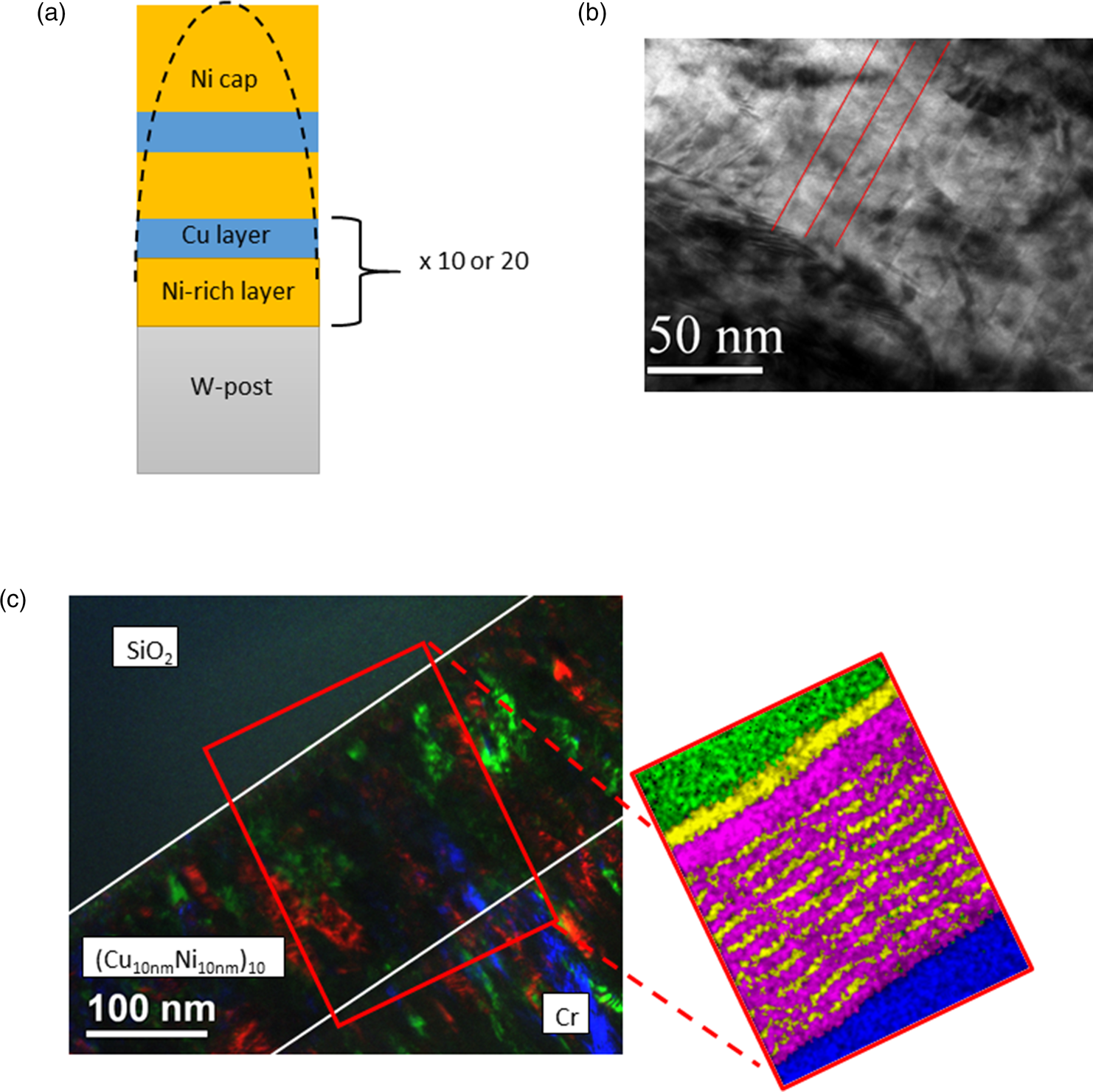
Fig. 1. (a) Schematic illustration of the sample tip. (b) Cross-section TEM image of the multilayer showing that the correct layer thicknesses of around 10 nm per layer has been achieved. (c) Colored overlay of different dark-field images of the same lamella. The colored regions mark grains, which obviously spread through the whole layer system. The chemical layer structure is proven by EDX mapping as shown on the right-hand side.
The layer systems on W posts were annealed in a UHV furnace with a residual pressure of <1 × 10⁻⁷ mbar. The annealing treatments were performed at 573, 623, and 673 K. For each temperature, different annealing durations were carried out, as summarized in Table 1.
Table 1. Used annealing times and temperatures.
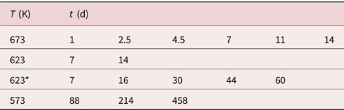
623* has different starting concentrations of c 2 = 0.7 and c 1 = 0.44.
After annealing, the samples were sharpened by annular milling (Prosa & Larson, Reference Prosa and Larson2017) and measured by a custom-built, laser-assisted APT with a pulsing rate of 200 kHz and a pulse energy of around 150 nJ at a base temperature of 60 K (Schlesiger et al., Reference Schlesiger, Oberdorfer, Würz, Greiwe, Stender, Artmeier, Pelka, Spaleck and Schmitz2010). Cu and Ni are detected mainly in the single charged state with no overlapping mass peaks (see Fig. 2 for an exemplary mass spectrum and Supplementary material for exact peak identification). For the volume reconstruction, the protocol from Bas et al. (Reference Bas, Bostel, Deconihout and Blavette1995), which relies on the point projection model, and a geometrical algorithm to determine the tip radius according to Jeske & Schmitz (Reference Jeske and Schmitz2001) were used. To calibrate the reconstruction, the lattice plane distances in Cu and Ni layers were adjusted to their theoretical values.
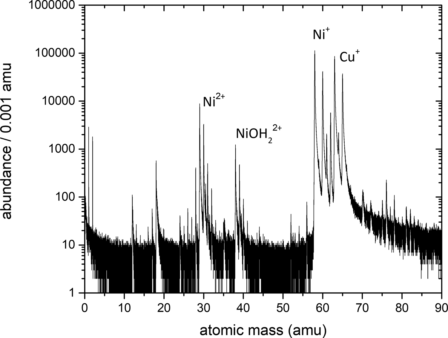
Fig. 2. Exemplary mass spectrum from an atom probe analysis of a sample annealed at 673 K for 2.5 d. The exact peak identification can be found in the Supplementary material.
Results
The suitability of the procedure was tested first. To make sure that the layers are created as planned and their concentrations can be measured, an as-prepared sample is analyzed. The volume reconstruction of the tip and a 1D composition profile from a small probing cylinder are shown in Figure 3. The different layers are nearly straight and can be distinguished easily. The reconstruction also shows that the thin Cu layers become narrower at the outside and thicker in the middle. This effect is due to reconstruction artifacts caused by the lower evaporation field of Cu (30 V/nm) in comparison to Ni (35 V/nm). Quantitative analysis is made by 1D composition profiles (Fig. 3b) using a rectangular box perpendicular orientated to the interfaces with a probing volume of 10 × 10 × 80 nm3. Several box sizes and tip regions were tested to find the profile with the best resolution. The Cu compositions of the layers are (30 ± 1.4) at% and 100 at% and the layer thicknesses are in accordance with the desired sputtered size. Maximum thickness fluctuations of around 2 nm occur, either caused by sputtering errors or by reconstruction artifacts. Nevertheless, this layer roughness does not affect the equilibrium composition and is therefore of minor interest here.
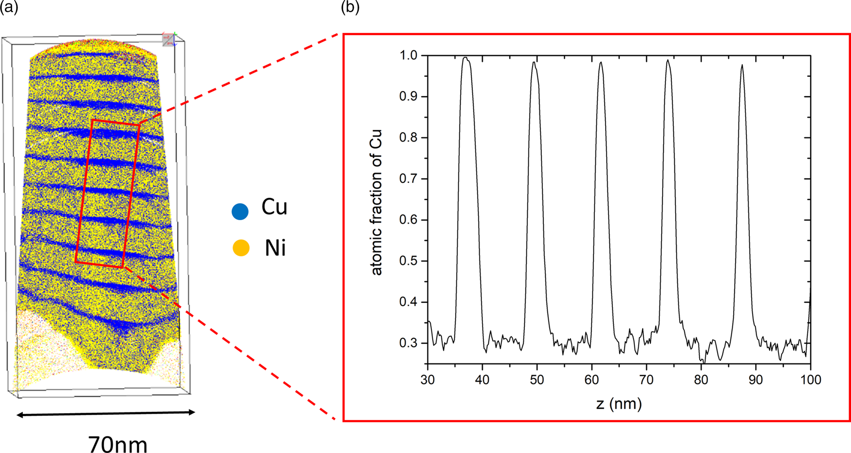
Fig. 3. (a) Cross-section of an as-prepared sample (the low density “triangles” at the bottom are due to the strong contrast of evaporation threshold between Ni and tungsten) and (b) its concentration profile for Cu along the tip axis.
Microstructural Development
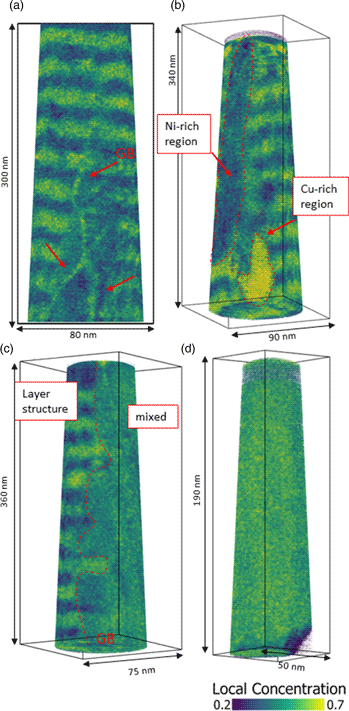
During annealing for different durations, diffusive transport changes the layer structure of the samples until it is fully homogenized or the compositions of heterogeneous phases match the solubility limits. If the annealing time is not sufficient to reach equilibrium, intermediate states will be formed. In Figure 4, tip reconstructions of annealed samples at 673 K for 2.5 d (Fig. 4c) and 4.5 d (Figs. 4a, 4b, 4d) with typical observed microstructures are shown. In Figure 4a, the layer structure is still intact, however, three grain boundaries are visible (red arrows), differing in their composition (60 at% Cu) by segregation from the layers, while the surrounding layer structure is eliminated to an average concentration of around 35 at% Cu. Because of their defective structure, grain boundaries are fast diffusion paths to reach the local equilibrium faster or to provide heterogeneous nucleation sites. During the mixing process, composition fluctuations including precipitate-like volumes of increased concentration will occur as shown in Figure 4b (regions are framed by red dashed line) with concentrations of 29 at% (Ni-rich) and 73 at% of Cu. Often an asymmetric situation is observed where on one side of the grain boundary still the layer system is intact while on the other side full mixing is observed (c Cu = 48 at%, Fig. 4c). This geometrical situation indicates mixing by diffusion induced grain boundary migration (DIGM) as suggested for very low temperatures (King, Reference King1987). Finally, the whole specimen appears to be completely mixed (Fig. 4d).
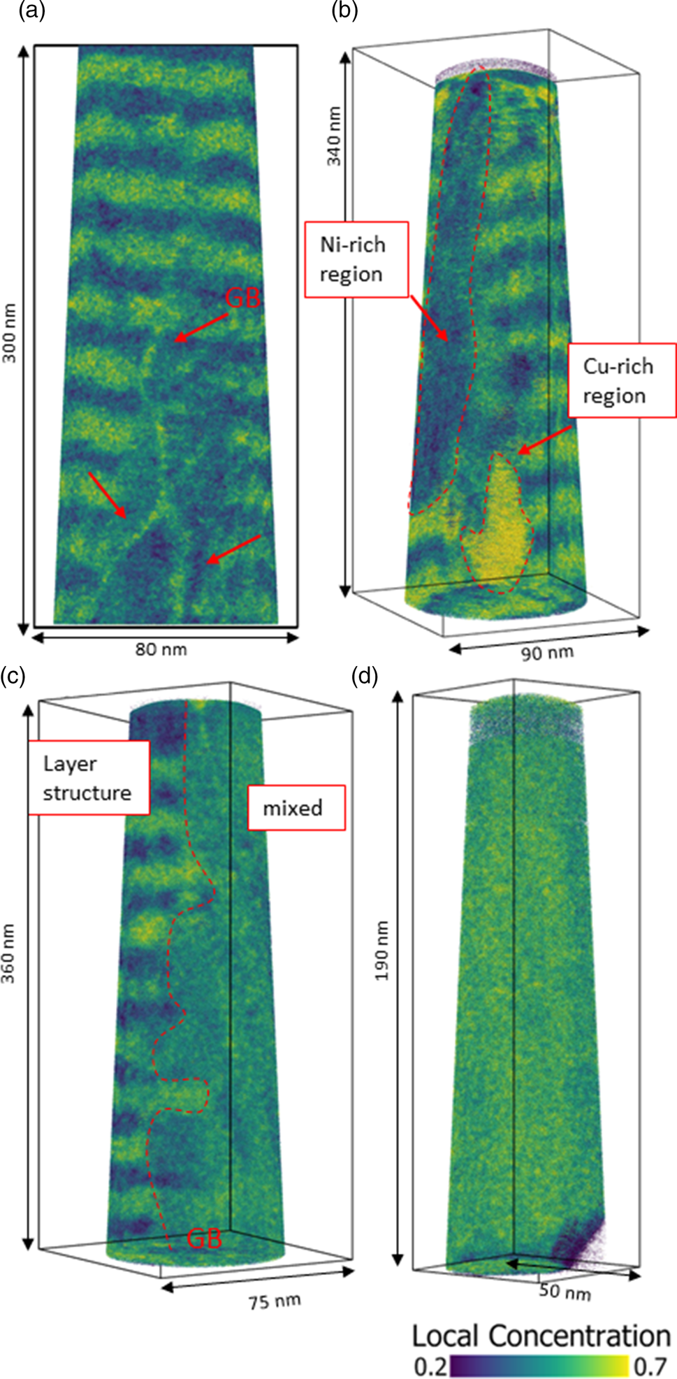
Fig. 4. Local Cu concentration plots of tips annealed at 673 K. Microstructural development of mixing shown at different states. In (a), mixing starts in grain boundaries of a sample annealed for 4.5 d. (b) Nucleation and growth cause composition fluctuations in bulk (annealed for 2.5 d). (c) Diffusion induced grain boundary migration in a sample annealed for 4.5 d. And (d) total mixing of a sample annealed for 4.5 d.
An interesting point is that the intermediate states show pronounced variation although annealing time and temperature were kept almost constant. The reason is, that in the kinetic regime, the microstructure is crucial. Since grain boundaries control the speed of mixing, the more grain boundary area the tip has, the more pronounced is the mixing.
Diffusion Controlled Intermixing
To define the limits of miscibility, the determination of the concentration maxima is insufficient. Especially the narrow Cu layers have probably contributions from the interfaces, which reduces the real concentration. A better approach is to consider the composition profile as a whole and to describe its behavior analytically. In case of diffusion-controlled temperature regimes, this is done by considering the experimental profiles as diffusion profiles and to investigate the samples by their temporal development. Knowing the starting parameters, like layer concentration at t = 0 and the annealing time, the profiles can be fitted and some additional parameters like diffusion coefficient and layer concentrations can be determined. Note that in a diffusion-controlled system the diffusion coefficient at different times but for the same temperature is the same and just the layer concentrations change with time.
For an immiscible system, however, the diffusion coefficients will vary with time, since the amplitude of the concentration profile is not changing anymore.
Therefore, composition profiles as shown in Figure 5a are analyzed for different annealing times. To extract these profiles, analysis boxes were placed at regions of the reconstruction where the layering was still visible. The boxes with cross sections of 10 × 10 nm and length up to 80 nm were then oriented perpendicular to the interfaces and a composition profile was generated.
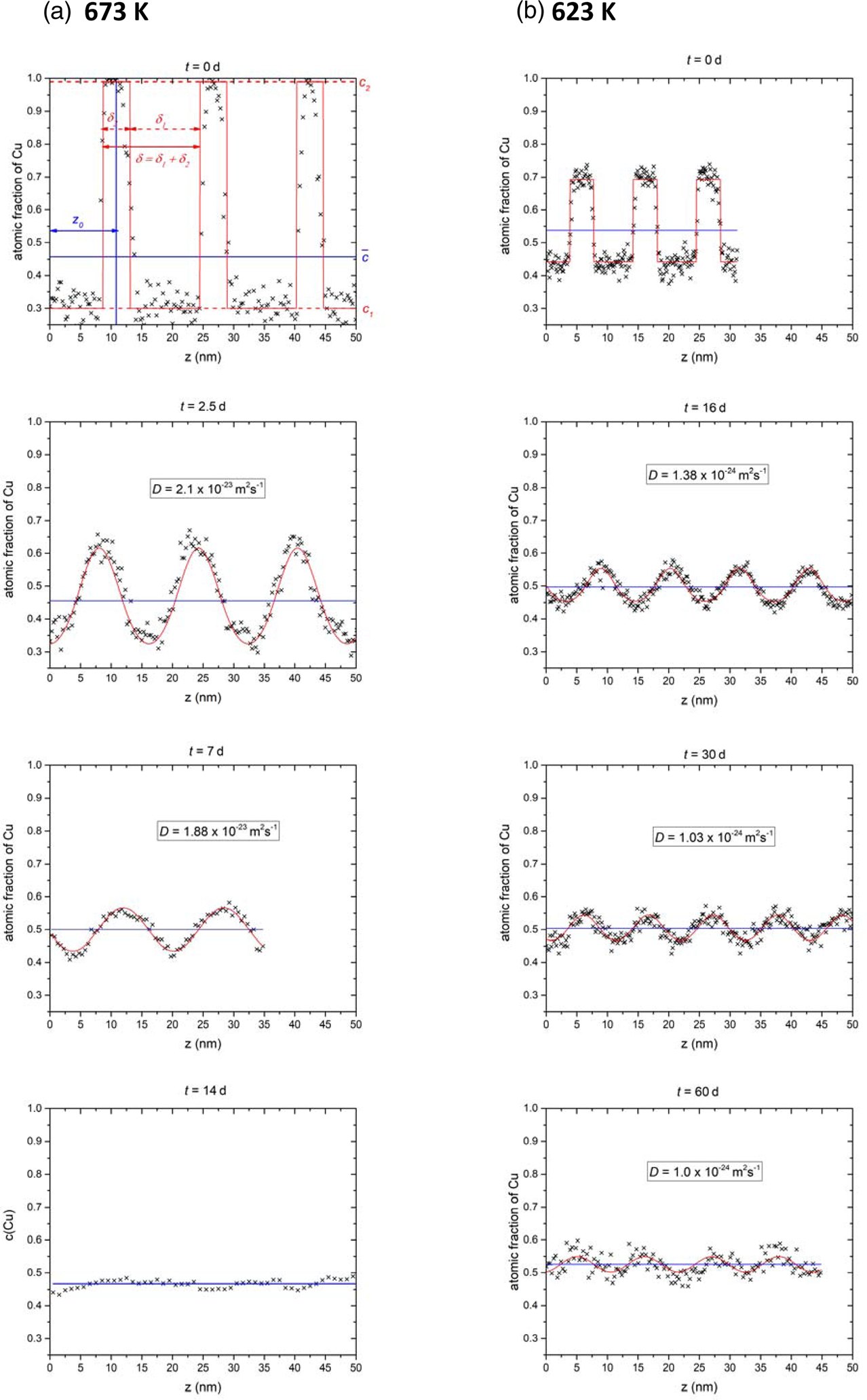
Fig. 5. Exemplary composition profiles for 673 K (a) and 623 K ((b), black crosses) at different annealing times together with the fit (red line) according to equation (1) and the average concentration (blue line).
Due to the periodic nature (Fig. 5a, top) of the layer stack, the time evolution of the composition profile is described by a Fourier series as follows:
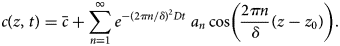 $$c( {z, \;t} ) = \bar{c} + \mathop \sum \limits_{n = 1}^\infty e^{-{( 2\pi n/\delta ) }^2Dt}\;a_n\cos \left({\displaystyle{{2\pi n} \over \delta }( {z-z_0} ) } \right).$$
The Fourier coefficients an are obtained by integrating over the full period δ = δ 1 + δ 2:
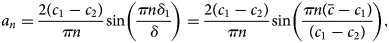 $$a_n = \displaystyle{{2( {c_1-c_2} ) } \over {\pi n}}\sin \left({\displaystyle{{\pi n\delta_1} \over \delta }} \right) = \displaystyle{{2( {c_1-c_2} ) } \over {\pi n}}\sin \left({\displaystyle{{\pi n( {\bar{c}-c_1} ) } \over {( {c_1-c_2} ) }}} \right),$$
where  $\bar{c}$ is the mean concentration, c 1 and c 2 are the initial layer concentrations, and z 0 is the spatial offset. The last identity at the right-hand side holds due to conservation of matter.
Using this equation, experimental concentration profiles for different annealing times and temperatures are fitted. With the knowledge of annealing time t and the initial layer concentration c 1 and c 2, equation (1) can be used to obtain the diffusion coefficient D, the mean concentration c̅, and the combined layer thickness δ (and offset z 0).
If the concentration in the layers evolve in time in accordance to equation (1) with a constant diffusion coefficient, the process is diffusion controlled and the system will mix completely at this temperature.
The temporal evolution of the mixing can be clearly derived from the composition profiles shown in Figure 5 for 673 K (Fig. 5a) and 623 K (Fig. 5b). The images show the experimental profiles (black crosses) and the corresponding fit (red line) with equation (1). In general, the experimental data are in good agreement, remaining differences are well explained by statistical fluctuation and possibly also some influence of reconstruction artifacts stemming from the different evaporation thresholds. The latter deviations will diminish with the annealing when the samples become chemically more homogeneous. At both temperatures, the diffusion coefficients determined by fitting remain almost constant in the course of annealing.
With increasing annealing time, the profile amplitudes are damped exponentially with time toward the average concentration (blue line). In comparison to the as-prepared state (0 d) the Cu concentration at the Ni-side (minima) of the 2.5 d and 16 d annealed samples shift only slightly (around 4%) to higher Cu concentration, whereas, on the Cu side, a large step to lower concentrations is observed. This indicates the asymmetry in the diffusivities, which is due to the concentration dependence of the diffusion coefficient. For 673 K, the profile reaches the average concentration after 14 d. Although some noise is still visible, the general trend, clearly indicates that the system is miscible at this temperature.
At 623 K, even after 60 d, a sinusoidal periodicity with 5 at% difference is still visible. However, the concentration amplitudes are continuously decreasing according to the diffusional description. Also, no plateaus of composition are formed which would be the case for phase separation. Assuming that full mixing is just not reached because of too short annealing times, the time necessary to reach phase equilibrium (less than 1 at% remaining amplitude) was determined using D from Figure 6a. It is found that at least 77 d were necessary. So, we can conclude that the system is fully miscible at this temperature.
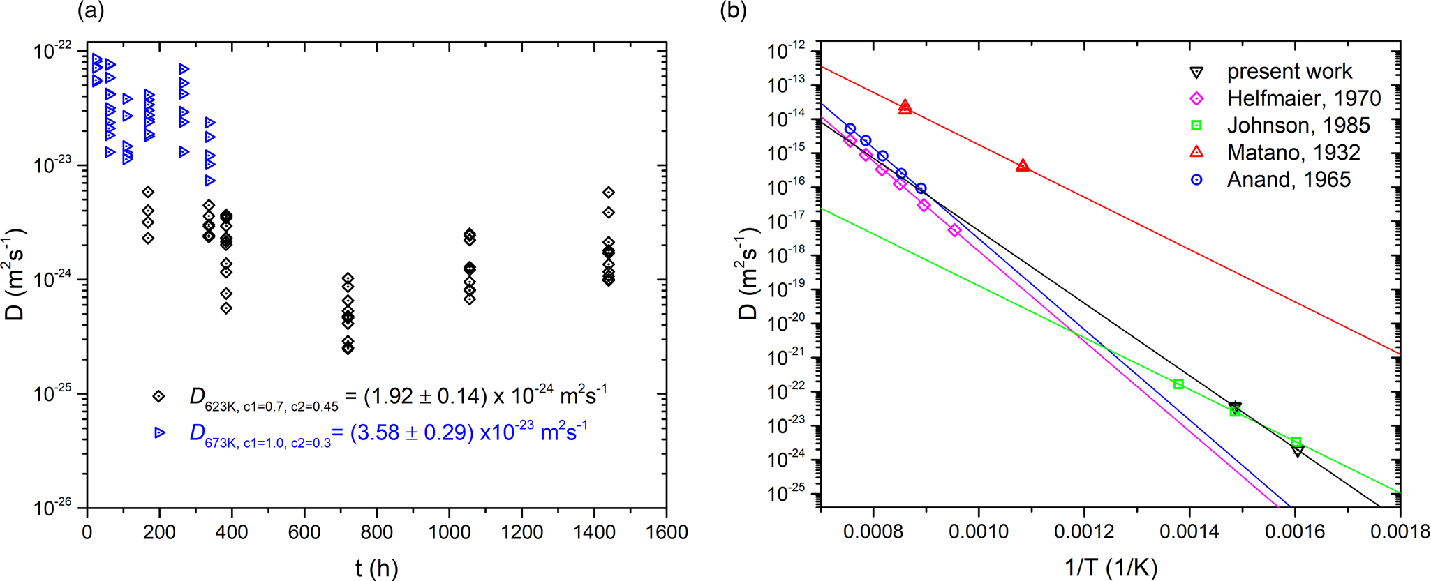
Fig. 6. (a) Diffusion coefficients D of all composition profiles measured in the present work. (b) Arrhenius plots of diffusion data of the present work in comparison to the literature. Helfmaier, Anand, and Matano studied mixing of a Cu thin films into polycrystalline Ni, whereas Johnson et al. investigated interdiffusion of CuNi thin film couples similar as in this study.
Since it is clarified that the profiles are diffusion controlled, a diffusion coefficient is determined out of the data. This knowledge is important to determine the annealing times for reaching thermodynamic equilibrium. Although several investigations were performed regarding this topic (Matano, Reference Matano1932; Anand et al., Reference Anand, Murarka and Agarwala1965; Helfmeier & Feller-Kniepmeier, Reference Helfmeier and Feller-Kniepmeier1970; Johnson et al., Reference Johnson, Bauer and Jordan1986), the resulting diffusion coefficients D exhibit a wide scattering range depending on the material structure and the used technique, in particular when extrapolated to the required low temperatures.
Therefore, we determined an effective interdiffusion coefficient D eff, valid for the nanocrystalline microstructure of this study, which is directly received from the isothermal annealing sequences by fitting with equation (1). As can be seen in equation (1), the evaluated diffusion coefficient has a quadratic dependency on the thickness. However, since the variation of layer thickness from sample to sample is determined in the fitting process, these variations are correctly treated to determine a reliable diffusion coefficient.
The results for D eff of all profiles (can be found in the Supplementary material) are plotted against the annealing time in Figure 6a. At 623 K (black diamonds), the diffusion coefficients are lower compared with 673 K (blue triangles). Although the diffusion coefficient is concentration dependent, and with time, the concentration in the layers change, the values do not show a trend with the duration of annealing. This means that a concentration dependency of D is not seen here, probably because the average concentration is reached quite fast and D corresponds closely to the concentration of 50 at%.
The coefficients of 54 profiles from 623 K and 45 profiles from 673 K were averaged and plot into an Arrhenius diagram for comparison (Fig. 6b):
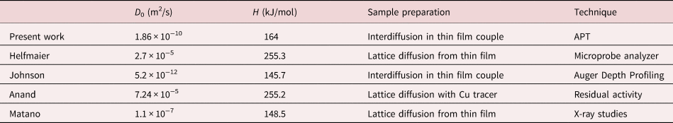
The derived characteristic parameters are: D 0 = 1.86 × 10⁻¹⁰ m2/s and H = 164 kJ/mol. In the same figure, reported literature data for chemical diffusion of Cu into Ni are shown. The characteristic parameters are presented in Table 2. Although the present study investigated the interdiffusion in a nanocrystalline microstructure (averaged on the full concentration range and possible further defect contribution), they are comparable with the diffusion of pure Cu into Ni polycrystals. The reason is that diffusion in Ni is thousand times slower [see Johnson et al. (Reference Johnson, Bauer and Jordan1986)] than diffusivity in Cu. This means that volume diffusion of Cu in Ni is the rate-determining process.
Table 2. Comparison of diffusion data found in the literature for diffusion of Cu in Ni with the effective diffusion coefficients D eff determined in this study.
Determination of Phase Boundaries
Similar to Figure 5, the composition profiles at 573 K are investigated as shown in Figure 7. In comparison to the higher temperatures, a significant difference in the mixing tendency is observed. A merging of the concentrations appears only after the first annealing time (88 d). But during longer annealing, the concentrations stay practically constant with boundary concentrations at 34.3 and 74.0 at% Cu.
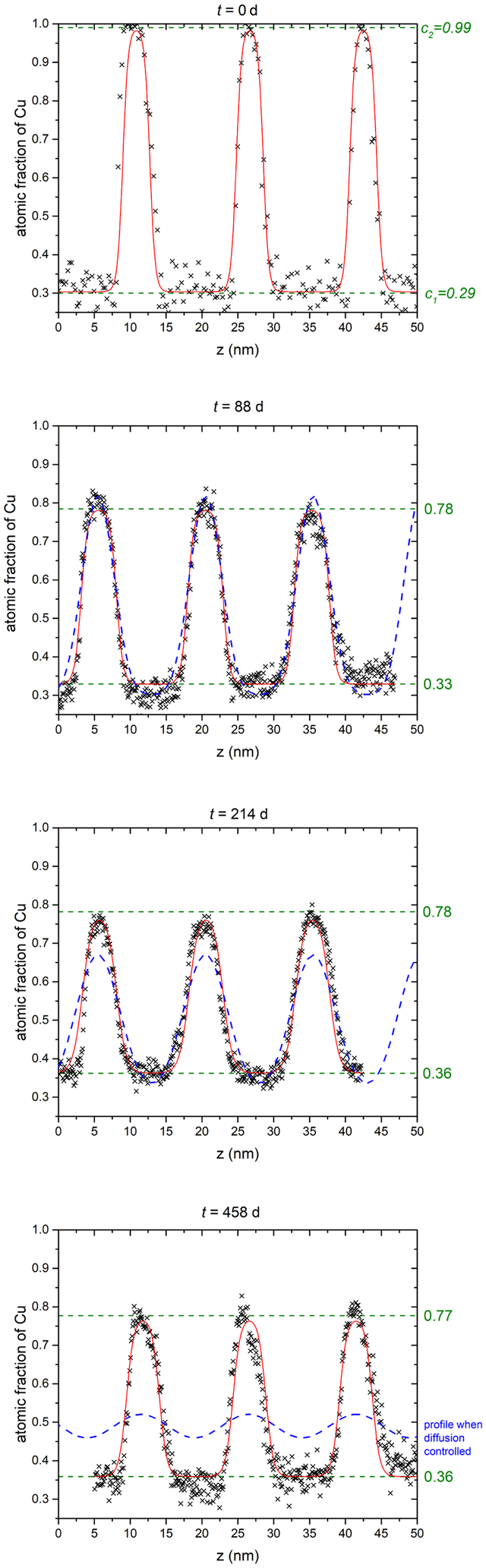
Fig. 7. Exemplary composition profiles for all annealing times of T = 573 K (black crosses) with the fit (red line) according to equation (4) and the plateau concentrations (green dashed line). The predicted profile is shown in the t = 458 d plot as a dashed blue line.
These profiles now represent two phases separated by an interface. Therefore, for quantitative evaluation, the composition profiles across the interface are modeled through sigmoids according to the Cahn–Hilliard approach (Cahn & Hilliard, Reference Cahn and Hilliard1958). Because we have periodic profiles and each period consist of two interfaces (Fig. 7), two sigmoids are required to describe a full period hi(z):
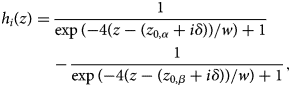 $$h_i( z ) = \displaystyle{1 \over {\exp ( {- 4( z-( z_{0, \alpha } + i\delta ) ) /w } ) + 1}}-\displaystyle{1 \over {\exp ( {- 4( z-( z_{0, \beta } + i\delta ) ) /w } ) + 1}},$$
where w is a measure of the interface width according to Cahn, δ is the period as described above, and z 0,α and z 0,β are the position of the interfaces. The full composition is given simply by superposition:
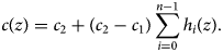 $$c( z ) = c_2 + ( {c_2-c_1} ) \mathop \sum \limits_{i = 0}^{n-1} h_i( z ). $$
With n as the number of periods and c 1 and c 2 as the compositions of the equilibrium phases.
In Figure 7, the fit is shown as a red line. The plateau concentrations (= equilibrium compositions) are marked with green dashed lines. Note that the received concentrations are slightly above the peak maxima of the fit. This is due to the narrow layer thicknesses of the Cu-rich layers which are so small that the plateau is even not reached. The plateau concentrations found for all samples are listed in the Supplementary material.
To demonstrate that really a phase separation occurred, the annealed profiles were also modeled for the diffusion-controlled case (using D from the extrapolated Arrhenius plot above). They are shown in the plots as dashed blue lines. At t = 88 d, the diffusion profile lies nearly exact on the experimental curve, indicating that this short annealing time is still diffusion-controlled. By increasing t to 214 d, a deviation of more than 10 at% at the peak maxima to the experimental curves are seen, whereas the concentration plateaus at the bottom are still fitting well. For 458 d, however, the concentration of the diffusion-controlled profile show huge discrepancy to the experimental curve and they would be way closer to the overall concentration and thus, clearly a miscibility gap is evidenced.
The observed phase boundaries clearly localize the critical temperature between 573 and 623 K. By calculating the miscibility gap from this data, T C can be determined more precisely. For that a Redlich–Kister parametrization of the Gibbs energy (Redlich & Kister, Reference Redlich and Kister1948) is used according to:
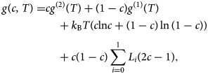 $$\eqalign{g( {c, \;T} ) = & cg^{( 2 ) }( T ) + ( {1-c} ) g^{( 1 ) }( T ) \cr & \quad + k_{\rm B}T( {c{\rm ln}c + ( {1-c} ) \ln ( {1-c} ) } ) \cr & \quad + c( {1-c} ) \mathop \sum \limits_{i = 0}^1 L_i( {2c-1} ), } $$
where the first term is the weighted average of the pure components (which is actually irrelevant for the calculation of the phase boundary), the second term is the configurational entropy, and the third term describes the deviation from ideal behavior (subregular solution).
With the free coefficients Li and c as the Ni concentration.
Using equation (5) and the double tangent method, the values for L 0 and L 1 were adapted such that the double tangent method reproduces the measured phase boundaries. They are found to be L 0 = 10.006 kJ/mol and L 1 = −0.695 kJ/mol. The complete miscibility gap can be reconstructed with the knowledge of these parameters as shown in Figure 8 as a red line. The same figure contains the experimental phase boundaries (now as Nickel concentration to compare with literature data) and the latest CALPHAD style miscibility gap (Turchanin et al., Reference Turchanin, Agraval and Abdulov2007) data by Turchanin et al. The found parameters of the miscibility gap in this study are 608 K for T C at a concentration of c(Ni) = 0.45 at% with the phase boundaries of c(Ni) = 65.7 and 26.0 at%.
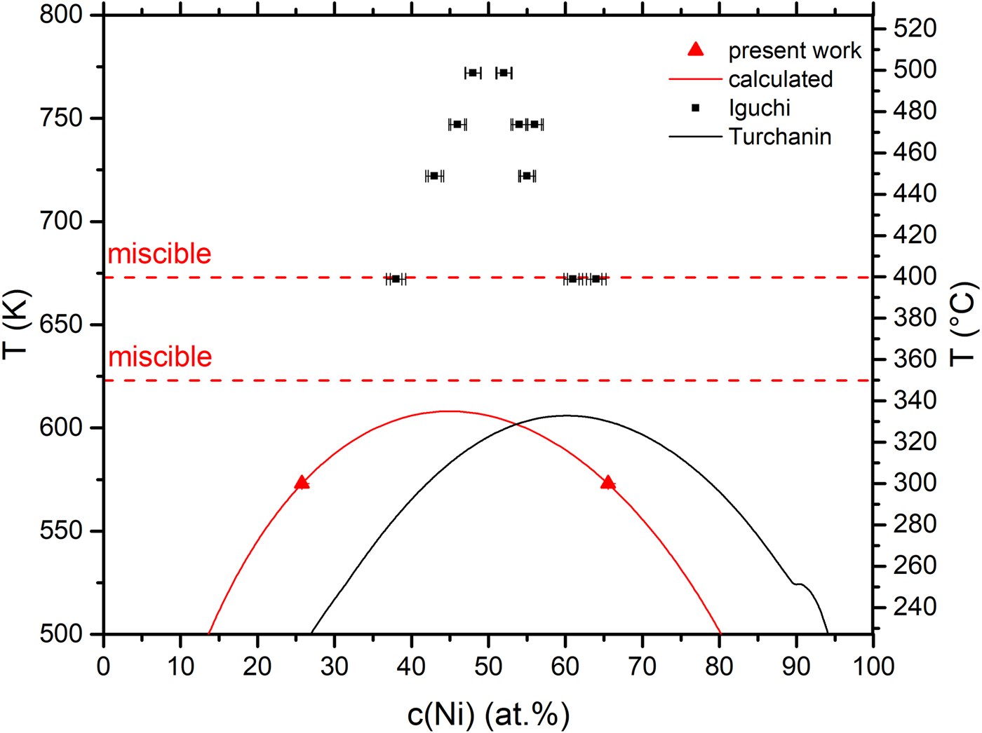
Fig. 8. (a) Measured phase boundaries at 573 K (red triangles) together with the measured miscible temperatures (horizontal, dashed red line) and the calculated miscibility gap (red line). The black line represents the latest CALPHAD miscibility gap and the black squares the one, measured experimentally by Iguchi et al. Note that here, other than in the text above, c(Ni) is used to compare the results to the literature.
Considering the critical temperature, the CALPHAD phase diagram is in well agreement to our result with a T C of 605 K. However, our experiments cannot confirm the asymmetric shift to higher Ni contents claimed by the CALPHAD approximation. Our miscibility gap is even slightly shifted to the Cu-side.
Discussion
The measured effective diffusion coefficient D eff was compared to literature values for diffusion of Cu in Ni in Figure 5b. Two high temperature measurements were made by Helfmeier and Anand with bulk Ni coated by a thin Cu film. Both studies are in good agreement to each other. However, in comparison to this study, they show a huge discrepancy. On the other hand, our data is nearly identical to previously measured diffusivity by Johnson et al., who used nearly the same temperature range for analysis on deposited Cu/Ni bilayers of 500 nm single layer thicknesses and measured the composition profiles by Scanning Auger Microprobe. The difference to the high temperature reports attributes to the sample microstructure. In the high temperature studies, single crystals or large grained polycrystals were used and so fast diffusion paths like grain boundaries or point and line defects are rare, just lattice diffusion takes place. In the low temperature studies, however, thin films were used, in which, these defects are present in high density and so, the diffusion is controlled largely by short circuit transport. In confirmation we clearly see grain boundaries. The columnar grain boundaries are regions of fast atomic transport and act as nucleation zones for diffusion controlled growth of the new (mixed) phase as shown in Figure 4. During growth, inhomogeneities are observed in bulk and grain boundary migration takes place, leaving a complete mixed phase behind. The mixing seems to be faster for specific orientations (see Fig. 4c). This observation can be explained by the system trying to reduce the nucleation energy by forming a coherent interphase with one of the grains. Consequently, the growth rates are different to both sides of interface (Porter, Reference Porter2001).
The time-dependent mixing behavior is shown via concentration profiles in Figure 6. The initial concentrations of both layers shift toward the average concentration, whereby the Cu layers make larger steps, which agrees with the faster diffusion of Ni in Cu than vice versa. The specimen is totally mixed when the concentration profiles do not oscillate anymore but a plateau at the average concentration has developed.
Comparing the time-dependent measurements of all temperatures as shown in Figure 5, such convergence to the average concentration was just observed for 673 K. At 623 K, the convergence cannot be proven directly, but since all annealing steps can be described by mixing diffusion profiles, it is practically guaranteed that also this temperature lies above miscibility gap. Furthermore, the predicted annealing time of 77 d for reaching equilibrium is not fulfilled in the experiment, where the longest duration of annealing has been 60 d. This can explain the remaining difference of 5 at% between the layer concentrations. By contrast, at 573 K (Fig. 7), stable concentration values were reached after 88 d, although the diffusion model predicts a closer merging. Thus, here the phase boundaries of the miscibility gap have been clearly reached. The phase boundaries are, therefore, localized at 34 and 74 at% for 573 K with a critical temperature at 608 K at a concentration of 45 at% of Ni. These results are compared with the broad spectrum of critical temperatures from the literature (see Table 3). Although most values are made from indirect analysis, they give a rough estimation that T C lies between 177 and 673 K. The first report on a miscibility gap in CuNi was made by Meijering et al., who analyzed the ternary NiCrCu system and found a three phase equilibrium which would just be possible, when CuNi shows phase separation. In fact, they calculated an interaction parameter that leads to a T C of 450 K, but mentioned that this is just a rough estimate.
Table 3. Literature values for critical temperature T C and boundary concentration c(Cu) in CuNi alloys.
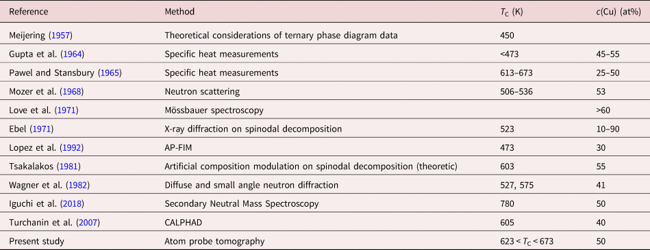
Gupta et al. measured the specific heat of CuNi at temperatures below 573 K. They measured phase boundaries with 45–55% Cu content at temperatures lower than 473 K for alloys. However, they did not make any attempt to correct their measurements. Similar calorimetric experiments were made by Pawel et al. for temperatures between 323 and 883 K and alloys of 25 and 50 at% Cu. The T C that they estimated after corrections is in good agreement to our measured data.
Mozer et al. used a neutron scattering technique on a sample with c Cu = 52.5%. A tendency of short-range clustering was found between 506 and 536 K, which is below the T C found in this work. However, Wagner et al. used the same technique and came to a similar result of 527 K like Mozer, but differentiated between a coherent and an incoherent miscibility gap. The T C of their incoherent gap has been found to be 575 K, which is very similar to our result.
X-ray measurements were made by Ebel et al. at a temperature of 523 K for different alloy concentrations. They measured spinodal decomposition ranging from 10 to 90 at%. Although we have no direct measurements at this temperature, the phase borders of the calculated miscibility gap lie in the same regime.
In Lopez et al., an alloy with 30 at% Cu content was annealed at 573 and 473 K and measured with APT. Out of the determined correlation coefficient, a clear decomposition was observed for 473 K which became weaker for 573 K, indicating that this temperature is closer to the critical temperature.
Tsalakos et al. analyzed a T C for c(Cu) = 55 at%. They measured multilayer samples of 5 nm single layer thickness with X-ray diffraction and used the “artificial modulation technique” to find out T C. In this technique, the amplitude of a composition wave is analyzed. The variation of the amplitude with annealing time is proportional to the peak intensity and thus, to the composition. By this, they came to a T C of 603 K which is in good agreement with our measurements.
By contrast, recently, another new experimental study was undertaken by Iguchi et al. using the “diffusion couple technique” for bi- and trilayer thin films of pure Cu and Ni (30–70 nm) and measuring the composition directly via depth profiling with Secondary Neutral Mass Spectrometry (SNMS; Iguchi et al., Reference Iguchi, Katona, Cserháti, Langer and Erdélyi2018). They received a T C of 780 K at a composition of 50 at% Cu, which is quite above the values reported earlier and not at least motivated us to recheck the result for layer mixing. Furthermore, their suggested shape of the solubility gap does not resemble the typical shape obtained from a (sub)regular solution model. It is in general too narrow. Our new data clearly contradict this proposition.
However, when checking the annealing times of Iguchi et al. with our diffusion model, but considering their sample depths (30 nm each) and concentrations, it is obvious that the studied annealing times of 168 h are by far not sufficient to reach equilibrium at 673 and 723 K, which should be at least 2662 and 362 h. So probably their high T C and the irregular phase boundaries are a consequence of insufficient annealing.
In the Turchanin et al. phase diagram, the proposed T C (see Fig. 8b) is in good agreement to our result. For this proposition, various experimental investigations on alloy properties (structural, electrical, and magnetic) were taken into account. In comparison to other CALPHAD approaches, Turchanin considered not just mixing enthalpies and activities from the liquid solutions, but also from solid solutions and they considered magnetic effects. Additionally, it is the only calculation, made in a self-consistent description of all data on thermodynamic properties.
While T C convincingly agrees, a huge discrepancy is seen regarding the phase boundaries between the suggested phase diagram and our experimental data. The Cu-rich phase boundary at 573 K contains around 13 at% more Ni than our results, whereas the Ni-rich phase shows a difference of 10 at%. Especially when considering the Cu-rich side (fast diffusion), the used annealing times in our experiment have to be long enough for reaching equilibrium. This can be seen also from the stable concentration values in dependence of the annealing time (Fig. 7). Only on the Ni-rich side, the slow kinetics may still allow a remaining deviation from equilibrium. Here, further demixing could shift the experimental phase boundary to Turchanin's suggestion. But the significant asymmetric positioning in the composition range appears inconsistent with our experimental findings. Further mixing experiments at temperatures above 573 K and close to T C can help clarifying this. However, the predicted annealing time at T C = 608 K is 148 d and thus quite long.
Summary
An approach for direct measurements of phase boundaries of the miscibility gap for slow diffusion couples was introduced. By using thin films of 8 nm thickness and thinner, the diffusion length could be significantly reduced. A further decrease of the annealing time is achieved by using a 30 at% pre-alloyed CuNi layer instead of pure Ni to overcome the slow diffusion on the Ni side. For evaluation, concentration profiles were used and compared to theoretical models. Isothermal annealing treatments were carried out. The results were used to determine first the effective interdiffusion coefficient D eff which is D eff = 1.86 × 10⁻¹⁰ m2/s × exp(−164 kJ/mol/RT). For 573 K, the results clearly do not follow diffusional mixing. This gives clear evidence that these limiting concentrations of c 1(Cu) = 74.0 at% and c 2(Cu) = 34.3 at% represent the real phase boundaries of the miscibility gap. With this, the miscibility gap was calculated using the Redlich–Kister parametrization of the Gibbs energy and the parameters L 0 and L 1 were determined. In comparison to the literature, the results on the critical temperature agree reasonable with the findings from Pawel and Tsakalakos and Turchanin but reject recent experimental studies by Iguchi et al.
Supplementary material
To view supplementary material for this article, please visit https://doi.org/10.1017/S1431927621012988.


 Open access