2. Problem formulation

Let us consider two identical neutrally buoyant and charge-free drops with radius $a$, viscosity $\eta _{{{d}}}$, conductivity $\sigma _{{{d}}}$ and permittivity ${\varepsilon }_{{{d}}}$ suspended in a fluid with viscosity $\eta _{{{s}}}$, conductivity $\sigma _{{{s}}}$ and permittivity ${\varepsilon }_{{{s}}}$. The mismatch in drop and suspending fluid properties is characterized by the conductivity, permittivity, and viscosity ratios

(2.1a–c)\begin{equation} R=\frac{\sigma_{{{d}}}}{\sigma_{{{s}}}},\quad S=\frac{{\varepsilon}_{{{d}}}}{{\varepsilon}_{{{s}}}},\quad \lambda=\frac{\eta_{{{d}}}}{\eta_{{{s}}}}. \end{equation}

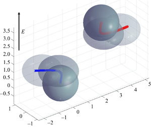
The distance between the drops’ centroids is $d$ and the angle made with the drops’ line of centres and the applied field direction is $\varTheta$. The unit separation vector between the drops is defined by the difference between the position vectors of the drops’ centres of mass $\boldsymbol {\hat {d}}=(\boldsymbol {x}_2^c-\boldsymbol {x}^c_1)/d$. The unit vector normal to the drops' line of centres and orthogonal to $\boldsymbol {\hat {d}}$ is ${\boldsymbol {\hat {t}}}$. The problem geometry is sketched in figure 1.

Figure 1. Two initially spherical identical drops with radius $a$, permittivity ${\varepsilon }_{{{d}}}$ and conductivity $\sigma _{{{d}}}$ suspended in a fluid with permittivity ${\varepsilon }_{{{s}}}$ and conductivity $\sigma _{{{s}}}$ and subjected to a uniform DC electric field $\boldsymbol {E}^\infty =E_0\boldsymbol {\hat{\boldsymbol{z}}}$. The angle between the line-of-centres vector and the field direction is $\varTheta =\arccos (\boldsymbol {\hat {z}}\boldsymbol {\cdot }\boldsymbol {\hat {d}})$.

We adopt the leaky dielectric model (Melcher & Taylor Reference Melcher and Taylor1969), which assumes creeping flow and charge-free bulk fluids acting as ohmic conductors. Albeit an approximation of the actual electrokinetic problem (Saville Reference Saville1997; Schnitzer & Yariv Reference Schnitzer and Yariv2015; Ganan-Calvo et al. Reference Ganan-Calvo, Lopez-Herrera, Rebollo-Munoz and Montanero2016, Reference Ganan-Calvo, Lopez-Herrera, Herrada, Ramos and Montanero2018; Mori & Young Reference Mori and Young2018), the leaky dielectric model has been successful in modelling many phenomena not only in poorly conducting fluids such as oils, but also aqueous electrolyte solutions such as in cell-mimicking vesicle systems (Vlahovska et al. Reference Vlahovska, Gracia, Aranda-Espinoza and Dimova2009; Vlahovska Reference Vlahovska2019). The assumption of charge-free fluids decouples the electric and hydrodynamic fields in the bulk. Accordingly,

(2.2)\begin{equation} \boldsymbol{\nabla} \boldsymbol{\cdot} \boldsymbol{T}^{{{hd}}}=\eta \nabla^2\boldsymbol{u}-\boldsymbol{\nabla} p=0,\quad \boldsymbol{\nabla}\boldsymbol{\cdot} \boldsymbol{T}^{{{el}}}=0, \end{equation}

where $T^{{{hd}}}_{ij}=-p\delta _{ij}+\eta (\partial _j u_i+\partial _i u_j)$ is the hydrodynamic stress and $\delta _{ij}$ is the Kronecker delta function; $\boldsymbol {u}$ and $p$ are the fluid velocity and pressure. The electric stress is given by the Maxwell stress tensor $T^{{{el}}}_{ij}={\varepsilon } (E_iE_j-E_kE_k\delta _{ij}/2)$. The coupling of the electric field and the fluid flow occurs at the drop interfaces $\mathcal {D}$, where the charges brought by conduction accumulate. Gauss’ law dictates that the electric field $\boldsymbol {E}$ in the electroneutral bulk fluids is solenoidal, $\boldsymbol {\nabla }\boldsymbol {\cdot } \boldsymbol {E}=0$, however, at the drop interface, the electric displacement field, ${\varepsilon } \boldsymbol {E}$, is discontinuous and its jump corresponds to the surface charge density

(2.3)\begin{equation} {\varepsilon}(E_n^{{s}}-S E_n^{{{d}}})=q, \quad \boldsymbol{x}\in \mathcal{D}, \end{equation}

where $E_n=\boldsymbol {E}\boldsymbol {\cdot }\boldsymbol {n}$, and $\boldsymbol {n}$ is the outward pointing normal vector to the drop interface. The surface charge density adjusts to satisfy the current balance

(2.4)\begin{equation} \frac{\partial q}{\partial t}+\boldsymbol{\nabla}_s\boldsymbol{\cdot}(\boldsymbol{u} q) =\sigma_{{{s}}} (E_n^{{s}}-R E_n^{{{d}}}), \quad \boldsymbol{x}\in \mathcal{D}. \end{equation}

In this study, we neglect charge relaxation and convection, thereby reducing the charge conservation equation to continuity of the electrical current across the interface as originally proposed by Taylor (Reference Taylor1966)

(2.5)\begin{equation} E_n^{{s}}=R E_n^{{{d}}}. \end{equation}

The electric field acting on the induced surface charge gives rise to an electric shear stress at the interface. The tangential stress balance yields

(2.6)\begin{equation} \left(\boldsymbol{I}-\boldsymbol{n}\boldsymbol{n}\right)\boldsymbol{\cdot} (\boldsymbol{T}^{{s}}- \boldsymbol{T}^{{{d}}})\boldsymbol{\cdot}\boldsymbol{n}+q\boldsymbol{E}_t=0, \quad \boldsymbol{x}\in \mathcal{D}, \end{equation}

where $\boldsymbol {E}_t=\boldsymbol {E}-E_n\boldsymbol {n}$ is the tangential component of the electric field, which is continuous across the interface, and $\boldsymbol {I}$ is the idemfactor. The normal stress balance is

(2.7)\begin{equation} \boldsymbol{n} \boldsymbol{\cdot}(\boldsymbol{T}^{{s}}- \boldsymbol{T}^{{{d}}})+\tfrac{1}{2}((E_n^{{{s}}})^2-S (E_n^{{{d}}})^2-(1-S)E_t^2)=\gamma(\boldsymbol{\nabla}_s\boldsymbol{\cdot} \boldsymbol{n})\boldsymbol{n}, \quad \boldsymbol{x}\in \mathcal{D}, \end{equation}

where $\gamma$ is the interfacial tension.

Henceforth, all variables are non-dimensionalized using the radius of the undeformed drops $a$, the undisturbed field strength $E_0$, a characteristic applied stress $\tau _c={\varepsilon }_{{{s}}} E_0^2$ and the properties of the suspending fluid. Accordingly, the time scale is $t_c=\eta _{{{s}}}/\tau _c$ and the velocity scale is $u_c=a \tau _c/\eta _{{{s}}}$. The ratio of the magnitude of the electric stresses and surface tension defines the electric capillary number

(2.8)\begin{equation} Ca=\frac{{\varepsilon}_{{{s}}} E_0^2 a}{\gamma}. \end{equation}

The simplification of the charge conservation equations (2.4) and (2.5) implies ${\varepsilon }^2_{{{s}}} E_0^2/(\eta _{{{s}}}\sigma _{{{s}}})\ll 1$. This condition is satisfied for the typical fluids used in experiments such as castor oil (conductivity is ${\sim }10^{-11}\ \textrm {S}\,\textrm {m}^{-1}$, viscosity is ${\sim }1\ \textrm {Pa}\,\textrm {s}$) and low field strengths $E_0\sim 10^4\ {\rm V}\ {\rm m}^{-1}$. Furthermore, the momentum diffusion time scale, $a^2\rho /\eta _{{{s}}}$, for drops of typical size $a\sim 1\ \textrm {mm}$ is much shorter than the electrohydrodynamic flow time scale $\eta _{{{s}}}/({\varepsilon }_{{{s}}} E_0^2)$, which justifies the use of the steady Stokes equation to describe the fluid flow (2.2).

3. Numerical method

We utilize the boundary integral method to solve for the flow and electric fields. Details of our three-dimensional formulation can be found in Sorgentone, Tornberg & Vlahovska (Reference Sorgentone, Tornberg and Vlahovska2019). In brief, the electric field is computed following (Baygents et al. Reference Baygents, Rivette and Stone1998; Lac & Homsy Reference Lac and Homsy2007)

(3.1)\begin{equation} \boldsymbol{E}^\infty+\sum_{j=1}^2 \int_{{\mathcal{D}}_j} \frac{\hat{\boldsymbol{x}}}{4{\rm \pi} r^3} {(\boldsymbol{E}^{{s}}-\boldsymbol{E}^{{{d}}})\boldsymbol{\cdot}\boldsymbol{n}}\,\textrm{d}S(\,\boldsymbol{y})= \begin{cases} \boldsymbol{E}^{{{d}}}(\boldsymbol{x}) & \text{if } \boldsymbol{x} \text{ inside } \mathcal{D}, \\ \tfrac{1}{2} (\boldsymbol{E}^{{{d}}}(\boldsymbol{x})+\boldsymbol{E}^{{s}}(\boldsymbol{x})) & \text{if } \boldsymbol{x} \in\mathcal{D}, \\ \boldsymbol{E}^{{s}}(\boldsymbol{x}) & \text{if } \boldsymbol{x} \text{ outside } \mathcal{D}, \end{cases} \end{equation}

where $\boldsymbol {\hat {x}}=\boldsymbol {x}-\boldsymbol {y}$ and $r=|\boldsymbol {\hat {x}}|$. The normal and tangential components of the electric field are calculated from the above equation

(3.2)\begin{equation} \left. \begin{gathered} E_n(\boldsymbol{x})=\frac{2R}{R+1}\boldsymbol{E}^\infty \boldsymbol{\cdot} \boldsymbol{n}+\frac{R-1}{R+1} \sum_{j=1}^2 \boldsymbol{n}(\boldsymbol{x})\boldsymbol{\cdot}\int_{{\mathcal{D}}_j} \frac{\boldsymbol{\hat{x}} }{2{\rm \pi} r^3} E_n(\,\boldsymbol{y})\,\textrm{d}S(\,\boldsymbol{y}),\\ \boldsymbol{E}_t(\boldsymbol{x})=\frac{\boldsymbol{E}^{{s}}+\boldsymbol{E}^{{{d}}}}{2}-\frac{1+R}{2R}E_n \boldsymbol{n}. \end{gathered} \right\} \end{equation}

For the flow field, we have developed the method for fluids of arbitrary viscosity, but for the sake of brevity here we list the equation in the case of equiviscous drops and suspending fluids. The velocity is given by

(3.3)\begin{equation} 2\boldsymbol{u}(\boldsymbol{x})=-\sum_{j=1}^2 \left( \frac{1}{4{\rm \pi}}\int_{{\mathcal{D}}_j} \left(\frac{\boldsymbol{f}(\,\boldsymbol{y})}{Ca}-\boldsymbol{f}^E(\,\boldsymbol{y})\right)\boldsymbol{\cdot} \left(\frac{\boldsymbol{I}}{r}+\frac{\boldsymbol{\hat{x}}\boldsymbol{\hat{x}}}{r^3} \right)\,\textrm{d}S(\,\boldsymbol{y})\right), \end{equation}

where $\boldsymbol {f}$ and $\boldsymbol {f}^E$ are the interfacial stresses due to surface tension and electric field

(3.4a,b)\begin{align} \boldsymbol{f}=\boldsymbol{n}\boldsymbol{\nabla}_s \boldsymbol{\cdot} \boldsymbol{n},\quad \boldsymbol{f}^E=(\boldsymbol{E}^{{s}}\boldsymbol{\cdot} \boldsymbol{n})\boldsymbol{E}^{{s}}-\tfrac{1}{2} (\boldsymbol{E}^{{s}}\boldsymbol{\cdot}\boldsymbol{E}^{{s}})\boldsymbol{n}-S((\boldsymbol{E}^{{{d}}}\boldsymbol{\cdot} \boldsymbol{n})\boldsymbol{E}^{{{d}}}-\tfrac{1}{2} (\boldsymbol{E}^{{{d}}}\boldsymbol{\cdot}\boldsymbol{E}^{{{d}}})\boldsymbol{n}). \end{align}

Drop velocity and centroid are computed from the volume averages

(3.5a,b)\begin{align} \boldsymbol{U}_j=\frac{1}{V}\int_{V_j}\boldsymbol{u}\,\textrm{d}V=\frac{1}{V}\int_{{\mathcal{D}}_j}\boldsymbol{n}\boldsymbol{\cdot}\left(\boldsymbol{u}\boldsymbol{x}\right) \,\textrm{d}S,\quad \boldsymbol{x}^c_j=\frac{1}{V}\int_{V_j}\boldsymbol{x}\, \textrm{d}V=\frac{1}{2V}\int_{{\mathcal{D}}_j}\boldsymbol{n}\left(\boldsymbol{x}\boldsymbol{\cdot} \boldsymbol{x}\right) \,\textrm{d}S. \end{align}

To solve the system of (3.2) and (3.3) we utilize the boundary integral method presented in Sorgentone et al. (Reference Sorgentone, Tornberg and Vlahovska2019). In the current study, however, we modify the time-stepper scheme to the adaptive fourth-order Runge–Kutta introduced in Kennedy & Carpenter (Reference Kennedy and Carpenter2003). All variables are expanded in spherical harmonics, which provides an accurate representation even for relatively low expansion order. In this respect, to make sure that all the geometrical quantities of interest (e.g. mean curvature) are computed with high accuracy as well, we adopt an adaptive upsampling procedure introduced by Rahimian et al. (Reference Rahimian, Veerapaneni, Zorin and Biros2015) which is based on the decay of the mean curvature spectrum and seems to work very well for this kind of simulation. When the drops are well separated from each other, the regular quadrature based on the trapezoidal rule in the longitudinal direction and on the Gauss–Legendre quadrature rule in the non-periodic direction works well. As they get closer, regular quadrature on a finer grid can still be used. Here, the density is interpolated to the finer (upsampled) grid, where the nearly singular kernel is better resolved. But at some point, a special quadrature method is needed since the quadrature error grows exponentially as we approach the surface and it is not possible to resolve the problem by grid refinement, i.e. upsampling. In Sorgentone & Tornberg (Reference Sorgentone and Tornberg2018) a numerical procedure based on interpolation first introduced by Ying, Biros & Zorin (Reference Ying, Biros and Zorin2006) is discussed and optimized to handle these complicated situations. The idea introduced in Ying et al. (Reference Ying, Biros and Zorin2006) for the nearly singular integration was to find the point $x_*$ on the surface that is closest to the target point $x_0$. Then, continuing along a line that passes through $x_*$ and $x_0$, the integral is evaluated at a number of points $x_1 ,\ldots , x_n$ further away from the surface. This can be done by regular quadrature on the standard grid or on the upsampled grid, depending on how far the target point is from the surface. The value of the integral on the surface (at $x_*$) needs to be computed by a specialized quadrature rule for singular integrals. At this point a one-dimensional Lagrangian interpolation is used to compute the value at $x_0$ by interpolating the values at $x_*$ and $x_i$, $i = 1,\ldots , N$. In Sorgentone & Tornberg (Reference Sorgentone and Tornberg2018) it has been shown how to optimize this procedure, implementing a cell list algorithm to hierarchically find the closest point on the surface and using the spherical harmonic expansion to interpolate the on-surface integral value previously obtained on the whole surface (at the grid points only) by the special quadrature for singular integrals introduced in Veerapaneni et al. (Reference Veerapaneni, Rahimian, Biros and Zorin2011) and Rahimian et al. (Reference Rahimian, Veerapaneni, Zorin and Biros2015). The accuracy of the method depends on the numerical parameters involved: the maximum distance before we need to upsample the grid for the regular quadrature (that of course will depend on the grid resolution), the upsampling rate used in the intermediate region, the number of points used for interpolation for target points in the nearest region, the distance and the distribution of these points (Sorgentone & Tornberg Reference Sorgentone and Tornberg2018). We also use the spectral reparameterization technique presented in the same paper, designed to keep the representation optimal even under strong deformations. In our work, in order to be able to run long simulations and well resolve the close interactions, we set the spherical harmonic expansion order to $p=9$, and for the nearly singular quadrature, we set the upsampling rate in the intermediate region to 4 and the number of interpolating points to 8. The viscosity contrast is $\lambda =1$. Unless otherwise explicitly stated, the electric capillary number is $Ca=0.1$.

Our numerical method was validated against the simulation results of Baygents et al. (Reference Baygents, Rivette and Stone1998) and an analytical theory for spherical drops developed by us and presented in the next section. Figure 2 shows the results for the drop steady velocity as a function of the drop centroid separation for drops aligned with the field. Figure 3 illustrates the more general case of drops initially misaligned with the field. The simulations agree very well with the theory and show a complex dynamics such as the drops line-of-centres rotating away from the applied field direction and interaction switching from attraction to repulsion. This dynamics will be explored in more detail in § 5.

Figure 2. Comparison between our fully three-dimensional simulations and the axisymmetric simulations of a drop pair aligned with the field by Baygents et al. (Reference Baygents, Rivette and Stone1998). (a) Absolute value of the radial component of the steady drop velocity as a function of separation for $Ca= 0.1$ (red dots) and 1 (blue dots) for a drop with $R=5$, $S=4$. Black dots are the data from figure 9 in Baygents et al. (Reference Baygents, Rivette and Stone1998) with $Ca=1$. Solid line is the theoretical $\boldsymbol {U}_2\boldsymbol {\cdot }\boldsymbol {\hat {d}}$ for a drop of low $Ca$ given by (4.7). The drop velocity at large separations shows the $1/d^2$ behaviour of a stresslet flow. (b) Absolute value of the steady velocity of a drop undergoing only a dielectrophoretic force, $R=S=5$, corresponding to figure 4(a) in Baygents et al. (Reference Baygents, Rivette and Stone1998). The black dots are from our fully three-dimensional code, the solid line is the dielectrophoretic velocity, (4.2), showing $1/d^4$ dependence.

Figure 3. Comparison between the simulations (black) and the analytical theory (red) for a drop pair with $R=1$, $S=3$, initial separation 3.5, initial angle between the line of centres and the applied field direction $50^{\circ }$ and $Ca=0.1$. The trajectory was computed from the relative drop velocity (4.7). Time evolution of the (a) separation, (b) angle between the line of centres and applied field direction, (c) radial component of the relative velocity $\boldsymbol {U}\boldsymbol {\cdot }\boldsymbol {\hat {d}}$ and (d) tangential component of the relative velocity $\boldsymbol {U}\boldsymbol {\cdot }{\boldsymbol {\hat {t}}}$.

4. Theory: far-field interactions

To gain more physical insight, it is instructive to analyse the interaction of two widely separated spherical drops. In this case, the drops can be approximated as point dipoles. The disturbance field $\boldsymbol {E}_1$ of the drop dipole $\boldsymbol {P}_1$ induces a dielectrophoretic (DEP) force on the dipole $\boldsymbol {P}_2$ located at $\boldsymbol {x}^c_2=d\boldsymbol {\hat {d}}$, given by $\boldsymbol {F}(d)=(\boldsymbol {P}_2\boldsymbol {\cdot } \boldsymbol {\nabla } \boldsymbol {E}_1)|_{r=d}$

(4.1)\begin{equation} \boldsymbol{F}(d)=\boldsymbol{P}_1\boldsymbol{P}_2:\boldsymbol{\nabla} \left.\left(\frac{\boldsymbol{I}}{r^3}-3\frac{\boldsymbol{x}\boldsymbol{x}}{r^5}\right)\right|_{r=d},\quad \boldsymbol{P}_1=\boldsymbol{P}_2=\frac{R-1}{R+2}\boldsymbol{E}^\infty. \end{equation}

The drop velocity under the action of this force can be estimated from Stokes’ law, $\boldsymbol {U}^{{{dep}}}_2=-\boldsymbol {U}^{{{dep}}}_1=\boldsymbol {F} /\zeta$, where $\zeta$ is the friction coefficient, $\zeta =2{\rm \pi} (3\lambda +2)/(\lambda +1)$

(4.2)\begin{equation} \boldsymbol{U}_2^{{{dep}}}=\frac{\beta_D}{r^4}\frac{3(1+{\lambda})}{2+3{\lambda}}[(1-3\cos^2\varTheta)\boldsymbol{\hat{d}}-\sin\left(2\varTheta\right){\boldsymbol{\hat{t}}}],\quad \beta_D= \left(\frac{R-1}{R+2}\right)^2. \end{equation}

The relative DEP velocity, $\boldsymbol {U}^{{{dep}}}=\boldsymbol {U}^{{{dep}}}_2-\boldsymbol {U}^{{{dep}}}_1$, depends on the angle $\varTheta =\arccos (\boldsymbol {\hat {d}}\boldsymbol {\cdot }\boldsymbol {\hat {z}} )$ between the direction of the external field and the line joining the centres of the two drops. Drops attract, i.e. $\boldsymbol {U}^{{{dep}}}\boldsymbol {\cdot }\boldsymbol {\hat {d}}<0$, if $\varTheta <\varTheta _c=\arccos ({1}/{\sqrt {3}})\approx 54.7^{\circ }$, e.g. when the drops are lined up with the field, and repulse if $\varTheta >\varTheta _c$, e.g. if the line of centres of the two drops is perpendicular to the field. The DEP interaction also causes drops to align with the field, since the tangential component of the relative velocity is always negative.

The electrohydrodynamic (EHD) flow about an isolated, spherical drop in an applied uniform electric field is a combination of a stresslet and a quadrupole (see appendix A for the flow evolution upon application of the electric field). At steady state,

(4.3)\begin{equation} \boldsymbol{u} = \frac{9}{10}\frac{S-R}{(2+R)^2(\lambda+1)}\boldsymbol{E^\infty E^\infty} : \left[\left(\frac{\boldsymbol{I}}{r^3}-3\frac{\boldsymbol{xx}}{r^5}\right)\boldsymbol{x} + \frac{1}{3}\boldsymbol{\nabla}\left(\frac{\boldsymbol{I}}{r^3}-3\frac{\boldsymbol{xx}}{r^5}\right) \right]. \end{equation}

At the surface of the drop,

(4.4)\begin{equation} \boldsymbol{u}\left(r=1\right)=\beta_T\sin(2\theta){\boldsymbol{\hat{\theta}}},\quad \beta_T=\frac{9}{10}\frac{R-S}{\left(1+\lambda\right)\left(R+2\right)^2}. \end{equation}

If $R/S<1$, the surface flow is from pole to equator, i.e. fluid is drawn in at the poles and pushed away from the drop at the equator. The flow direction is reversed for ${R/S>1}$. A second drop moves in response to the EHD flow (4.3). The drop translational velocity is found from Faxen's law (Kim & Karrila Reference Kim and Karrila1991)

(4.5)\begin{equation} {\boldsymbol{U}}^{{{ehd}}}_{2} = \left(1 + \frac{\lambda}{2(3\lambda+2)}\nabla^2\right)\boldsymbol{u}|_{\boldsymbol{x}=d\boldsymbol{\hat{d}}}. \end{equation}

Inserting (4.3) in the above equation leads to

(4.6)\begin{align} {\boldsymbol{U}}^{{{ehd}}}_{2} &= \beta_T\left(\frac{1}{ d^2}-\frac{2}{d^4}\left(\frac{1+3{\lambda}}{2+3{\lambda}}\right)\right)(-1+3 \cos^2\varTheta)\boldsymbol{\hat{d}}\nonumber\\ &\quad -\frac{2\beta_T}{d^4}\left(\frac{1+3{\lambda}}{2+3{\lambda}}\right)\sin(2\varTheta){\boldsymbol{\hat{t}}}+O(d^{-5}). \end{align}

The radial component of the EHD velocity, and thus the sign of the EHD interaction (attraction or repulsion), changes sign at the same angle as the DEP interaction, $\varTheta _c=54.7$. If $R/S<1$, the EHD flow is attractive when drops are aligned with the applied field and repulsive when the line of centres is perpendicular to the field direction. The interaction is reversed for $R/S>1$. Notably, unlike the DEP interaction which always drives the drops to align with the applied field direction, the EHD can cause the drops’ line of centres to rotate away from the direction of the applied field if $\beta _T<0$, i.e. $R/S<1$.

Combining the EHD and the DEP velocities yields the relative drop velocity. Since the drops studied here are identical, drop motions are reciprocal. Therefore, the relative drop velocity $\boldsymbol {U}=\boldsymbol {U}_2-\boldsymbol {U}_1=2\boldsymbol {U}_2$

(4.7)\begin{align} \boldsymbol{U}=\frac{2\beta_T}{ d^2}(-1+3 \cos^2\varTheta)\boldsymbol{\hat{d}}-\varPhi(R, S, {\lambda})\frac{4}{d^4}((-1+3 \cos^2\varTheta)\boldsymbol{\hat{d}}+\sin(2\varTheta){\boldsymbol{\hat{t}}})+O(d^{-5}), \end{align}

where

(4.8)\begin{equation} \varPhi=\frac{1+3{\lambda}}{2+3{\lambda}}\left(\beta_T+3\beta_D\frac{1+\lambda}{1+3\lambda}\right). \end{equation}

The discriminant ${\varPhi }$ quantifies the drop pair alignment with the field and the interplay of EHD and DEP interactions in drop attraction or repulsion. The line of centres between two drops with $\varPhi >0$ rotates towards a parallel orientation with respect to the applied electric field, since $\dot \varTheta =\boldsymbol {U}\boldsymbol {\cdot } {\boldsymbol {\hat {t}}}\sim -\varPhi$. However, in the case of $\varPhi < 0$ (which occurs only for $R/S<1$ drops), the line of centres between the drops rotates towards a perpendicular orientation with respect to the applied electric field. Figure 4(a) summarizes the regimes of alignment and deformation.

Figure 4. (a) Phase diagram of drop deformations and alignment with the field for different viscosity ratios. The solid lines correspond to $\varPhi ({\lambda }, R, S)=0$ given by (4.8). In the shaded regions, the line of centres of the two drops rotates away from the applied field direction $\varPhi <0$. The dashed line corresponds to the Taylor discriminating function (A3); in the parameter space above it, drop deformation is oblate. (b) Critical separation above which EHD dominates the interactions for ${\lambda }=1$ and $S=0.1$ (blue), $S=1$ (black) and $S=10$ (red).

The relative radial motion of the two drops at a given configuration depends on $\varPhi$ and $\beta _T$, where $\beta _T \boldsymbol {\hat {z}}\boldsymbol {\hat {z}}$ is the strength of the far-field EHD stresslet flow

(4.9)\begin{equation} \boldsymbol{u}_s\left(\boldsymbol{x}\right)=\beta_T(-1+3 \cos^2 \theta)\frac{\boldsymbol{x}}{r^3}. \end{equation}

There is a critical separation $d_c$ corresponding to $\boldsymbol {U}_2(d_c)\boldsymbol {\cdot }\boldsymbol {\hat {d}}=0$, which yields $d_c^2=2\varPhi /\beta _T$. For $\varPhi > 0$ and $R/S<1$ ($\beta _T<0)$, $d_c$ does not exist and EHD and DEP interactions are cooperative and act radially in the same direction (note that a system with $\varPhi <0$ and $R/S>1$ cannot exist). For $\varPhi > 0$ and $R/S>1$ or $\varPhi <0$ and $R/S<1$, there is competition between EHD and DEP, with the quadrupolar DEP winning out closer to the drops and the EHD taking over via the stresslet flow in the far field. The fact that depending on separation drops may attract or repel in the case of antagonistic EHD and DEP interactions has been discussed previously by Baygents et al. (Reference Baygents, Rivette and Stone1998) and Zabarankin (Reference Zabarankin2020). Note that for drops with $R/S<1$, EHD effectively dominates DEP at all separations since $d_c$ is smaller than 2, which is the minimum separation of spherical drops. Figure 4(b) illustrates the dependence of the critical separation $d_c$ for three typical cases. If $S=10$, $d_c$ is always less than 2, the minimum separation between two spheres, and accordingly the interactions are dominated by the EHD flow. For $S=1$, $d_c$ does not exist below $R=0.7$. In the case $S=0.1$, $\varPhi >0$ for all values of $R$ and thus $R/S<1$ is always dominated by EHD, while in the case $R/S>1$ the DEP attraction could be stronger than the EHD for quite large separations, e.g. for $R/S=1.1$ or $R/S\gg 1$ $d_c > 10$. The DEP dominates in these cases because the EHD is very weak, in the first case because $(R-S)\sim 0$ and in the second case because the EHD flow decreases with conductivity ratio as ${\sim }1/R$.