


1. Introduction
We investigate the incompressible flow of a Herschel–Bulkley viscoplastic fluid between two rigid, semi-infinite plates, hinged at the origin and rotating towards one another with angular velocity,  $\varOmega$ (see figure 1a), thus extending the classical problem of viscous Newtonian fluid flow in this configuration (see, for example, Moffatt (Reference Moffatt1964)). Recent studies of viscoplastic fluids in converging and recirculating corner flows have demonstrated how the existence of a yield-stress changes the structure of the Newtonian solutions significantly, leading to the occurrence of rigid unyielded regions of fluid, or ‘plugs’, and the development of viscoplastic boundary layers when the dimensionless yield-stress is large (Taylor-West & Hogg Reference Taylor-West and Hogg2021, Reference Taylor-West and Hogg2022). In both of these previous studies, the magnitude of the strain rate varies with the distance from the vertex, resulting in viscously and yield-stress dominated behaviour in different regions of the wedge. In contrast, it will be shown that the flow driven by hinged plates is self-similar, with the dimensionless strain rate and deviatoric stresses varying only with the polar angle. This flow configuration has application to coating (Davard & Dupuis Reference Davard and Dupuis2000), lubrication (for example in the biomechanics of synovial joints (Hou et al. Reference Hou, Mow, Lai and Holmes1992)) and extrusion flows of viscoplastic fluid (Ahuja, Luisi & Potanin Reference Ahuja, Luisi and Potanin2018). In sensory evaluation of foods, Chen (Reference Chen1993) suggests that squeeze flow in a wedge more accurately models the flow between the tongue and roof of mouth than the flow between parallel plates, which has been used as a model to predict oral sensory response (for example, Demartine & Cussler (Reference Demartine and Cussler1975) and Elejalde & Kokini (Reference Elejalde and Kokini1992)). In addition, albeit with different boundary conditions, the flow in a closing wedge could be used to understand the local flow near a moving contact line in a drop of yield-stress fluid (see, for example, Jalaal, Stoeber & Balmforth (Reference Jalaal, Stoeber and Balmforth2021)). Beyond its direct relevance to applications, the flow configuration under consideration in this study also offers a rare example of a quasianalytical solution for non-Newtonian, non-parallel flow. As such it is a useful problem for bench-marking computational codes and for determining the validity of constitutive models beyond simple-shear flows in which they are typically defined and experimentally determined.

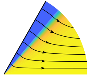
Figure 1. (a) Schematic of problem geometry. Only half of the geometry is shown, with the other half given by symmetry in  $\theta =0$. The shaded region indicates unyielded material. (b) Strain-rate (colour-plot) and streamlines (black) from numerical integration as described in § 3, with
  $\alpha =60^{\circ }$,
  $Bi=1000$ and
  $N=1$. The solid blue region shows the unyielded plug.
The flow between rotating hinged plates has been studied for a number of different non-Newtonian constitutive laws. Phan-Thien (Reference Phan-Thien1984) studied the case of a viscoelastic fluid, showing that exact similarity solutions exist for a general viscoelastic constitutive law, and analysing in detail the time evolution for the specific examples of the Oldroyd-B and Phan-Thien and Tanner (PTT) models, with a prescribed exponential closing rate of the hinged plates. They showed that the velocity fields do not deviate significantly from the Newtonian solution, but that viscoelasticity can have a significant impact on the evolution of the stresses in the wedge, with the Oldroyd-B model, in particular, predicting unbounded extensional stresses above a critical Weissenberg number (the ratio of typical elastic and viscous stresses), while stresses in the PTT model remain bounded but can become oscillatory. Phan-Thien & Zheng (Reference Phan-Thien and Zheng1991) further explored the existence of this critical Weissenberg number, by focussing on the steady-state solution at a given hinge half-angle (of  ${\rm \pi} /4$) and showing that, for an Oldroyd-B fluid, the critical Weissenberg number corresponds to a limiting point above which the steady-state solution ceases to exist. Chen (Reference Chen1993) studied the problem for a power-law fluid, using an assumed approximate form for the radial velocity field in the cases of slip and no-slip at the walls, with the aim of providing more easily calculated solutions than the exact similarity solutions derived by Phan-Thien (Reference Phan-Thien1984). Wilson (Reference Wilson1993) investigated the flow of a biviscosity fluid in a closing wedge of half-angle less than
  ${\rm \pi} /4$. Under this rheological model the fluid is assumed to be Newtonian with relatively high viscosity up to an imposed transitional shear stress (or equivalently a transitional strain rate) and then exhibits a Bingham-like constitutive law for high shear stresses and strain rates; by construction the constitutive law is continuous. In the limit where the ratio of the viscosities above and below the transitional strain rate vanishes, the Bingham law is retrieved. Often with this model, a ‘yield surface’ is defined as a location at which the flow attains the transitional strain rate and changes its rheological model from Newtonian to Bingham-like. Evidently this surface does not demark the boundary of an unyielded rigid plastic region, since deformation is still permitted, albeit with a potentially high viscosity. Wilson (Reference Wilson1993) determined the existence of the ‘yield surface’ and its dependence upon the dimensionless transitional shear stress and the ratio of the viscosities. He showed that the material close to the symmetry line of the wedge could be ‘unyielded’ (i.e. its strain rate falls below the transitional value), but that this region vanished when the viscosity ratio became sufficiently small for any fixed dimensionless transitional shear stress, in which case the entire fluid was ‘yielded’. As we demonstrate below (see §§ 3 and 4), for wedge angles less than
  ${\rm \pi} /4$, the fluid is indeed yielded throughout, and is plastically dominated and only weakly yielded when the dimensionless yield stress is large. It is also possible to explore the dynamical behaviour under other regularised rheologies within the wedge. For example, Al Khatib (Reference Al Khatib2006) considered the problem for a regularised version of the Herschel–Bulkley constitutive law, deriving the governing similarity equations for the time evolution of the flow under a prescribed exponential closing rate, utilising the Papanastasiou regularisation. They found that the radial velocity distribution was very close to the Newtonian solution for the range of parameters explored, and showed how the pressure load on the plates varied with time and depended on the shear thinning and yield stress of the fluid. They also considered the existence of unyielded regions in the wedge and found that no such region exists, however, their analysis is for just a single choice of the hinge angle and constitutive parameters and, moreover, the regularisation of the constitutive law precludes the occurrence of any true plugs (as for the biviscosity model).
Compression between rotating hinged plates has also been widely studied for a plastic material, under a range of different constitutive laws (Alexandrov & Lyamina Reference Alexandrov and Lyamina2003; Alexandrov & Jeng Reference Alexandrov and Jeng2009; Alexandrov, Pirumov & Chesnikova Reference Alexandrov, Pirumov and Chesnikova2009; Alexandrov & Miszuris Reference Alexandrov and Miszuris2015). A distinguished feature of the rigid plastic problem is the existence of unyielded regions in rigid body rotation adjacent to the rotating plates, for sufficiently large wedge angles. Of particular relevance to the current paper are the studies for a Bingham viscoplastic (Alexandrov & Jeng Reference Alexandrov and Jeng2009), and for a viscoplastic with a saturation stress which the magnitude of the deviatoric stress approaches as the strain-rate tends to infinity (Alexandrov & Miszuris Reference Alexandrov and Miszuris2015). In the former, Alexandrov & Jeng (Reference Alexandrov and Jeng2009) show that the deviatoric stresses are functions of polar angle only, and hence derive governing ordinary differential equations (ODEs) for the stress and velocity fields in the domain. Their results do not exhibit plug formation or boundary layers in part due to the focus on relatively small yield stresses and angles between the plates. In the latter, Alexandrov & Miszuris (Reference Alexandrov and Miszuris2015) show that a rigid zone can occur for wedge angles above some critical value but, in the absence of a specific constitutive law, do not calculate this angle or evaluate how it depends on the non-dimensional yield stress. The existence of typical viscoplastic boundary layers in this case is precluded by the saturation stress which results in plastic behaviour when the shear-rate is large. Herein, we revisit the solution of Alexandrov & Jeng (Reference Alexandrov and Jeng2009) for the case of a Bingham fluid, which we generalise to the Herschel–Bulkley constitutive law, demonstrating that the self-similar solution does in fact include the existence of unyielded regions for sufficiently large angles between the plates, and elucidating the boundary-layer structure that emerges in the regime of large non-dimensional yield-stress.
We assume the constitutive law of a Herschel–Bulkley fluid, relating the deviatoric stress tensor,  $\boldsymbol {\tau }$, to the strain-rate tensor,
  $\boldsymbol {\dot {\gamma }}=\boldsymbol {\nabla }\boldsymbol {u}+\boldsymbol {\nabla }\boldsymbol {u}^{\rm T}$, via
 \begin{equation} \boldsymbol{\tau}=\left(K\dot{\gamma}^{N-1}+\frac{\tau_Y}{\dot{\gamma}}\right)\boldsymbol{\dot{\gamma}} \quad \text{when } \tau>\tau_Y, \quad \dot{\gamma}=0 \text{ otherwise}, \end{equation}
where  $K$ is the consistency,
  $N$ is the flow index,
  $\tau _Y$ is the yield-stress and
  $\tau \equiv (\tau _{ij}\tau _{ij}/2)^{1/2}$ and
  $\dot {\gamma }\equiv (\dot {\gamma }_{ij}\dot {\gamma }_{ij}/2)^{1/2}$ are the second invariants of the deviatoric stress and strain-rate tensors, respectively. This constitutive law reduces to the Bingham model for
  $N=1$ and
  $K=\mu$, the viscosity. We adopt polar coordinates,
  $(r,\theta )$, centred on the hinge and with
  $\theta$ measured from the line of symmetry between the two plates (see figure 1). We denote the components of the velocity as
  $\boldsymbol {u}=(u,v)$. Assuming
  $\rho \varOmega ^{2-N} r^2/K\ll 1$ (where
  $\rho$ denotes the density) in the region of interest, we can neglect inertia and search for a quasistatic solution. In this case, the system of equations is given by
 $$\begin{gather} \frac{1}{r}\frac{\partial}{\partial r}\left(ru\right)+\frac{1}{r}\frac{\partial v}{\partial \theta}=0, \end{gather}$$
 $$\begin{gather}\frac{\partial p}{\partial r}=\frac{\partial \tau_{rr}}{\partial r}+\frac{1}{r}\frac{\partial \tau_{r\theta}}{\partial \theta}+\frac{2}{r}\tau_{rr}, \end{gather}$$
 $$\begin{gather}\frac{1}{r}\frac{\partial p}{\partial \theta}=\frac{\partial \tau_{r\theta}}{\partial r}-\frac{1}{r}\frac{\partial \tau_{rr}}{\partial \theta}+\frac{2}{r}\tau_{r\theta}, \end{gather}$$
representing incompressibility, and the balance of momentum in the radial and azimuthal directions, respectively. The boundary conditions arise from symmetry at  $\theta =0$ and no-slip at the rigid wall, and are given by
 \begin{equation} v=\frac{\partial u}{\partial \theta}=0 \ \text{at}\ \theta=0, \quad \text{and}\quad \left(u, v\right)=\left(0, -\varOmega r\right) \ \text{at}\ \theta=\alpha, \end{equation}
when the rigid plates are at  $\theta =\pm \alpha$.
We note that, in the absence of a length scale in the problem, the only velocity scale is  $\varOmega r$ and so we write
 \begin{equation} (u,v)=\frac{\varOmega r}{2}\left(f'(\theta),-2f(\theta)\right),\end{equation}
where  $f(\theta )$ is a function to be determined, and then incompressibility is automatically satisfied; the stream function is therefore given by
  $\varPsi =\varOmega r^2f(\theta )/2$. We further scale strain-rates by
  $\varOmega /2$, and pressure and stresses by the viscous stress scale
  $K (\varOmega /2)^N$. Having done so, the governing equations for the dimensionless variables are unchanged but the constitutive law becomes
 \begin{equation} \boldsymbol{\tau}=\left(\dot{\gamma}^{N-1}+\frac{Bi}{\dot{\gamma}}\right)\boldsymbol{\dot{\gamma}} \ \text{when } \tau>Bi, \quad \dot{\gamma}=0\ \text{ otherwise}, \end{equation}
where the dimensionless parameter,  $Bi=2^N\tau _Y/(K\varOmega ^N)$, is the Bingham number, representing the ratio of the yield-stress to a typical viscous stress. Further, the boundary conditions become
  $f=f''=0 \text { at } \theta =0, \text { and } f=1, f'=0 \text { at } \theta =\alpha$, representing assumed symmetry at
  $\theta =0$ and no slip at
  $\theta =\alpha$.
As shown by Alexandrov & Jeng (Reference Alexandrov and Jeng2009), under the self-similar ansatz (1.6), the governing equations reduce to ODEs. By careful analysis of these governing differential equations we will show that a rigid zone adjacent to the boundary, in which the fluid is in solid body rotation, does exist for angles above a critical angle,  $\alpha \geq \alpha _c$ (with
  $\alpha _c\geq {\rm \pi}/4$), and demonstrate how this critical angle depends on the Bingham number, in particular reducing asymptotically to
  ${\rm \pi} /4$ in the plastic limit
  $Bi\to \infty$. We will also show that viscoplastic boundary layers occur when
  $Bi\gg 1$, demonstrating the dependence of the width of these layers on the Bingham number.
The theory of viscoplastic boundary layers, in which shear becomes concentrated in a thin layer, was first developed by Oldroyd (Reference Oldroyd1947), who identified a distinguished limit in which viscous and plastic stresses both enter the leading-order balance of momentum in the boundary layer. For a Bingham fluid, this regime occurs for dimensionless boundary layer widths of order  $Bi^{-1/3}$. Later, Piau (Reference Piau2002) proposed an alternative boundary layer scaling, of order
  $Bi^{-1/2}$, for which viscous stresses are dominant in the boundary layer. These theories were generalised and put on a rigorous asymptotic footing by Balmforth et al. (Reference Balmforth, Craster, Hewitt, Hormozi and Maleki2017). Such boundary layers have also been observed in laboratory experiments, in the penetration of a rigid plate into a bath of viscoplastic fluid (Boujlel et al. Reference Boujlel, Maillard, Lindner, Ovarlez, Chateau and Coussot2012), and the injection of viscoplastic fluid into a bath of the same fluid (Chevalier et al. Reference Chevalier, Rodts, Chateau, Boujlel, Maillard and Coussot2013). Chevalier et al. (Reference Chevalier, Rodts, Chateau, Boujlel, Maillard and Coussot2013) associates the existence of these boundary layers with the flow becoming ‘frustrated’ when the yield stress character locks the fluid in place, while boundary conditions necessitate motion of the fluid. Thus, when the yield stress is large, boundary layers occur to break this frustration, by allowing for the motion of the boundaries while the bulk of the fluid remains at the yield stress. For the current problem we will show that boundary layers of this kind form at the rigid boundaries when the Bingham number is large and the wedge half-angle is below
  ${\rm \pi} /4$ (
 $\alpha _c-\alpha =O(1)$). Conversely, for
  $\alpha$ beyond this regime the flow can satisfy the velocity boundary conditions without requiring a region of high strain rate, and so the strain rates remain
  $O(1)$, and the fluid remains at the yield stress to leading order throughout the wedge. In accord with previous studies, the dimensionless width of the boundary layers scales with the Bingham number via
  $Bi^{-1/(N+1)}$, reducing to the anticipated
  $Bi^{-1/2}$ scaling for Bingham fluids. We note that Wilson's (Reference Wilson1993) analysis of the biviscosity model in wedges with
  $\alpha <{\rm \pi} /4$ in the regime of relatively high transitional shear stress also features boundary layers attached to the wedge boundaries. They scale in accord with the Bingham case of
  $N=1$ with the dimensionless width being proportional to
  $Bi^{-1/2}$. It will be shown in § 4.1 that our approach circumvents some of the difficulties of Wilson's (Reference Wilson1993) analysis by a different choice of independent variable (see § 2) and explicitly matches between a plastically dominated region in the bulk and viscously deforming region adjacent to the wedge boundaries. This allows extension to both Herschel–Bulkley rheology and to wider wedge angles
  $(\alpha >{\rm \pi} /4)$ for which rigid plug regions exist adjacent to the wedge boundaries.
We first derive the similarity equations, extending the methodology of Alexandrov & Jeng (Reference Alexandrov and Jeng2009) in § 2, then detail the numerical integration of these ODEs in § 3 and set out the boundary layer analysis in § 4. In § 5 we carry out full numerical simulations of the problem, to show how the similarity solution is embedded in the full simulations, before briefly concluding in § 6. There is also one Appendix in which we detail how the results reduce to the Newtonian solution when  $Bi\ll 1$ with
  $N=1$, and determine the asymptotic dependence of a thin unyielded region near the plates when
  $\alpha ={\rm \pi} /2$ in this regime.
2. Similarity equations
Given the assumed form of the velocity (1.6), the strain-rate components and magnitude of the strain rate are given in dimensionless form by
 \begin{equation} \dot{\gamma}_{rr}=2f'(\theta), \quad \dot{\gamma}_{r\theta}=f''(\theta), \quad \dot{\gamma}=\sqrt{f''^2+4f'^2}, \end{equation}
where a prime denotes differentiation with respect to  $\theta$. Importantly these are independent of radial distance from the vertex and this underpins the solution that we develop in what follows. An immediate consequence is that the components of the stress tensor are also functions of only the polar angle and we can write
 \begin{equation} \begin{pmatrix} \tau_{rr}\left(\theta\right) \\ \tau_{r\theta}\left(\theta\right) \end{pmatrix}=k(\theta)\begin{pmatrix} \cos2\psi \\ -\sin2\psi \end{pmatrix}, \end{equation}
where  $\psi =\psi (\theta )$ is a variable representing the orientation of the deviatoric stress tensor and the magnitude of the deviatoric stress,
  $k(\theta )$, is given by
 \begin{equation} k(\theta)=\left(f''^2+4f'^2\right)^{N/2}+Bi, \end{equation}
wherever the fluid is yielded. By symmetry  $\psi =0$ at
  $\theta =0$ and, since
  $u$ vanishes on the wall,
  $\tau _{rr}=0$ and so
  $\psi ={\rm \pi} /4$ at
  $\theta =\alpha$. Furthermore, if there is a rigid region for
  $\theta \geq \alpha _c$ then
  $\psi ={\rm \pi} /4$ and
  $f''=0$ at
  $\theta =\alpha _c$ (since the strain rate must vanish at the unyielded plug). The azimuthal pressure gradient is found to be independent of
  $r$ and thus the pressure takes the form
 \begin{equation} p=2ABi\log r+g(\theta), \end{equation}
where  $A$ is a constant, and so the balance of radial and angular momentum reduce to
 $$\begin{gather} 2Bi A ={-}\frac{\text{d}k}{\text{d}\theta}\sin2\psi + 2k\cos2\psi\left(1-\frac{\text{d}{\psi}}{\text{d}\theta}\right), \end{gather}$$
 $$\begin{gather}\frac{\text{d}g}{\text{d}\theta} ={-}\frac{\text{d}k}{\text{d}\theta}\cos2\psi - 2k\sin2\psi\left(1-\frac{\text{d}\psi}{\text{d}\theta}\right). \end{gather}$$
The constitutive law implies
 \begin{equation} \frac{\dot{\gamma}_{r\theta}}{\dot{\gamma}_{rr}}=\frac{\tau_{r\theta}}{\tau_{rr}}\implies \frac{f''}{f'}={-}2\tan2\psi, \end{equation}
and thus, from (2.3),  $k=(2f'\sec 2\psi )^N+Bi$. Following Alexandrov & Jeng (Reference Alexandrov and Jeng2009) we define
  $F=\text {d}f/\text {d}\theta,\label {Fdefn}$ and change independent variable to
  $\psi$. Using (2.5) and (2.7), and substituting for
  $k$, we arrive at the system of ODEs,
 $$\begin{gather} \frac{\text{d}\theta}{\text{d}\psi}=\frac{\left(N+(1-N)\cos^2 2\psi\right)\left(2F\sec2\psi\right)^N+Bi\cos^2 2\psi}{\left(N+(1-N)\cos^2 2\psi\right)\left(2F\sec2\psi\right)^N+Bi\cos^2 2\psi-ABi\cos2\psi}, \end{gather}$$
 $$\begin{gather}\frac{\text{d}F}{\text{d}\psi}={-}2F\tan2\psi\times\frac{{\rm d} \theta}{{\rm d} \psi}, \end{gather}$$
 $$\begin{gather}\frac{\text{d}f}{\text{d}\psi}=F\times\frac{{\rm d} \theta}{{\rm d} \psi}, \end{gather}$$
which are identical to the equations of Alexandrov & Jeng (Reference Alexandrov and Jeng2009) when  $N=1$. For hinge half-angles below the critical value,
  $\alpha \leq \alpha _c$, the boundary conditions are
 \begin{equation} (a,b) \ f=\theta=0, \text{ at } \psi=0 , \quad \text{and}\quad (\textit{c})\ f=1 ,\quad (\textit{d})\ \theta=\alpha \text{ at } \psi={\rm \pi}/4. \end{equation}
This represents a third-order system of equations with an eigenvalue,  $A$, and four boundary conditions. Note that we no longer require the boundary conditions
  $F'=0$ at
  $\theta =0$ and
  $F=0$ at
  $\theta =\alpha$ since these are implied by
  $-2\tan 2\psi =F'/F$ at
  $\psi =0$ and
  ${\rm \pi} /4$, respectively. Alternatively, if
  $\alpha >\alpha _c$ there is a rigid plug occupying
  $\alpha _c\leq \theta \leq \alpha$. At
  $\psi ={\rm \pi} /4$, instead of (2.11d), we impose
  $\theta =\alpha _c$, with the additional condition
  ${\rm d} F/{\rm d}\psi =0$, which enables the critical angle,
  $\alpha _c$, also to be calculated as part of the solution.
A particular solution, for which  $\alpha ={\rm \pi} /4$,
  $A=0$,
  $\psi =\theta$ and
  $f=\sin 2\theta$ has been noted in previous work (e.g. Wilson Reference Wilson1993; Alexandrov & Jeng Reference Alexandrov and Jeng2009). In fact, this solution exists for any generalised Newtonian fluid for which the constitutive law is given by
  $\boldsymbol {\tau }=\mu (\dot {\gamma })\boldsymbol {\dot {\gamma }}$ (and hence in current notation
  $k=k(\dot {\gamma })$), since the strain rate is spatially constant for this solution, and so any strain-rate dependence in the rheology is irrelevant to the solution. For this special case, since
  $A=0$, the pressure is also independent of radial distance. Furthermore, we note that, since the governing equations (1.2)–(1.4) are time-reversible due to the omission of inertial terms, the resulting self-similar solutions can also be used for the case in which the wedge is being opened slowly. However, for some viscoplastic materials it may not be true that the fluid maintains adhesion to the plates as the wedge is expanded, and so we have chosen to focus on the case of compression between the two plates.
3. Numerical integration
We integrate the governing equations numerically using a shooting method. First, we note that the governing ODEs (2.8)–(2.10) have a potential singular point at  $\psi ={\rm \pi} /4$ which occurs at
  $\theta =\alpha$ (or
  $\theta =\alpha _c$ if a rigid zone occurs), so it is helpful to expand the dependent variables in terms of
  $\delta ={\rm \pi} /4-\psi \ll 1$. When
  $\alpha <\alpha _c$ we have
  $F=0$ and
  ${\rm d} F/{\rm d}\psi \neq 0$ at
  $\delta =0$, so we can write
 \begin{equation} F=D_0\delta+D_1\delta^2+\cdots, \end{equation}
with  $D_0\neq 0$. Using (3.1), substituting into (2.8)–(2.10) and equating powers of
  $\delta$ gives
  $\theta =\alpha -\delta +\cdots$,
  $f=1-D_0\delta ^2/2+\cdots$ and
  $D_1=2 ABi D_0^{1-N}/N$. Using these local forms of the dependent variables we can solve the ODEs numerically in the case
  $\alpha <\alpha _c$ (so no rigid region occurs) by making a guess for
  $A$ and
  $D_0$, integrating from
  $\psi ={\rm \pi} /4-\delta$ to
  $\psi =0$ and iterating to satisfy the boundary conditions
  $\theta (0)=f(0)=0$.
We can determine  $\alpha _c$ by imposing
  $D_0=0$, since
  ${\rm d} F/{\rm d} \psi =0$ at the yield-surface
  $(\psi ={\rm \pi} /4)$. In this case, analysis of (2.8)–(2.10) gives a different form of the local expansions with
 $$\begin{gather} F=\left(\frac{2(N+1)ABi}{N}\right)^{1/N}\delta^{1+1/N}+\cdots, \end{gather}$$
 $$\begin{gather}\theta=\alpha_c-\left(1+\frac{1}{N}\right)\delta+\cdots, \end{gather}$$
 $$\begin{gather}f=1-\frac{1}{2+1/N}\left(\frac{2(N+1)ABi}{N}\right)^{1/N}\delta^{2+1/N}+\cdots. \end{gather}$$
Then the constants  $A$ and
  $\alpha _c$ are determined by integrating from
  $\psi ={\rm \pi} /4-\delta$ and requiring
  $\theta (0)=f(0)=0$. The complete solution for
  $\alpha >\alpha _c$ is given by the solution for
  $\alpha =\alpha _c$ in the region
  $\theta \leq \alpha _c$ and a rigid plug attached to the rotating boundary (
 $f=1, F=0$) in the region
  $\alpha _c\leq \theta \leq \alpha$.
Using the approach detailed above we can integrate the equations numerically for all  $\alpha$,
  $Bi$ and
  $N$. Figure 1(b) shows streamlines and a colour-plot of the magnitude of the strain-rate for
  $\alpha =60^{\circ }$,
  $Bi=1000$ and
  $N=1$ indicating the unyielded region adjacent to the wall. Figure 2(a,b) shows the velocity profiles for
  $Bi=1/\sqrt {3}$ (corresponding to the value used by Alexandrov & Jeng (Reference Alexandrov and Jeng2009)) with
  $N=1$ (solid) and
  $N=0.5$ (dotted) at a selection of wedge angles,
  $\alpha$ up to and including the critical value,
  $\alpha _c$, at which the plug forms (for
  $N=1$,
  $\alpha _c=86.4^{\circ }$ and for
  $N=0.5$,
  $\alpha _c=99.2^{\circ }$). We note that the value of
  $\alpha _c$ exceeds the largest wedge half-angle,
  $\alpha$, computed by Alexandrov & Jeng (Reference Alexandrov and Jeng2009) for
  $Bi=1/\sqrt {3}$ and
  $N=1$, contributing to their conclusion that no rigid zones occur. Figure 2(c,d) shows the velocity profiles for
  $Bi=10^4$ (and the same values of
  $N$) indicating that
  $\alpha _c$ is close to (but exceeds)
  $45^{\circ }$ for
  $Bi\gg 1$ and boundary layers occur for
  $\alpha <45^{\circ }$. These boundary layers are most readily observed in figure 2(c) as the narrow angular range over which the radial velocity is adjusted to satisfy no slip. They are also present in figure 2(d) since the angular velocity must have vanishing angular gradient at the boundary; however, this transition is more difficult to observe in these figures. These behaviours are explored in the following section where we analyse the equations in the plastic regime
  $Bi\gg 1$.

Figure 2. (a,c) Radial and (b,d) azimuthal velocities as functions of polar angle for (a,b)  $Bi=1/\sqrt {3}$ and (c,d)
  $Bi=10^4$ at various values of
  $\alpha$ (legend). Solid lines are for
  $N=1$ and dotted lines for
  $N=0.5$ (often indistinguishable from the
  $N=1$ curve).
The inclusion of shear thinning (flow index  $N<1$) has a minor impact on the velocity profiles in most cases, with the effect being most significant at small half-angles,
  $\alpha$, since the shear rate is largest for these hinge angles. The strain-rate is greatest at the rigid boundary in this case, and hence the effect of shear-thinning is to reduce the effective viscosity at the boundary relative to the centre of the wedge, resulting in an increased strain-rate at the boundary and a reduced radial velocity at the centre.
The dependence on the Bingham number of the critical angle,  $\alpha _c$ (now returning to radians), and the value of the constant
  $A$ at this critical angle, denoted
  $A_c$, are shown in figure 3 for
  $N=1$ and
  $N=0.5$. We see that
  $\alpha _c\to {\rm \pi}/4$ (as noted above) and
  $A_c\to 0$ as
  $Bi\to \infty$, while
  $\alpha _c\to {\rm \pi}/2$ and
  $A_c\to \infty$ in the Newtonian limit,
  $Bi\to 0$ with
  $N=1$, which is a consequence of the choice to scale pressure by
  $Bi$ in (2.4). The former is analysed in the following section, while the latter is analysed in the Appendix (A). When Bingham numbers are order unity (
 $Bi=O(1)$), shear thinning increases the critical angle above which a plug first forms. The physical mechanism for this is that, for a shear-thinning fluid, the shear-rate decays more rapidly as the plug is approached (see (3.2)) because the lower strain rate near the plug results in a higher effective viscosity and a further hindrance of shear there. This region of low strain rate means the velocity tends to zero more slowly as the plug is approached from the bulk of the wedge, and so the true plug occurs at a larger angle. Roughly speaking, we can think of the plugged region for the Bingham case (
 $N=1$) being replaced by a smaller plugged region plus a region in which the strain rate is very low and the effective viscosity very high, but in which the fluid is nonetheless yielded. In contrast, shear thinning results in a slightly smaller value of
  $\alpha _c$ when the Bingham number is large (see figure 3a inset). The reduction in strain rate near the plug due to shear thinning becomes less significant when
  $Bi\gg 1$ since
  $\alpha _c\sim {\rm \pi}/4$ and the solution in the bulk of the wedge approaches the uniform strain-rate solution of
  $\alpha ={\rm \pi} /4$. Since the dimensionless value of this uniform strain rate is
  $\dot {\gamma }=4>1$, the effect of shear thinning is to reduce the stress in the bulk of the wedge,
  $\theta <{\rm \pi} /4$, and hence we anticipate that the fluid is yielded over a smaller region. Consequently, in this regime,
  $\alpha _c$ is smaller for the shear thinning case (although this effect is quite slight as shown in figure 3 and expounded using asymptotics in § 4).

Figure 3. (a) The critical angle for plug formation,  $\alpha_c$, and (b) the corresponding eigenvalue,
  $A_c$, as functions of
  $Bi$ from numerical integration for
  $N=1$ (solid blue) and
  $N=0.5$ (solid red). The corresponding asymptotic predictions for
  $Bi\gg 1$ are given by dotted lines. The inset shows a close up of the region
  $10^5< Bi<10^6$ with the numerically determined values shown as stars. The black dashed line in (a) shows the asymptote
  $\alpha _c={\rm \pi} /4$.
4. Viscoplastic boundary layers:  $Bi\gg 1$

The numerical results have demonstrated that when  $Bi\gg 1$, regions emerge with high velocity gradient adjacent to the hinge boundary when
  $\alpha <\alpha _c$ (figure 2). Also the critical angle,
  $\alpha _c$, is a function of
  $Bi$, which asymptotes to
  ${\rm \pi} /4$ as
  $Bi\to \infty$. In this section we elucidate both of these phenomena mathematically by introducing matched asymptotic expansions between the interior flow away from the boundary or the plug, and a relatively thin region within which the velocity and stress fields adjust to the conditions at the boundary or the plug.
We first examine the leading-order solutions in the ‘bulk’  $({\rm \pi} /4-\psi = O(1))$, which we term the ‘outer’ region. We introduce regular series expansions for the dependent variables and eigenvalue,
  $(\theta,F,f,A)=(\theta _0,F_0,f_0,A_0)+o(1)$. Then to leading order
 \begin{equation} \frac{{\rm d} \theta_0}{{\rm d}\psi}=\frac{\cos 2\psi}{\cos2\psi- A_0}, \quad \frac{{\rm d} F_0}{{\rm d}\psi}={-}\frac{2F_0\sin 2\psi}{\cos2\psi- A_0}\quad\text{and}\quad \frac{{\rm d} f_0}{{\rm d}\psi}=\frac{F_0\cos 2\psi}{\cos2\psi- A_0}. \end{equation}
Following Nadai (Reference Nadai1924), we may integrate these equations subject to the boundary conditions  $f_0(0)=0$ and
  $\theta _0(0)=0$ to find that
 \begin{align}& F_0=c_1\left(\cos 2\psi-A_0\right), \quad f_0=\frac{c_1}{2}\sin 2 \psi, \end{align}
 \begin{align}& \theta_0=\psi+\frac{A_0}{(1-A_0^2)^{1/2}}\tanh^{{-}1}\left\lbrack\left(\frac{1+A_0}{1-A_0}\right)^{1/2}\tan\psi\right\rbrack\equiv G(\psi,A_0).\end{align}
The constant  $c_1$ and the eigenvalue
  $A_0$ are yet to be determined; their values will follow as part of the matching process, as shown below. When
  $\psi ={\rm \pi} /4-\delta$
  $(\delta \ll 1)$, we find the leading-order expressions
 \begin{equation} F_0={-}c_1A_0+\cdots,\quad f_0=\frac{c_1}{2}+\cdots\quad\text{and}\quad \theta_0=G({\rm \pi}/4,A_0)+\cdots. \end{equation}
Immediately we can see the need for a boundary layer because these leading-order expressions cannot simultaneously satisfy the boundary conditions at  $\psi ={\rm \pi} /4$, namely
  $F({\rm \pi} /4)=0$,
  $f({\rm \pi} /4)=1$ and
  $\theta ({\rm \pi} /4)=\alpha$. The outer solutions were derived on the basis that
  $F^N\ll ABi (\cos 2\psi )^{N+1}$, and thus the size of the boundary layer is determined by assessing when this regime becomes invalid. We further note that the matching condition (4.4a–c) requires that
  $F\sim A$ and thus, when
  $A$ is
  $O(1)$,
  $F^N\sim ABi(\cos 2\psi )^{N+1}$ when
  $\delta ^{N+1}Bi\sim 1.$
If the eigenvalue,  $A$, is smaller than order unity, then the outer solution takes a different form. In particular, when
  $A$ and
  $\delta$ are of the same order we will also need to include the neglected
  $Bi\cos ^22\psi$ terms (see (2.8)) in the boundary layer equations. In this case, as the boundary layer is approached we have
  $F\sim A\sim \delta$ and so
  $F^N\sim ABi(\cos 2\psi )^{N+1}$ when
  $\delta ^2Bi\sim 1$. This regime therefore occurs when
  $A=O(Bi^{-1/2})$, so we write
  $A=a Bi^{-1/2}+\cdots$ with
  $a=O(1)$ and expand the governing equations up to
  $O(Bi^{-1/2})$ to find the outer solutions,
 $$\begin{gather} F=c_1\cos2\psi+\frac{1}{Bi^{1/2}}\left(c_2\cos2\psi-c_1a\right)+\cdots, \end{gather}$$
 $$\begin{gather}f=\frac{c_1}{2}\sin2\psi+\frac{c_2}{2Bi^{1/2}}\sin2\psi+\cdots, \end{gather}$$
 $$\begin{gather}\theta=\psi+\frac{a}{Bi^{1/2}}\tanh^{{-}1}\left(\tan\psi\right)+\cdots, \end{gather}$$
where  $c_2$ is a constant. When
  ${\rm \pi} /4-\psi =\delta =O(Bi^{-1/2})$, expanding (4.5)–(4.7) up to
  $O(Bi^{-1/2})$ gives
 \begin{equation} F=c_1\left(2\delta-\frac{a}{Bi^{1/2}}\right)+\cdots,\quad f=\frac{c_1}{2}+\frac{c_2}{2Bi^{1/2}}\cdots \end{equation}
and
 \begin{equation} \theta=\frac{\rm \pi}{4}+\left(-\delta+\frac{a}{2Bi^{1/2}}\log\left(\frac{1}{\delta}\right)\right) +\cdots. \end{equation}
The requirement to include more than just the leading-order term in the outer solution in this case is highlighted by the breaking of order in  $F$, (4.5), within the boundary layer, with contributions from leading- and first-order terms from (4.5)–(4.7) contributing to the dominant term in the local expansion (4.8a,b).
In the following subsections we complete the asymptotic matching by deriving the inner solutions in the two different regimes.
4.1. Below the critical angle: $0<{\rm \pi} /4-\alpha =O(1)$

When the eigenvalue is of order unity ( $A=A_0+\cdots$), we define a rescaled independent variable within the boundary layer given by
  $\eta =({\rm \pi} /4-\psi )Bi^{1/(N+1)}$, as anticipated by the analysis above. We define the inner dependent variables as
 \begin{equation} \phi_i=\left(\theta-\alpha\right)Bi^{1/(N+1)}, \quad F_i=F, \quad f_i=\left(f-1\right)Bi^{1/(N+1)}. \end{equation}
Then to leading order the governing equations are given by
 \begin{equation} \frac{\text{d}F_i}{\text{d}\eta}=\frac{NF_i^{N+1}}{NF_i^N\eta-2A_0\eta^{2+N}}, \quad \frac{{\rm d}\phi_i}{{\rm d}\eta}={-}\frac{\eta}{F_0}\frac{{\rm d} F_0}{{\rm d}\eta} \quad \text{and} \quad \frac{{\rm d} f_i}{{\rm d}\eta}={-}\eta\frac{{\rm d} F_i}{{\rm d}\eta}. \end{equation}
Provided  $\theta _i$ and
  $f_i$ remain order unity as
  $\eta \to \infty$, which will be verified later, matching to the outer field (4.4a–c) determines
  $c_1=2$ and
  $A_0$ is given implicitly by
 \begin{equation} \alpha=G\left(\vphantom{\left(\frac{1+A_0}{1-A_0}\right)}\frac{\rm \pi}{4},A_0\vphantom{\left(\frac{1+A_0}{1-A_0}\right)}\right)=\frac{\rm \pi}{4}+ \frac{A_0}{(1-A_0^2)^{1/2}}\tanh^{{-}1}\left\lbrack\left(\frac{1+A_0}{1-A_0}\right)^{1/2}\right\rbrack. \end{equation}
This relation implies  $A_0$ is of order unity and negative when
  $0<{\rm \pi} /4-\alpha =O(1)$.
Integrating (4.11a), with  $F_i(0)=0$ and
  $F_i\to -2A_0$ as
  $\eta \to \infty$ (as required by matching to (4.4a–c)), we find an implicit relation for
  $F_i$:
 \begin{equation} NF_i^{N+1}-2(N+1)A_0F_i\eta^{N+1}=4A_0^2\left(N+1\right)\eta^{N+1}. \end{equation}
Next, integrating (4.11b,c), with  $\phi _i=f_i=0$ when
  $F_i=0$, we find
 $$\begin{gather}
\phi_i=\left({-}2A_0\right)^{({N-1})/({N+1})}\left(\frac{N+1}{N}\right)^{{N}/({N+1})}\left(\left(1+\frac{F_i}{2A_0}\right)^{{N}/({N+1})}-1\right),
\end{gather}$$
$$\begin{gather}
\phi_i=\left({-}2A_0\right)^{({N-1})/({N+1})}\left(\frac{N+1}{N}\right)^{{N}/({N+1})}\left(\left(1+\frac{F_i}{2A_0}\right)^{{N}/({N+1})}-1\right),
\end{gather}$$ $$\begin{gather}
f_i=\left({-}2A_0\right)^{{2N}/({N+1})}\frac{N+1}{2N+1}\left(\frac{N+1}{N}\right)^{{N}/({N+1})}\nonumber\\
\times \left(\left(1-\frac{NF_i}{2(N+1)A_0}\right)\left(1+\frac{F_i}{2A_0}\right)^{{N}/({N+1})}-1\right),
\end{gather}$$
$$\begin{gather}
f_i=\left({-}2A_0\right)^{{2N}/({N+1})}\frac{N+1}{2N+1}\left(\frac{N+1}{N}\right)^{{N}/({N+1})}\nonumber\\
\times \left(\left(1-\frac{NF_i}{2(N+1)A_0}\right)\left(1+\frac{F_i}{2A_0}\right)^{{N}/({N+1})}-1\right),
\end{gather}$$
and verify that both tend to a constant as  $\eta \to \infty$ and
  $F_i\to -2A_0$.
The composite solutions for  $F$ and
  $\theta$, denoted by
  $\mathcal {C}\{F\}$ and
  $\mathcal {C}\{\theta \}$, respectively, are then formed using the outer, (4.1a–c), and inner, (4.13)–(4.14), solutions, to give
 \begin{equation} \mathcal{C}\{F\}=2\cos2\psi+F_i, \quad \mathcal{C}\{\theta\}=G\left(\psi,A_0\right)+Bi^{{-}1/(N+1)}\phi_i. \end{equation}
These are compared with a numerically integrated solution for  $\alpha ={\rm \pi} /6$,
  $Bi=10^4$ and
  $N=1$ and
  $0.5$ in figures 4(a) and 4(c), respectively, showing excellent agreement.

Figure 4. The numerically computed solution,  $F\equiv 2u/(r\varOmega )$, as a function of the polar angle,
  $\theta$, (solid line) and the asymptotic composite,
  $\mathcal {C}\{F\}$ as a function of
  $\mathcal {C}\{\theta \}$, (dotted) for
  $Bi=10^4$,
  $\alpha ={\rm \pi} /6$ (a,c) and
  $\alpha =\alpha _c$ (b,d), and
  $N=1$ (a,b) and
  $N=0.5$ (c,d). The curves are plotted parametrically via the independent variable,
  $\psi$, as
  $(\theta (\psi ),F(\psi ))$.
4.2. Near the critical angle: ${\rm \pi} /4-\alpha =O(Bi^{-1/2})$

When the half-angle of the hinge is close to  ${\rm \pi} /4$ (and hence, as we will show, close to
  $\alpha _c$), the structure of the solution changes. The radial velocity, encoded through
  $F$, undergoes a less extreme change across the boundary layer since when
  $A=O(Bi^{-1/2})$, the matching condition (4.8a,b) requires that
  $F=O(Bi^{-1/2})$. Note that in this case the term ‘boundary layer’ is used in the asymptotic sense but does not constitute a region where the velocity gradient is large (rather a region where the gradient of the strain-rate is large) so that the existence of a boundary layer is visibly non-obvious for
  $\alpha =\alpha _c$ in figure 2(c), but is clearer in figure 1(b) where the strain-rate exhibits a sharp gradient in a region adjacent to the unyielded plug.
In this regime we define the rescaled independent variable via  $\eta =({\rm \pi} /4-\psi )Bi^{1/2}$ and it is convenient to write the ‘inner’ dependent variables as
 \begin{equation} \phi_c=\left(\theta-{\rm \pi}/4\right)Bi^{1/2},\quad F_c=FBi^{1/2}, \quad f_c=\left(f-1\right)Bi^{1/2}, \end{equation}
while the eigenvalue  $A=Bi^{-1/2} a+\cdots$. At
  $O(1)$ we find
 \begin{equation} \frac{\text{d}F_c}{\text{d}\eta}=\frac{F_c\left(N(F_c/\eta)^N+4\eta^2\right)}{N(F_c/\eta)^N\eta+4\eta^3-2a\eta^2}, \quad \frac{\text{d}\phi_c}{\text{d}\eta}={-}\frac{\eta}{F_c}\frac{\text{d}F_c}{\text{d}\eta}\quad \text{and} \quad \frac{{\rm d} f_c}{{\rm d}\eta}=0, \end{equation}
subject to  $F_c(0)=f_c(0)=0$ and
  $\phi _c(0)=(\alpha -{\rm \pi} /4)Bi^{1/2}$. Thus, we find
  $f_c=0$ is constant, and, matching with the outer solution, (4.8a,b), requires
  $c_1=2$ (as in § 4.1) and
  $c_2=0$. On substituting
  $a^2V=N(F_c/\eta )^N$ into the first equation in (4.18a), we have
 \begin{equation} \frac{{\rm d} V}{{\rm d}\eta}=\frac{2aNV}{a^2 V-2a\eta+4\eta^2}, \end{equation}
and integrating yields the implicit solution
 \begin{equation}
\eta=\frac{a\sqrt{V}\left(c_3{\rm Y}_{1+1/N}\left(\frac{2}{N}\sqrt{V}\right)+{\rm J}_{1+1/N}\left(\frac{2}{N}\sqrt{V}\right)\right)}{2\left(c_3{\rm
Y}_{{1}/{N}}\left(\frac{2}{N}\sqrt{V}\right)+{\rm
J}_{{1}/{N}}\left(\frac{2}{N}\sqrt{V}\right)\right)},
\end{equation}
\begin{equation}
\eta=\frac{a\sqrt{V}\left(c_3{\rm Y}_{1+1/N}\left(\frac{2}{N}\sqrt{V}\right)+{\rm J}_{1+1/N}\left(\frac{2}{N}\sqrt{V}\right)\right)}{2\left(c_3{\rm
Y}_{{1}/{N}}\left(\frac{2}{N}\sqrt{V}\right)+{\rm
J}_{{1}/{N}}\left(\frac{2}{N}\sqrt{V}\right)\right)},
\end{equation}
where  $c_3$ is a constant and
  ${\rm J}_i$ and
  ${\rm Y}_i$ denote Bessel functions of order
  $i$ of the first and second kind, respectively. This expression automatically satisfies the boundary condition
  $F_c(0)=0$, since
  $V(0)$ is finite and
  $F_c=\eta (a^2 V/N)^{1/N}$, and the constant
  $c_3$ is related to the rescaled eigenvalue
  $a$ through matching to the far-field.
The matching is most readily explained as follows. We suppose that  $V(0)=V_0$ and this determines the constant
  $c_3$ in terms of
  $V_0$ by demanding that the numerator of (4.20) vanishes. The denominator of (4.20) then vanishes at various values of
  $V$ and we select the values
  $V_{\infty }^{-}$ and
  $V_\infty ^+$
  $(V_{\infty }^{-}< V_0< V_{\infty }^+)$, such that the denominator is non-vanishing in the range
  $V_{\infty }^{-}< V< V_{\infty }^+$. From (4.20), we deduce that
  $\eta \to \infty$ as
  $V\to V_{\infty }^+$ if
  $a>0$ and as
  $V\to V_{\infty }^{-}$ if
  $a<0$.
Next, using (4.19), we deduce the far-field form of  $V(\eta )$ as
 \begin{equation} V=V_\infty-\frac{NV_\infty a}{2\eta}+\cdots \quad \text{and so } F=Bi^{{-}1/2}\left(\frac{a^2V_\infty}{N}\right)^{1/N}\left(\eta-\frac{a}{2}+\cdots\right). \end{equation}
Matching with the far-field (4.8a,b) then determines two values for  $a$ depending on its sign, namely
  $a^+=2^N\sqrt {N/V_\infty ^+}$ and
  $a^-=-2^N\sqrt {N/V_\infty ^-}$.
The final step in the analysis is to integrate (4.18b), which gives
 \begin{align} \phi_c(\eta)-\phi_c(0)&={-}\eta-\int_0^\eta \frac{\hat{\eta}}{NV}\frac{{\rm d} V}{{\rm d} \hat{\eta}}\,{\rm d} \hat{\eta} \end{align}
 \begin{align} &={-}\eta-\frac a2 \log\eta-\int_0^1 \frac{\hat{\eta}}{NV}\frac{{\rm d} V}{{\rm d} \hat{\eta}}\,{\rm d} \hat{\eta} -\int_1^\eta \left(\frac{\hat{\eta}}{NV}\frac{{\rm d} V}{{\rm d} \hat{\eta}}-\frac{a}{2\hat{\eta}}\right)\,{\rm d} \hat{\eta}. \end{align}
Matching to the outer solution (4.9) requires that
 \begin{equation} \phi_c\to -\eta-\frac{a}{2}\left(\log\eta+\log(Bi^{{-}1/2})\right) \quad\text{as } \eta\to\infty. \end{equation}
Then, denoting  $V(1)=V_1$ we determine that
 \begin{equation} \alpha-{\rm \pi}/4=Bi^{{-}1/2}\left(\int_{V_0}^{V_1}\frac{\eta}{NV}\,{\rm d} V+\int_{V_1}^{V_\infty}\frac{2a\eta-a^2V}{4N\eta V}\,{\rm d} V+\frac{a}{4}\log Bi\right). \end{equation}
This final expression relates the half-angle of the wedge to properties of the inner solution, all of which are determined as functions of  $V_0$. In other words this equation completely determines the matched asymptotic expressions.
An important consequence of this analysis is that we may determine asymptotically the critical angle at which the rigid plug adjacent to the boundary first forms. As in § 2 this demands the additional condition that  ${\rm d} F_c/{\rm d} \eta =0$ at
  $\psi ={\rm \pi} /4$, which in terms of the expansion developed here requires that
  $V_0=0$ and hence
  $c_3=0$. Then,
  $V_\infty =(Nj_{{1}/{N},1}/2)^2$ and
  $a=2^{N+1}/(\sqrt {N}j_{{1}/{N},1})$, where
  $j_{{1}/{N},1}$ is the first positive root of the Bessel function
  ${\rm J}_{{1}/{N}}$, and
  $V_1$ is given by the first positive solution of
 \begin{equation}
\frac{a\sqrt{V_1}{\rm J}_{1+1/N}\left(\frac{2}{N}\sqrt{V_1}\right)}{2{\rm
J}_{{1}/{N}}\left(\frac{2}{N}\sqrt{V_1}\right)}=1.
\end{equation}
\begin{equation}
\frac{a\sqrt{V_1}{\rm J}_{1+1/N}\left(\frac{2}{N}\sqrt{V_1}\right)}{2{\rm
J}_{{1}/{N}}\left(\frac{2}{N}\sqrt{V_1}\right)}=1.
\end{equation}
The asymptotic behaviour of  $\alpha _c$ with
  $Bi$ is then given by
 \begin{equation} \alpha_c=\frac{\rm \pi}{4}+aBi^{{-}1/2}\left(\frac{1}{4}\log Bi+I\right)+\cdots, \end{equation}
where  $I$ is determined from the integrals
 \begin{equation}
I=\int_0^{V_1}\frac{{\rm J}_{1+1/N}\left(\frac{2}{N}\sqrt{V}\right)}{2N\sqrt{V}{\rm
J}_{{1}/{N}}\left(\frac{2}{N}\sqrt{V}\right)}\,{\rm d} V+
\int_{V_1}^{V_\infty} \frac{1}{2NV}-\frac{{\rm
J}_{{1}/{N}}\left(\frac{2}{N}\sqrt{V}\right)}{2N\sqrt{V}{\rm J}_{1+1/N}\left(\frac{2}{N}\sqrt{V}\right)}\,{\rm d} V.
\end{equation}
\begin{equation}
I=\int_0^{V_1}\frac{{\rm J}_{1+1/N}\left(\frac{2}{N}\sqrt{V}\right)}{2N\sqrt{V}{\rm
J}_{{1}/{N}}\left(\frac{2}{N}\sqrt{V}\right)}\,{\rm d} V+
\int_{V_1}^{V_\infty} \frac{1}{2NV}-\frac{{\rm
J}_{{1}/{N}}\left(\frac{2}{N}\sqrt{V}\right)}{2N\sqrt{V}{\rm J}_{1+1/N}\left(\frac{2}{N}\sqrt{V}\right)}\,{\rm d} V.
\end{equation}
A table of values of  $V_\infty$,
  $V_1$,
  $a$ and
  $I$ for various values of
  $N$, are given in table 1, and figure 3 shows a comparison of the asymptotic and numerical results for
  $\alpha _c$ and
  $A_c=aBi^{-1/2}+\cdots$, as a function of
  $Bi$ for
  $N=1$ and
  $N=0.5$. Both
  $\alpha _c$ and
  $A_c$ are very accurately captured by their asymptotic form in the regime
  $Bi\gg 1$.
Table 1. Constants in the asymptotic prediction for the critical angle, (4.27)–(4.28), for different values of the flow index,  $N$. The magnitude of the dimensionless radial pressure gradient when
  $\alpha \geq \alpha _c$ is given asymptotically by
  $2aBi^{1/2}/r$ when
  $Bi\gg 1$.

The composite solutions for  $F$ and
  $\theta$ are formed from the inner solutions determined above, and the outer solutions (4.6) and (4.7), to obtain
 $$\begin{gather} \mathcal{C}\{F\}=2\cos2\psi+Bi^{{-}1/2}F_c-4\left({\rm \pi}/4-\psi\right), \end{gather}$$
 $$\begin{gather}\mathcal{C}\{\theta\} =\frac{\rm \pi}{4}+Bi^{{-}1/2}\left(a\tanh^{{-}1}(\tan\psi)+\phi_c-\frac{a}{2}\log\left(\frac{1}{{\rm \pi}/4-\psi}\right)\right). \end{gather}$$
These are compared with a numerically integrated solution for  $\alpha =\alpha _c$,
  $Bi=10^4$, and
  ${N=1}$ and
  $0.5$ in figure 4(b,d), again showing excellent agreement.
5. Comparison with full numerical simulations
The similarity solutions derived in this paper are planar and apply for hinged plates of semi-infinite extent. We therefore anticipate that these solutions emerge sufficiently close to the vertex of finite hinged plates and for sufficiently long plates in the third dimension, but in general would be perturbed by out-of-plane flow and the outer radial boundary condition. To explore the impact of the outer boundary condition and the potential embedding of the similarity solution derived above within a more general flow, full two-dimensional numerical simulations were carried out for the compression of a Bingham fluid ( $N=1$) between hinged plates, using a triangular domain with a ‘vertical’ stress-free boundary at
  $x=r\cos \theta =1$. As for the analytical solutions, only the upper half of the domain is considered, with solutions given in the bottom half by (anti)symmetry. This problem models the extrusion of a finite quantity of viscoplastic fluid by squeezing from between hinged plates. The plates are not force-free in the
  $x$-direction, and thus a practical realisation of this problem would require that the hinge-point is fixed in place by some external force. While we do not evolve the problem forwards in time by reducing the hinge angle and evolving the stress-free surface, the solution provides the instantaneous stresses and velocities (including of the free surface) at the moment at which the squeezing begins.
The solution of the governing equations (1.2)–(1.4) and (1.7) was carried out using the FISTA $^*$ algorithm proposed by Treskatis, Moyers-González & Price (Reference Treskatis, Moyers-González and Price2016), which has also been used by Muravleva (Reference Muravleva2021) and Pourzahedi et al. (Reference Pourzahedi, Chaparian, Roustaei and Frigaard2022). The FISTA* algorithm is an accelerated version of the widely used augmented-Lagrangian algorithm for viscoplastic flows (for example, see Saramito (Reference Saramito2016)), accurately resolving unyielded regions of the flow and circumventing the singular nature of the constitutive law at the yield-surfaces via the introduction of an additional tensorial field,
  $\boldsymbol{\mathsf{D}}$, representing the strain-rate tensor but decoupled from the velocity field,
  $\boldsymbol {u}$, along with a Lagrange multiplier, standing for the deviatoric stress tensor, which enforces the equivalence of
  $\boldsymbol{\mathsf{D}}$ and
  $\dot {\boldsymbol {\gamma }}(\boldsymbol {u})$ at convergence. For the details of the algorithm we refer to Treskatis et al. (Reference Treskatis, Moyers-González and Price2016), in which there is one free choice, namely at the step FISTA*.4, for which we make the choice given by (3.6c) in the cited article. The algorithm was carried out using the finite element method as implemented by FEniCS (Logg et al. Reference Logg2012; Alnæs et al. Reference Alnæs, Blechta, Hake, Johansson, Kehlet, Logg, Richardson, Ring, Rognes and Wells2015), using Taylor–Hood elements for the velocity and pressure, and discontinuous piecewise linear elements for the strain-rate and deviatoric stress tensors. The initial (triangular) meshes used for the simulations have greater resolution at the vertex of the wedge and, in the case of
  $\alpha <\alpha _c$, for which we anticipate a boundary layer adjacent to the rigid boundary, also along the rigid boundary. When an unyielded region occurs, a simple mesh refinement method was used to increase the resolution at the yield-surface. Specifically, every 1000 iterations of the FISTA
 $^*$ algorithm, any cells that have vertices lying in both yielded and unyielded regions (according to the magnitude of the deviatoric stress for the current iteration) were divided into four smaller cells. This refinement step was carried out five times or until the number of cells became larger than 150 000. The convergence of the algorithm was tracked by the residual,
  ${R}$,
 \begin{equation}
{R}\equiv\frac{\left\|\sqrt{({\mathsf{D}}_{ij}-\dot{\gamma}_{ij})({\mathsf{D}}_{ij}-\dot{\gamma}_{ij})}\right\|_{L^2}}{\left\|\sqrt{\dot{\gamma}_{ij}\dot{\gamma}_{ij}}\right\|_{L^2}},
\end{equation}
\begin{equation}
{R}\equiv\frac{\left\|\sqrt{({\mathsf{D}}_{ij}-\dot{\gamma}_{ij})({\mathsf{D}}_{ij}-\dot{\gamma}_{ij})}\right\|_{L^2}}{\left\|\sqrt{\dot{\gamma}_{ij}\dot{\gamma}_{ij}}\right\|_{L^2}},
\end{equation}
which measures the discrepancy between the additional tensor field,  $\boldsymbol{\mathsf{D}}$, and the strain rate tensor
  $\boldsymbol {\dot {\gamma }}(\boldsymbol {u})$. The given solutions converged to a residual of less than
  $10^{-5}$.
Figure 5 shows solutions for  $Bi=1000$ and
  $\alpha =60^{\circ }$ and
  $30^{\circ }$. For
  $\alpha =60^{\circ }$ the unyielded zone is observed adjacent to the wall as predicted by the similarity solution (for example compare figure 1a with figure 1b), and the radial velocity profiles agree well with the similarity solution but deviate with increasing distance from the vertex, as anticipated. Similarly, for
  $\alpha =30^{\circ }$ the viscoplastic boundary layer, in which the strain-rate becomes large, is visible adjacent to the rigid boundary (note the logarithmic colour-scale for the strain-rate in this case) and again the radial velocity profiles agree well with the similarity solution close to the vertex of the wedge. In fact, in both cases the deviation between the numerical simulation (on the domain bounded at
  $x=1$) and the similarity solution is quite small even up to
  $r=0.8$.

Figure 5. (a) Dimensionless strain-rate,  $\dot {\gamma }$, (colour-plot) and streamlines (black) from a numerical simulation with
  $\alpha =60^{\circ }$ and
  $Bi=1000$. (c) Here
  $\log _{10}(\dot {\gamma })$ (colour-plot) and streamlines (white) from a numerical simulation with
  $\alpha =30^{\circ }$ and
  $Bi=1000$. (b,d) Scaled radial velocity,
  $F=2u/(r\varOmega )$, as a function of
  $\theta$ for the numerical simulations shown in (a,c), respectively, at different radial distances from the vertex (see legend) compared with the similarity solution detailed in § 3 (black).
6. Discussion and conclusions
We have solved for the viscoplastic flow of a Herschel–Bulkley fluid between hinged plates, and have demonstrated that the flow is self-similar with the dimensionless deviatoric stresses being functions only of the polar angle, the Bingham number and the flow index,  $N$. We have also shown that plugs and boundary layers form. The former occur for half-angles,
  $\alpha$, greater than a critical value,
  $\alpha _c$, which depends on the Bingham number and the flow index, and which decreases to
  ${\rm \pi} /4$ as
  $Bi\to \infty$. A complicated boundary layer structure, dependent on the value of
  $\alpha$, occurs in the plastic regime,
  $Bi\gg 1$. Classical ‘viscoplastic boundary layers’, in which the strain-rate becomes large to enforce the no slip boundary condition, occur when
  $0<{\rm \pi} /4-\alpha =O(1)$ and have an angular width which scales like
  $Bi^{-1/(N+1)}$. This structure is modified somewhat as the half-angle approaches
  ${\rm \pi} /4$, in which case the boundary layer features logarithmic corrections to a
  $Bi^{-1/2}$ dependence and only adjusts the strain-rate, not the velocity, over the thin layer. In the Newtonian regime,
  $Bi\ll 1$ with
  $N=1$, the solution reduces to the classical solution described by Moffatt (Reference Moffatt1964) to leading order. In this regime, unyielded regions only exist when the wedge angle is within
  $O(Bi)$ of
  ${\rm \pi} /2$.
The similarity solutions derived in this paper are planar and apply for an infinite wedge. We therefore anticipate that, in general, these solutions would be perturbed by out-of-plane flow and the outer radial boundary condition. To briefly explore the impact of the outer boundary condition, two-dimensional numerical simulations were carried out with a stress-free boundary at  $r\cos \theta =1$. In this case the similarity solution is observed close to the vertex of the wedge but becomes altered at larger radial distances from the vertex, as anticipated. In addition to further elucidating the impact of these non-planar and finite-wedge effects, future work could involve the solution of the governing equations with constitutive laws that allow for elastic or thixotropic effects or with the inclusion of non-negligible inertial stresses. Furthermore, many examples of viscoplastic materials have been shown to exhibit wall slip as opposed to the no-slip boundary condition applied at the rigid boundaries in this work (Barnes Reference Barnes1995; Cloitre & Bonnecaze Reference Cloitre and Bonnecaze2017). Thus, further work could also consider the impact of such wall slip on the flow of a viscoplastic fluid between hinged plates.
Acknowledgements
We thank D. Hewitt for his helpful comments on an early draft.
Funding
This work was funded by the Engineering and Physical Sciences Research Council, UK (EP/R513179/1).
Declaration of interests
The authors report no conflict of interest.
Appendix A. The Newtonian regime: $Bi\ll 1$, $N=1$


In the Newtonian regime,  $Bi\ll 1$ and
  $N=1$, it is easiest to carry out the analysis without the change of independent variable from
  $\theta$ to
  $\psi$. Writing
  $p=2ABi\log r+g(\theta )$, and making the additional substitution
  $\theta =\alpha \varTheta$, the conservation of momentum in the radial direction is expressed as
 \begin{equation} 2\alpha^2Bi A=F''+4\alpha^2F+4\alpha^2Bi\frac{\left(F''+4\alpha^2F\right)F^2}{\left(F'^2+4\alpha^2F^2\right)^{3/2}}, \quad \text{where } F(\varTheta)=f'(\varTheta)/\alpha\end{equation}
and primes now represent differentiation with respect to  $\varTheta$. We expand the dependent variables and the eigenvalue via
 \begin{equation} F=F_0+Bi F_1+\cdots, \quad f=f_0+Bi f_1 + \cdots \quad \text{and}\quad A=A_{{-}1}Bi^{{-}1}+A_0+\cdots. \end{equation}
The case of no unyielded region is then given by solving (A1) with boundary conditions  $f(0)=F'(0)=0$,
  $f(1)=1$ and
  $F(1)=0$, with leading-order solution
 \begin{equation} F_0=\frac{2\left(\cos2\alpha\varTheta-\cos2\alpha\right)}{\sin2\alpha-2\alpha\cos2\alpha},\quad f_0=\frac{\sin2\alpha\varTheta-2\alpha\varTheta\cos2\alpha}{\sin2\alpha-2\alpha\cos2\alpha} \end{equation}
and
 \begin{equation} A_{{-}1}=\frac{-4\cos2\alpha}{\sin2\alpha-2\alpha\cos2\alpha}, \end{equation}
which recovers the Newtonian solution given by Moffatt (Reference Moffatt1964).
To consider the case in which an unyielded region occurs for  $\theta \geq \alpha _c$, we substitute
  $\alpha _c=\alpha _0+Bi\alpha _1+\cdots$ for
  $\alpha$ in (A1), and solve with the additional boundary condition
  $F'(1)=0$, which is sufficient to determine
  $\alpha _c$. At leading order this gives
 \begin{equation} F_0=\frac{2}{\rm \pi}\left(1+\cos{\rm \pi}\varTheta\right), \quad f_0=\frac{1}{\rm \pi}\left({\rm \pi}\varTheta+\sin{\rm \pi}\varTheta\right), \quad A_{{-}1}=\frac{4}{\rm \pi} \quad \text{and}\quad \alpha_0=\frac{\rm \pi}{2}, \end{equation}
while at  $O(Bi)$ we find
 $$\begin{gather} F_1=\frac{1}{6{\rm \pi}}\left(4+4\cos{\rm \pi}\varTheta+{\rm \pi}\varTheta\sin{\rm \pi}\varTheta\right)-\frac{1}{3}\cos\frac{{\rm \pi}\varTheta}{2}, \end{gather}$$
 $$\begin{gather}f_1=\frac{1}{12{\rm \pi}}\left(3{\rm \pi}\varTheta+4\sin{\rm \pi}\varTheta-{\rm \pi}\varTheta\cos{\rm \pi}\varTheta\right)-\frac{1}{3}\sin\frac{{\rm \pi}\varTheta}{2}, \end{gather}$$
and  $A_0=4/(3{\rm \pi} )$,
  $\alpha _1=-{\rm \pi} /24$. Thus, the asymptotic solutions for
  $A_c$ and
  $\alpha _c$ in this regime are given by
 \begin{equation} A_c\sim\frac{4}{\rm \pi}Bi^{{-}1}+\frac{4}{3{\rm \pi}}+\cdots, \quad \text{and} \quad \alpha_c\sim\frac{\rm \pi}{2}-\frac{\rm \pi}{24}Bi+\cdots. \end{equation}
 Figure 6(a) shows the asymptotic solution,  $F=F(\theta /\alpha _c)$, compared with a numerically determined solution for
  $\alpha ={\rm \pi} /2$ and
  $Bi=10^{-3}$. This figure confirms that the asymptotic solution accurately reproduces the numerical computation and that two terms are required in the asymptotic solution (
 $F=F_0+Bi F_1$,
  $\alpha _c=\alpha _0+Bi\alpha _1$) to capture the required behaviour close to the plates. Figure 6(b,c) compare the asymptotic predictions for
  $A_c$ and
  $\alpha _c$ with numerical results, strongly supporting the validity of the asymptotic analysis. Indeed the asymptotic predictions remain accurate up to relatively large values of
  $Bi$.
$Bi$.

Figure 6. (a) Here  $F$ as a function of
  $\theta$ for
  $\alpha ={\rm \pi} /2$ and
  $Bi=10^{-3}$, determined by asymptotic predictions (black/red dotted) and numerical integration (blue solid). The asymptotic solution in black retains only the leading-order terms in
  $F$ and
  $\alpha _c$, while the solution in red retains terms up to
  $O(Bi)$. The inset shows the thin unyielded region (
 $F=F'=0$) near the plate, predicted by the first-order asymptotic solution. (b) Here
  $A_c$ and (c)
  $\alpha _c$ as functions of
  $Bi$ from the asymptotic predictions (A8a,b) (red) and numerical integration (blue).


 Open access