2. Experimental measurements

The experimental set-up and measurement technique are identical to those of Beaumard et al. (Reference Beaumard, Braganća, Cuvier, Steiros and Vassilicos2024) and associated supplementary material where they are presented in detail. In this section we summarise the main features.

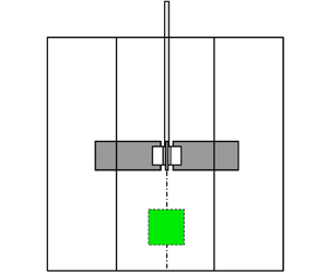
Experiments are carried out with water in the same octagonal acrylic tank originally used by Steiros et al. (Reference Steiros, Bruce, Buxton and Vassilicos2017a,Reference Steiros, Bruce, Buxton and Vassilicosb). The impeller has a radial four-bladed flat-blade turbine, mounted on a stainless steel shaft at the mid-height of the tank; see figure 1(a) where the mixer dimensions are also presented: $D_T$ is the tank diameter (45 cm), $H$ is the tank height ($H = D_T$), $C$ is the rotor height ($H/2$) and $D$ is the rotor diameter (about $D_{T}/2$). Beaumard et al. (Reference Beaumard, Braganća, Cuvier, Steiros and Vassilicos2024) focused on the turbulence in the baffled tank (four vertical bars on the sides of the tank; see figure 1b) because well-designed baffles break the rotation (baffles of width around $0.12D_T$ designed following Nagata (Reference Nagata1975) for close to fully baffled conditions which maximise power consumption and minimise rotation). Here we concentrate on the unbaffled tank (see figure 1a) and use results from the baffled tank only for comparison.

Figure 1. Mixing tank: (a) without baffles; (b) with baffles.

To test the robustness of our results and identify scalings, we run experiments with two different types of blade geometry which stimulate the turbulence differently: rectangular blades of $44\ {\rm mm} \times 99\ {\rm mm}$ size and fractal-like/multiscale blades of the exact same frontal area but much longer perimeter (see more details in Beaumard et al. (Reference Beaumard, Braganća, Cuvier, Steiros and Vassilicos2024)). This change affects significantly the turbulence properties as the turbulence dissipation rate varies by a factor of 2 at iso-rotation speed in the absence of baffles and by nearly a factor of 4 across the four different unbaffled configurations (different blades, different rotation frequencies $F$) considered here (see table 1). We use the two-iteration ‘fractal2’ blade described in Steiros et al. (Reference Steiros, Bruce, Buxton and Vassilicos2017b). Each of the two types of blade is tested with two different rotor speeds (with and without baffles).

Table 1. Main turbulence parameters.

We use two-dimensional two-component (2D2C) PIV in the vertical $(x,z)$ plane ($H$ is along $z$ and $D$ is along $x$ in figure 1a). The field of view is aligned with the vertical plane and the impeller's vertical shaft and has its centre offset by $3 \pm 1\ {\rm mm}$ in the $y$ direction (normal to both $x$ and $z$ directions) from the horizontal position of the shaft at the centre of the tank. Its size is $27\ {\rm mm} \times 28\ {\rm mm}$ and it is placed under the impeller with its centre at a distance of 0.118 m from the bottom of the tank. All details about these experiments are presented in Beaumard et al. (Reference Beaumard, Braganća, Cuvier, Steiros and Vassilicos2024).

The PIV resolution (interrogation window size) is between $3.4\eta$ and $5.1\eta$ depending on the configuration, where the Kolmogorov length $\eta \equiv (\nu ^{3}/\langle \overline {\epsilon ^{\prime }}\rangle )^{1/4}$ is calculated by averaging the turbulence dissipation rate $\epsilon ^{\prime }$ over the PIV field of view (angular brackets) and over time (overbar). To be precise, $\epsilon ^{\prime }$ is the pseudo-dissipation (see Pope Reference Pope2000) estimated from our 2D2C PIV data using its axisymmetric formulation (see Beaumard et al. Reference Beaumard, Braganća, Cuvier, Steiros and Vassilicos2024). Time-resolved measurements were carried out in order to denoise the dissipation from the PIV measurement noise, as explained in the supplementary material of Beaumard et al. (Reference Beaumard, Braganća, Cuvier, Steiros and Vassilicos2024).

For each configuration, 150 000 velocity fields are recorded in time, including 50 000 fully uncorrelated velocity field samples for convergence. This corresponds to a time interval of around 139 min. Averaging over time is not sufficient for convergence and we therefore also apply averaging over space, which greatly improves it. More details about convergence are available in Beaumard et al. (Reference Beaumard, Braganća, Cuvier, Steiros and Vassilicos2024).

The rotation frequency $F$ varies between 1 and 3 Hz (see table 1). The Reynolds number is $Re={2{\rm \pi} F L^2}/{\nu }$, where $L=R=D/2\approx 11.25\ {\rm cm}$ is an estimate of the rotor radius. The value of $Re$ is large, higher than $8 \times 10^4$, and the flow is turbulent. The Rossby number is estimated as $R_O^L={K^{1/2}}/(\varOmega L)$, where $K$ is estimated as $\langle \overline {u_x^{\prime 2}}\rangle + \langle \overline {u_z^{\prime 2}}\rangle$, $R$ is used as an estimate of the integral length scale $L$ of the turbulence and $\varOmega =2{\rm \pi} F$. Our values of $R_O^L$ are around $0.02$ for unbaffled configurations and around $0.06$ for baffled configurations. The smaller Rossby number for the unbaffled cases reflects the fact that the rotation affects the turbulence more for these configurations than for the baffled configurations. However, the rotor angular velocity $\varOmega$ is not representative of the flow rotation in the case of the baffled configurations because the baffles break the flow rotation as explained in Nagata (Reference Nagata1975) (see figure 2). Therefore, the Rossby number is severely underestimated for these configurations and the difference between baffled and unbaffled configurations is much greater than the Rossby number values suggest.

Figure 2. Schematic of mean flow in a mixer with and without baffles (Nagata Reference Nagata1975). The measurement plane is shown as a green square. (a) Flow without baffles. (b) Flow with baffles.

The main turbulent parameters are presented in table 1. They include the turbulence dissipation rate $\langle \overline {\epsilon ^{\prime }}\rangle$ and the Kolmogorov and Taylor length scales $\eta$ and $\lambda$, respectively. Details concerning the calculation of the parameters can be found in Beaumard et al. (Reference Beaumard, Braganća, Cuvier, Steiros and Vassilicos2024).

The Taylor-length-based Reynolds number $Re_{\lambda }$ is larger than 410 in all configurations. Values of $Re_{\lambda }$ are broadly comparable between all configurations, so no significant Reynolds number effect is expected when comparing one with the other.

In figure 3(a), we plot the mean flow velocity for one of our four non-baffled configurations, but the plot is representative of the four configurations. The mean flow velocity is oriented horizontally from right to left and is very small in magnitude. These observations evidence the solid-body rotation identified in Nagata (Reference Nagata1975) and shown schematically in figure 2(a). The solid-body rotation appears in the measurement domain because of the small measurement offset in the $y$ direction. In figure 3(b), we plot the mean flow velocity of one representative baffled configuration. The mean flow velocity is oriented vertically from bottom to top and is significant. This observation is consistent with absence of rotation in the field of view and with the mean flow structure described in Nagata (Reference Nagata1975) and shown in figure 2(b).

Figure 3. Mean flow measurement within the measurement planes shown in figure 2. (a) Rectangular blade without baffles ($F=3\ {\rm Hz}$). (b) Rectangular blade with baffles ($F=1.5\ {\rm Hz}$).

3. Mean flow non-homogeneity and rotation at small scales

The Corrsin length $l_C$ (Corrsin Reference Corrsin1958) was introduced to distinguish between length scales above $l_C$ where mean shear $S$ dominates because its time scale $S^{-1}$ is smaller than the time scale of nonlinear evolution of eddies at such scales and length scales below $l_C$ where the mean flow may be considered locally homogeneous because the nonlinear evolution time scale at such scales is smaller than $S^{-1}$. The Corrsin length aims to assess mean flow non-homogeneity rather than turbulence non-homogeneity, which we evaluate in § 5.

We define an estimate of the Corrsin length as $\widetilde {l_C}=\langle \overline {\epsilon ^{\prime }}\rangle ^{1/2} / \langle S\rangle ^{3/2}$, where

(3.1)\begin{equation} S=\sqrt{ 2\left(\frac{\partial\overline{u_x}}{\partial x}\right)^2 +2\left(\frac{\partial\overline{u_x}}{\partial z}\right)^2 +2\left(\frac{\partial\overline{u_z}}{\partial x}\right)^2 + \left(\frac{\partial\overline{u_z}}{\partial z}\right)^2}, \end{equation}

with $u_x$, $u_y$ and $u_z$ being fluid velocity components in directions $x$, $y$ and $z$, respectively. In practice only the mean flow gradients which we can access either directly or via the assumptions $({\partial \overline { u_x}}/{\partial x})^2 \approx ({\partial \overline { u_y}}/{\partial y})^2$, $({\partial \overline {u_x}}/{\partial z})^2 \approx ({\partial \overline { u_y}}/{\partial z})^2$ and $({\partial \overline { u_z}}/{\partial x})^2 \approx ({\partial \overline { u_z}}/{\partial y})^2$ are taken into account. The terms $({\partial \overline { u_x}}/{\partial y})^2$ and $({\partial \overline {u_y}}/{\partial x})^2$ are not accessible with our PIV and are therefore not taken into account.

The values of $\widetilde {l_C}$ are presented normalised by $\lambda$ in table 2; they are much smaller for the unbaffled than for the baffled configurations, suggesting that mean shear non-homogeneity affects much smaller scales in the absence than in the presence of baffles. The actual values of $\widetilde {l_C}$ are between $3 \lambda$ and $6\lambda$ in the unbaffled configurations, even though § 5 suggests that there can be significant turbulence production at scales smaller than that for these configurations. The exact values of the Corrsin length estimates depend on the choice of formula used to calculate $S$. We should, therefore, be very careful about the interpretation of the actual values of the Corrsin length and focus mainly on its variation between baffled and non-baffled configurations, which should be less dependent on the choice of $S$. The Corrsin length is a very rough and sometimes misleading indicator (see also Chen & Vassilicos Reference Chen and Vassilicos2022) but is nevertheless reliable enough to detect that there is much less mean shear in baffled than in unbaffled flows.

Table 2. Corrsin length estimate $\widetilde {l_C}=\langle \overline {\epsilon ^{\prime }}\rangle ^{1/2} / \langle S\rangle ^{3/2}$ with $S$ defined in (3.1), Zeman scale estimate $\widetilde {l_{\varOmega }}= \langle \overline {\epsilon ^{\prime }}\rangle ^{1/2} / \varOmega ^{3/2}$, $R_O^L={K^{1/2}}/(\varOmega L)$, $L/\widetilde {l_{\varOmega }}$ and $N={K}/(\nu \varOmega)>1$, where $L$ is estimated as $R$ and $K$ is estimated as $\langle \overline {u_x^{\prime 2}}\rangle + \langle \overline {u_z^{\prime 2}}\rangle$.

To identify the length scales affected by rotation, we estimate the Zeman length as $\widetilde {l_{\varOmega }}= \langle \overline {\epsilon ^{\prime }}\rangle ^{1/2} / \varOmega ^{3/2}$. The results normalised by $\lambda$ are presented in table 2. As rotation impacts scales larger than $\widetilde {l_{\varOmega }}$, these results suggest that all scales larger than approximately $0.1 \lambda$ are affected by rotation in the unbaffled cases.

Our values of $\widetilde {l_{\varOmega }}$ in the baffled cases suggest an impact of rotation at scales larger than in the unbaffled cases but still at relatively small scales. However, the actual values of $\widetilde {l_{\varOmega }}$ for the baffled configurations are misleading as the angular velocity $\varOmega$ of the rotor is not representative of the actual rotation in the flow, which is negligible because of the baffles. For the baffled configurations, the rotation is therefore expected to affect only scales much larger than our estimate of $\widetilde {l_{\varOmega }}$ in table 2 and is in fact likely to be negligible at all scales.

Table 2 also shows that the Rossby number $R_O^L$ is smaller than 1 (though underestimated in the baffled cases) and that $L/\widetilde {l_{\varOmega }}$ with the integral scale $L \approx R$ is much larger than 1 (though overestimated in the baffled cases) in all configurations and that $N\equiv {K}/(\nu \varOmega)$ is much larger than 1. We might therefore expect a depletion but not a complete suppression of nonlinearity (see § 5) and a non-Kolmogorov scaling in a range of scales larger than $\widetilde {l_{\varOmega }} \approx \lambda /10$ (see § 4) in the unbaffled configurations which are the main subject of this paper.

4. Second-order structure functions

We now compute and analyse second-order structure functions. For this, we introduce the notation $\delta u_{i}^{\prime }=({u_{i}^{\prime }(\boldsymbol {X}+\boldsymbol {r})-u_{i}^{\prime }(\boldsymbol {X}-\boldsymbol {r})})/{2}$ where $u_{i}^{\prime }$ are the fluctuating velocity components in directions $i=1,2,3$, i.e. directions $x,y,z$, respectively, $\boldsymbol {X}$ is the centroid and $2\boldsymbol {r}$ is the two-point separation vector. We compute the normalised structure functions $\langle \overline {(\delta u_{j}^\prime )^2} / \sqrt {\overline {\epsilon ^{\prime }}F} \rangle$ for $j=1$ (velocity fluctuations along the $x$ axis) and $j=3$ (velocity fluctuations along the $z$ axis) by averaging over time, i.e. over our 150 000 samples (which correspond to 50 000 uncorrelated samples), and also averaging over $\boldsymbol {X}$, i.e. over the planar space of our field of view. The additional averaging over space is necessary for good convergence of our statistics. Note that the structure functions so normalised have dimensions of length.

The normalised structure function $\langle \overline {(\delta u_{x}^\prime )^2} / \sqrt {\overline {\epsilon ^{\prime }}F} \rangle$ is plotted versus $r_x$ and $r_z$ in figure 4(a,b), respectively, for the four unbaffled configurations. We evaluate the spatial average of the ratio $\overline {(\delta u_{x}^\prime )^2} / \sqrt {\overline {\epsilon ^{\prime }}F}$ instead of the ratio of the spatially averaged terms, $\langle \overline {(\delta u_{x}^\prime )^2}\rangle / \sqrt {\langle \overline {\epsilon ^{\prime }} \rangle F}$, in order to take into account the possible non-homogeneous variation of the dissipation over the field of view. This is consistent with the theoretical approach to non-homogeneous turbulence of Chen & Vassilicos (Reference Chen and Vassilicos2022) and Beaumard et al. (Reference Beaumard, Braganća, Cuvier, Steiros and Vassilicos2024) (e.g. see (7.7) in Beaumard et al. (Reference Beaumard, Braganća, Cuvier, Steiros and Vassilicos2024)). A good collapse across configurations and a dimensionally correct linear dependence on both $r_x$ and $r_z$ are observed (hence the normalisation of $r_x$ and $r_z$ with $D$, which is the same in all configurations). The linear interpolation results for $\langle \overline {\delta u_x ^{\prime 2}} \rangle$ in the forms $ar_x +b$ and $ar_z +b$ are presented in tables 3 and 4. These linear interpolations are of very good quality given that the $R^2$ coefficient is larger than $0.9990$ for all configurations. The relative variation of the proportionality coefficient $a$ is relatively small: less than $4\,\%$ in the $r_x$ direction and less than $7\,\%$ in the $r_z$ direction.

Figure 4. Normalised structure function $\langle \overline {(\delta u_{x}^\prime )^2} / \sqrt {\overline {\epsilon ^{\prime }}F}\rangle$ space-averaged over the field of view versus (a) $r_x$ (for $r_z =0$) and (b) $r_z$ (for $r_x =0$). The units on the vertical axes are metres (m). The Taylor length scales of the different configurations are plotted as vertical dashed lines and the Zeman length scales ($\widetilde {l_{\varOmega }}= \langle \overline {\epsilon ^{\prime }}\rangle ^{1/2} / \varOmega ^{3/2}$) as vertical dotted lines.

Table 3. Linear interpolation results of $\langle \overline { \delta u_x ^{\prime 2} } \rangle$ in the $r_x$ direction in the form $a r_x + b$ for the configurations without baffles. The interpolation is done between the Taylor scale $\lambda$ and the largest scale measured. Here $R^2$ is the coefficient of determination.

Table 4. Linear interpolation results of $\langle \overline { \delta u_x ^{\prime 2} } \rangle$ in the $r_z$ direction in the form $a r_z + b$ for the configurations without baffles. The interpolation is done between the Taylor scale $\lambda$ and the largest scale measured. Here $R^2$ is the coefficient of determination.

This differs from the baffled configurations studied in Beaumard et al. (Reference Beaumard, Braganća, Cuvier, Steiros and Vassilicos2024), where power-law behaviours $r_x^{2/3}$ and $r_y^{2/3}$ were found and justified theoretically with a theory initially introduced by Chen & Vassilicos (Reference Chen and Vassilicos2022). However, our finding concerning $\langle \overline {(\delta u_{x}^\prime )^2} / \sqrt {\overline {\epsilon ^{\prime }}F} \rangle$ in rotating non-homogeneous turbulence is very similar to the scaling (1.1) for rotating homogeneous turbulence both because it has the same dependence on $\varOmega$ and the turbulence dissipation rate and because $k^{-2}$ is equivalent to a linear dependence on the two-point separation distance. In agreement with the expectation at the end of the previous section, this is a non-Kolmogorov scaling evidencing a strong and well-defined impact of rotation on the second-order structure function of the horizontal fluctuating velocity component as a function of both $r_x$ and $r_z$. This is also a scaling that is clearly different from helicity cascade scalings such as the one mentioned in the introduction (see Brissaud et al. Reference Brissaud, Frisch, Leorat, Lesieur and Mazure1973; Nazarenko & Laval Reference Nazarenko and Laval2000; Herbert et al. Reference Herbert, Daviaud, Dubrulle, Nazarenko and Naso2012) because it depends on $F$ and the turbulence dissipation rate.

The plots of $\langle \overline {(\delta u_{z}^\prime )^2}/ \overline {\epsilon ^{\prime }}^{1/2} \rangle F^{-1/2}$ in figure 5 do not show good collapse of the fractal and the rectangular blade results. Moreover, the dependencies on $r_x$ and $r_z$ deviate from linear (particularly for the rectangular blades), in agreement with the lack of collapse. Either one or both of $F$ and the turbulence dissipation rate are not involved in the actual scaling of the vertical fluctuating velocity component's second-order structure function or they both are and one additional parameter is needed in the scaling which somehow takes into account differences in the flows generated by fractal and rectangular blade impellers. This is a problem which may require more experiments and which we leave for future research. We did check, however, that the vertical fluctuating velocity component's second-order structure function does not collapse with Kolmogorov scaling and that non-dimensionalisation with $D^2 F^2$ as in Herbert et al. (Reference Herbert, Daviaud, Dubrulle, Nazarenko and Naso2012) rather than with the square roots of the turbulence dissipation and $F$ does not collapse the rectangular and fractal blade results for both $\langle \overline {(\delta u_{x}^\prime )^2} \rangle$ and $\langle \overline {(\delta u_{z}^\prime )^2} \rangle$. This observation suggests that the turbulence dissipation rate depends not only on $F$ and $D$ but also on the geometry of the impeller blades. This is visible in our experiments because of our ability to modify the turbulence dissipation rate by changing the blade geometry without changing the rotation speed and the blade frontal area.

Figure 5. Normalised structure function $\langle \overline {(\delta u_{z}^\prime )^2} / \sqrt {\overline {\epsilon ^{\prime }}F}\rangle$ space-averaged over the field of view versus (a) $r_x$ (for $r_z =0$) and (b) $r_z$ (for $r_x =0$). The units on the vertical axes are metres (m). The Taylor length scales of the different configurations are plotted as vertical dashed lines and the Zeman length scales ($\widetilde {l_{\varOmega }}= \langle \overline {\epsilon ^{\prime }}\rangle ^{1/2} / \varOmega ^{3/2}$) as vertical dotted lines.

Predictions and observations of anisotropic scalings of energy spectra have been made for rapidly rotating homogeneous turbulence (e.g. Galtier Reference Galtier2003; Bellet et al. Reference Bellet, Godeferd, Scott and Cambon2006; Thiele & Müller Reference Thiele and Müller2009). However, even though the scalings of the horizontal fluctuating velocity's structure function are similar in our rotating non-homogeneous turbulence to scalings claimed for rotating homogeneous turbulence (i.e. proportional to $\sqrt {\varOmega }$, the square root of turbulence dissipation and the two-point separation distance), the anisotropy between the scalings of the horizontal and the vertical fluctuating velocity structure functions in our rotating non-homogeneous turbulence bears little resemblance to the spectral anisotropies in rotating homogeneous turbulence. This is an issue which merits future research.

5. Quantification of the different terms of the energy equation

In this section we address the question of the depletion of nonlinearity in rotating non-homogeneous turbulence.

5.1. Kármán–Howarth–Monin–Hill equation

Nonlinearity is responsible for interscale turbulent energy transfers. In the presence of all other coexisting turbulence transfer/transport mechanisms, interscale transfers can be studied in terms of two-point equations derived exactly from the incompressible Navier–Stokes equations (see Hill Reference Hill2001, Reference Hill2002) without any hypotheses or assumptions, in particular no assumptions of homogeneity.

The incompressible Navier–Stokes equation is written at two points $\boldsymbol {\zeta } ^- =\boldsymbol {X}-\boldsymbol {r}$ and $\boldsymbol {\zeta ^+} =\boldsymbol {X}+\boldsymbol {r}$ in physical space, where $\boldsymbol {X}$ is the centroid and $2\boldsymbol {r}$ is the two-point separation vector already introduced in the previous section. One defines the two-point velocity half-difference $\boldsymbol {\delta u}(\boldsymbol {X},\boldsymbol {r},t)\equiv ({\boldsymbol {u}^{+}-\boldsymbol {u}^{-}})/{2}$ and half-sum $\boldsymbol {u_X}(\boldsymbol {X},\boldsymbol {r},t)\equiv ({\boldsymbol {u}^{+}+\boldsymbol {u}^{-}})/{2}$, where $\boldsymbol {u}^{+} \equiv \boldsymbol {u}(\boldsymbol {\zeta ^+})$ and $\boldsymbol {u}^{-} \equiv \boldsymbol {u}(\boldsymbol {\zeta ^-})$ are the fluid velocities at each of the two points, and the two-point pressure half-difference $\delta p (\boldsymbol {X},\boldsymbol {r},t) \equiv ({p^{+}- p^{-}})/{2}$, where $p^{+} \equiv p(\boldsymbol {\zeta ^+})$ and $p^{-} \equiv p (\boldsymbol {\zeta ^-})$ are the pressure-to-density ratios at each of the two points. With a Reynolds decomposition into average plus fluctuating quantities, $\boldsymbol {\delta u} =\bar {\boldsymbol {\delta u}}+\boldsymbol {\delta u}^{\prime }$, $\boldsymbol {u_X} = \overline {\boldsymbol {u_X}} + \boldsymbol {u_X}^{\prime }$ and $\delta p = \delta \bar {p} + \delta p^{\prime }$, where the overline signifies an average over time, the Navier–Stokes equation implies the following KHMH equation (Hill Reference Hill2001, Reference Hill2002; Alves Portela, Papadakis & Vassilicos Reference Alves Portela, Papadakis and Vassilicos2017; Beaumard et al. Reference Beaumard, Braganća, Cuvier, Steiros and Vassilicos2024) under the assumption of statistical stationarity, which applies to our constantly agitated turbulent flow:

(5.1)\begin{align} &\left(\overline{\boldsymbol{u_X}}\boldsymbol{\cdot}\boldsymbol{\nabla_X} +\boldsymbol{\delta\bar{u}}\boldsymbol{\cdot} \boldsymbol{\nabla_r} \right)\frac{1}{2} \overline{|\boldsymbol{\delta u^\prime}|^2} - P_r - P_{Xr}^s + \boldsymbol{\nabla_X}\boldsymbol{\cdot}\left(\overline{\boldsymbol{u_X}^\prime \frac{1}{2}|\boldsymbol{\delta u}^\prime|^2}\right) + \boldsymbol{\nabla_r}\boldsymbol{\cdot}\left(\overline{\boldsymbol{\delta u}^\prime \frac{1}{2}|\boldsymbol{\delta u}^\prime|^2}\right) \nonumber\\ &\quad ={-} \boldsymbol{\nabla_X}\boldsymbol{\cdot}\overline{(\boldsymbol{\delta u ^\prime}\delta p ^\prime)} + \frac{\nu}{2}\boldsymbol{\nabla_X}^2 \frac{1}{2}\overline{|\boldsymbol{\delta u^\prime}|^2} +\frac{\nu}{2}\boldsymbol{\nabla_r}^2 \frac{1}{2}\overline{|\boldsymbol{\delta u^\prime}|^2} -\frac{\nu}{4} \overline{\frac{\partial u_i ^{\prime +}}{\partial \zeta ^+ _k} \frac{\partial u_i ^{\prime +}}{\partial \zeta ^+ _k}}\nonumber\\ &\qquad - \frac{\nu}{4} \overline{\frac{\partial u_i ^{\prime -}}{\partial \zeta ^- _k} \frac{\partial u_i ^{\prime -}}{\partial \zeta ^- _k}}, \end{align}

where $P_r=-\overline {\delta u_j ^\prime \delta u_i ^\prime }({\partial \delta \overline {u_i}}/{\partial r_j})$ and $P_{Xr}^s=-\overline {u_{Xj} ^\prime \delta u_i ^\prime }({\partial \delta \overline {u_i}}/{\partial X_j})$ are small-scale two-point turbulence production rates (see Beaumard et al. Reference Beaumard, Braganća, Cuvier, Steiros and Vassilicos2024).

5.2. Two-point turbulence production rates

We start our data analysis with an assessment of the two-point turbulence production rates. The sums defining $P_r=-\overline {\delta u_j ^\prime \delta u_i ^\prime }({\partial \delta \overline {u_i}}/{\partial r_j})$ and $P_{Xr}^s=-\overline {u_{Xj} ^\prime \delta u_i ^\prime }({\partial \delta \overline {u_i}}/{\partial X_j})$ are sums of nine terms, of which our 2D2C PIV has access to only four. Our data therefore allow only truncations to be calculated directly. The accessible truncation of $P_r$ is

(5.2)\begin{equation} \widetilde{P_r}={-}\overline{\delta u_{x}^{\prime} \delta u_{x}^{\prime}} \frac{\partial \overline{\delta u_{x}}}{\partial r_x} - \overline{\delta u_{x}^{\prime} \delta u_{z}^{\prime}} \frac{\partial \overline{\delta u_{z}}}{\partial r_x} - \overline{\delta u_{z}^{\prime} \delta u_{x}^{\prime}} \frac{\partial \overline{\delta u_{x}}}{\partial r_z} - \overline{\delta u_{z}^{\prime} \delta u_{z}^{\prime}} \frac{\partial \overline{\delta u_{z}}}{\partial r_z}, \end{equation}

with

(5.3)\begin{equation} \overline{\delta u_{y}^{\prime} \delta u_{y}^{\prime}} \frac{\partial \overline{\delta u_{y}}}{\partial r_y} + \overline{\delta u_{x}^{\prime} \delta u_{y}^{\prime}} \frac{\partial \overline{\delta u_{y}}}{\partial r_x} + \overline{\delta u_{x}^{\prime} \delta u_{y}^{\prime}} \frac{\partial \overline{\delta u_{x}}}{\partial r_y} + \overline{\delta u_{z}^{\prime} \delta u_{y}^{\prime}} \frac{\partial \overline{\delta u_{y}}}{\partial r_z} + \overline{\delta u_{z}^{\prime} \delta u_{y}^{\prime}} \frac{\partial \overline{\delta u_{z}}}{\partial r_y} \end{equation}

being the difference between $\widetilde {P_r}$ and $P_r$. Similarly, we have the following truncation estimate of $P_{Xr}^s$:

(5.4)\begin{equation} \widetilde{P_{Xr}^s}={-}\overline{u_{Xx}^{\prime} \delta u_{x}^{\prime}} \frac{\partial \overline{\delta u_{x}}}{\partial X_x} - \overline{u_{Xx}^{\prime} \delta u_{z}^{\prime}} \frac{\partial \overline{\delta u_{z}}}{\partial X_x} - \overline{u_{Xz}^{\prime} \delta u_{x}^{\prime}} \frac{\partial \overline{\delta u_{x}}}{\partial X_z} - \overline{u_{Xz}^{\prime} \delta u_{z}^{\prime}} \frac{\partial \overline{\delta u_{z}}}{\partial X_z}. \end{equation}

Our conclusions for the full two-point turbulence production rates are of course contingent on how closely the truncation estimates capture their behaviour. Even so, our results provide definite insights into the non-homogeneity of the flow and the resulting production physics. We calculate space averages over the field of view of the two truncated two-point production rates ($\langle \widetilde {P_r}\rangle$ and $\langle \widetilde {P_{Xr}^s}\rangle$) and we plot their sum, normalised by $\langle \overline {\epsilon ^{\prime }}\rangle /2$, in figure 6 versus $r_{x}$ and $r_{z}$.

Figure 6. Normalised truncation estimate of the total two-point turbulence production rate $2\langle \widetilde {P_r} + \widetilde {P_{Xr}^s}\rangle /\langle \overline {\epsilon ^{\prime }}\rangle$ versus (a) $r_{x}/\lambda$ (for $r_z =0$) and (b) $r_{z}/\lambda$ (for $r_x =0$).

For all four baffled configurations, the values of $(\langle \widetilde {P_r}\rangle +\langle \widetilde {P_{Xr}^s}\rangle )/\langle \overline {\epsilon ^{\prime }}\rangle$ collapse and are relatively small for most values of $r_x$ and $r_z$ to which our field of view allows access. Whilst $\langle \widetilde {P_r}\rangle +\langle \widetilde {P_{Xr}^s}\rangle$ is negligible at all accessible scales for the unbaffled fractal blade configurations, it is definitely very significant as a fraction of the turbulence dissipation rate for the unbaffled rectangular blade configurations at all scales larger than $\lambda$. This stark non-homogeneity difference between rectangular and fractal blades, perhaps resulting from the fractal blades’ breaking of large-scale coherent structures (Başbuğ, Papadakis & Vassilicos Reference Başbuğ, Papadakis and Vassilicos2018), makes the collapse of the horizontal fluctuating velocity structure functions in figure 4 for all unbaffled configurations all the more remarkable. Even if small-scale turbulence production is negligible in the unbaffled fractal configurations, the turbulence in these configurations is nevertheless non-homogeneous as seen in the remainder of § 5.

5.3. Small-scale linear transport

We now focus on another term of the KHMH equation: the linear spatial transport rate $\overline {\boldsymbol {u_X}}\boldsymbol {{\cdot }}\boldsymbol {\nabla _X} \frac {1}{2} \overline {|\boldsymbol {\delta u^\prime }|^2}$, which is also a term reflecting turbulence non-homogeneity. A non-zero linear spatial transport rate means that two-point turbulent energy ($\frac {1}{2}\overline {|\boldsymbol {\delta u^\prime }|^2}$) enters or leaves the domain with the mean flow. Our 2D2C PIV data allow us to calculate the following truncated estimate of this term: $\langle \widetilde {\overline {\boldsymbol {u_X}}\boldsymbol {{\cdot }}\boldsymbol {\nabla _X}\frac {1}{2} \overline {|\boldsymbol {\delta u^\prime }|^2}}\rangle \equiv \langle ( \overline {u_{Xx}}({\partial }/{\partial X_{x}}) + \overline {u_{Xz}}({\partial }/{\partial X_{z}}))\frac {1}{2} (\overline {\delta u_{x}^{\prime 2} + \delta u_{z}^{\prime 2}})\rangle$. In figure 7, we plot this estimate normalised by $\langle \overline {\epsilon ^{\prime }}\rangle /2$ versus $r_x$ and $r_z$. It appears small compared with $\langle \overline {\epsilon ^{\prime }}\rangle /2$ for all accessible $r_x$ and $r_z$ in all baffled configurations. However, it is not so small compared with $\langle \overline {\epsilon ^{\prime }}\rangle /2$ for most accessible $r_x$ and $r_z$ above $\lambda$ in all unbaffled configurations except the one with rectangular blades and $F=3\ {\rm Hz}$.

Figure 7. Normalised truncation estimate of the linear spatial transport rate $2\langle \widetilde {\overline {\boldsymbol {u_X}}\boldsymbol {{\cdot }}\boldsymbol {\nabla _X}\frac {1}{2} \overline {|\boldsymbol {\delta u^\prime }|^2}}\rangle /\langle \overline {\epsilon ^{\prime }}\rangle$ versus (a) $r_{x}/D$ (for $r_z =0$) and (b) $r_{z}/D$ (for $r_x =0$).

All in all, the non-homogeneity generated by rectangular blades is characterised by a significant two-point turbulence production rate and, depending on $F$, a significant or small two-point linear spatial transport rate. By contrast, the non-homogeneity generated by fractal blades is characterised by a significant two-point linear spatial transport rate but a negligible two-point turbulent production rate. The non-homogeneities generated by these two different types of blade are qualitatively different.

5.4. Energy transfer rate measurements

Given the differences between the structure functions $\langle \overline {\delta u_x ^{\prime 2}} \rangle$ and $\langle \overline {\delta u_z ^{\prime 2}} \rangle$ reported in § 4, we now look at energy transfer rates separately for each of these two structure functions. The KHMH equation (5.1) is the sum over index $i$ of the following three equations (one equation per index $i=1,2,3$):

(5.5)\begin{align} &\left(\overline{\boldsymbol{u_X}}\boldsymbol{\cdot}\boldsymbol{\nabla_X} +\boldsymbol{\delta \bar{u}}\boldsymbol{\cdot}\boldsymbol{\nabla_r} \right)\frac{1}{2} \overline{\delta u_i^{\prime 2}} +\overline{\delta u_j ^\prime \delta u_i ^\prime}\frac{\partial \delta \overline{u_i}}{\partial r_j} +\overline{u_{Xj} ^\prime \delta u_i ^\prime}\frac{\partial \delta \overline{u_i}}{\partial X_j} \nonumber\\ &\qquad + \boldsymbol{\nabla_X}\boldsymbol{\cdot}\left(\overline{\boldsymbol{u_X}^\prime \frac{1}{2}\delta u_i^{\prime 2}}\right) + \boldsymbol{\nabla_r}\boldsymbol{\cdot}\left(\overline{\boldsymbol{\delta u}^\prime \frac{1}{2}\delta u_i^{\prime 2}}\right)\nonumber\\ &\quad ={-} \overline{\delta u_i ^{\prime} \frac{\partial \delta p^{\prime}}{\partial _{Xi}}} + \frac{\nu}{2}\boldsymbol{\nabla_X}^2 \frac{1}{2}\overline{\delta u_i^{\prime 2}} +\frac{\nu}{2}\boldsymbol{\nabla_r}^2 \frac{1}{2}\overline{\delta u_i^{\prime 2}} -\frac{\nu}{4} \overline{\frac{\partial u_i ^{\prime +}}{\partial \zeta ^+ _k} \frac{\partial u_i ^{\prime +}}{\partial \zeta ^+ _k}} - \frac{\nu}{4} \overline{\frac{\partial u_i ^{\prime -}}{\partial \zeta ^- _k} \frac{\partial u_i ^{\prime -}}{\partial \zeta ^- _k}}, \end{align}

with implicit summations over $j$ and over $k$ but not over $i$. These three equations, one per index $i$, hold in them the interscale and interspace transfer rates of two-point turbulent energy in the fluctuating velocity component indexed by $i$. We concentrate on $i=1$ for $\delta u_x ^{\prime 2}$ and $i=3$ for $\delta u_z ^{\prime 2}$.

The limitations of our 2D2C PIV allow us to access truncated estimates of the interscale and interspace transfer rates. In figures 8 and 9, we plot the normalised truncated interscale transfer rates

(5.6)\begin{align} \left.\left\langle \widetilde{\boldsymbol{\nabla_r}\boldsymbol{\cdot} \left(\overline{\boldsymbol{\delta u}^\prime \frac{1}{2} \delta u_x ^{\prime 2} }\right)}\right\rangle\right/\left\langle \frac{1}{2}\overline{\epsilon^{\prime}}\right\rangle \equiv \left.\left\langle\overline{ \delta u_{x} ^{\prime} \frac{\partial}{\partial r_{x}}\frac{1}{2}\delta u_x ^{\prime 2}}\right\rangle\right/\left\langle \frac{1}{2}\overline{\epsilon^{\prime}}\right\rangle + \left.\left\langle \overline{\delta u_{z}^{\prime}\frac{\partial}{\partial r_z}\frac{1}{2}\delta u_x ^{\prime 2}}\right\rangle\right/\left\langle \frac{1}{2}\overline{\epsilon^{\prime}}\right\rangle \end{align}

and

(5.7)\begin{align} \left.\left\langle \widetilde{\boldsymbol{\nabla_r}\boldsymbol{\cdot}\left(\overline{\boldsymbol{\delta u}^\prime \frac{1}{2}\delta u_z ^{\prime 2} }\right)}\right\rangle\right/\left\langle \frac{1}{2}\overline{\epsilon^{\prime}}\right\rangle \equiv \left.\left\langle \overline{ \delta u_{x} ^{\prime} \frac{\partial}{\partial r_{x}}\frac{1}{2}\delta u_z ^{\prime 2}}\right\rangle\right/\left\langle \frac{1}{2}\overline{\epsilon^{\prime}}\right\rangle + \left.\left\langle \overline{\delta u_{z}^{\prime}\frac{\partial}{\partial r_z}\frac{1}{2}\delta u_z ^{\prime 2}}\right\rangle\right/\left\langle\frac{1}{2} \overline{\epsilon^{\prime}}\right\rangle. \end{align}

Figure 8. Space- and time-averaged truncation estimates of the small-scale interscale transfer of the energy contributions $\delta u_x ^{\prime 2}$ and $\delta u_z ^{\prime 2}$ normalised by dissipation and along the $r_x$ direction: (a) $-\langle \widetilde {\boldsymbol {\nabla _r}\boldsymbol {{\cdot }}(\overline {\boldsymbol {\delta u}^\prime \frac {1}{2}\delta u_x ^{\prime 2} })} \rangle / \langle \frac {1}{2}\overline {\epsilon ^{\prime }}\rangle$; (b) $-\langle \widetilde {\boldsymbol {\nabla _r}\boldsymbol {{\cdot }}(\overline {\boldsymbol {\delta u}^\prime \frac {1}{2}\delta u_z ^{\prime 2} })} \rangle / \langle \frac {1}{2}\overline {\epsilon ^{\prime }}\rangle$. Here $r_z =0$.

Figure 9. Space- and time-averaged truncation estimates of the small-scale interscale transfer of the energy contributions $\delta u_x ^{\prime 2}$ and $\delta u_z ^{\prime 2}$ normalised by dissipation and along the $r_z$ direction: (a) $-\langle \widetilde {\boldsymbol {\nabla _r}\boldsymbol {{\cdot }}(\overline {\boldsymbol {\delta u}^\prime \frac {1}{2}\delta u_x ^{\prime 2} })} \rangle / \langle \frac {1}{2}\overline {\epsilon ^{\prime }}\rangle$; (b) $-\langle \widetilde {\boldsymbol {\nabla _r}\boldsymbol {{\cdot }}(\overline {\boldsymbol {\delta u}^\prime \frac {1}{2}\delta u_z ^{\prime 2} })} \rangle / \langle \frac {1}{2}\overline {\epsilon ^{\prime }}\rangle$. Here $r_x =0$.

Similarly, we plot in figures 10 and 11 the normalised truncated interspace transfer rates

(5.8)\begin{align} \left.\left\langle\widetilde{\boldsymbol{\nabla_X}\boldsymbol{\cdot} \left(\overline{\boldsymbol{u_X}^\prime \frac{1}{2}\delta u_x ^{\prime 2}}\right)}\right\rangle\right/\left\langle \frac{1}{2}\overline{\epsilon^{\prime}}\right\rangle \equiv \left.\left\langle \overline{u_{Xx} ^{\prime} \frac{\partial}{\partial X_{x}}\frac{1}{2}\delta u_x ^{\prime 2}}\right\rangle\!\right/\!\left\langle\frac{1}{2}\overline{\epsilon^{\prime}}\right\rangle + \left.\left\langle \overline{u_{Xz}^{\prime} \frac{\partial}{\partial X_z} \frac{1}{2}\delta u_x ^{\prime 2}}\right\rangle\!\right/\!\left\langle \frac{1}{2}\overline{\epsilon^{\prime}}\right\rangle \end{align}

and

(5.9)\begin{align} \left.\left\langle\widetilde{\boldsymbol{\nabla_X}\boldsymbol{\cdot}\left(\overline{\boldsymbol{u_X}^\prime \frac{1}{2} \delta u_z ^{\prime 2}}\right)}\right\rangle\right/\left\langle \frac{1}{2}\overline{\epsilon^{\prime}}\right\rangle \equiv \left.\left\langle \overline{u_{Xx} ^{\prime} \frac{\partial}{\partial X_{x}}\frac{1}{2}\delta u_z ^{\prime 2}}\right\rangle\!\right/\!\left\langle \frac{1}{2}\overline{\epsilon^{\prime}}\right\rangle + \left.\left\langle \overline{u_{Xz}^{\prime} \frac{\partial}{\partial X_z}\frac{1}{2}\delta u_z ^{\prime 2}}\right\rangle\!\right/\!\left\langle \frac{1}{2}\overline{\epsilon^{\prime}}\right\rangle. \end{align}

Figure 10. Space- and time-averaged truncation estimates of the small-scale interspace transfer of the energy contributions $\delta u_x ^{\prime 2}$ and $\delta u_z ^{\prime 2}$ normalised by dissipation and along the $r_x$ direction: (a) $\langle \widetilde {\boldsymbol {\nabla _X}\boldsymbol {{\cdot }}(\overline {\boldsymbol {u_X}^\prime \frac {1}{2}\delta u_x ^{\prime 2} })} \rangle / \langle \frac {1}{2}\overline {\epsilon ^{\prime }}\rangle$; (b) $\langle \widetilde {\boldsymbol {\nabla _X}\boldsymbol {{\cdot }}(\overline {\boldsymbol {u_X}^\prime \frac {1}{2}\delta u_z ^{\prime 2} })} \rangle / \langle \frac {1}{2}\overline {\epsilon ^{\prime }}\rangle$. Here $r_z =0$.

Figure 11. Space- and time-averaged truncation estimates of the small-scale interspace transfer of the energy contributions $\delta u_x ^{\prime 2}$ and $\delta u_z ^{\prime 2}$ normalised by dissipation and along the $r_z$ direction: (a) $\langle \widetilde {\boldsymbol {\nabla _X}\boldsymbol {{\cdot }}(\overline {\boldsymbol {u_X}^\prime \frac {1}{2}\delta u_x ^{\prime 2} })} \rangle / \langle \frac {1}{2}\overline {\epsilon ^{\prime }}\rangle$; (b) $\langle \widetilde {\boldsymbol {\nabla _X}\boldsymbol {{\cdot }}(\overline {\boldsymbol {u_X}^\prime \frac {1}{2} \delta u_z ^{\prime 2} })} \rangle / \langle \frac {1}{2} \overline {\epsilon ^{\prime }}\rangle$. Here $r_x =0$.

We first comment on figures 8 and 9. Our $\delta u_x ^{\prime 2}$ interscale transfer rate estimates (see figures 8a and 9a) suggest that rotation in the unbaffled configurations causes a depletion in the $r_x$ direction and a near-suppression in the $r_z$ direction of interscale transfer nonlinearity (note that depletion of the interscale energy transfer rate does not necessarily indicate depletion of nonlinearity as in the enstrophy transfer range of periodic/homogeneous two-dimensional turbulence, where average interscale energy transfers vanish). With the exception of this near-suppression where $\langle \widetilde {\boldsymbol {\nabla _r}\boldsymbol {{\cdot }}(\overline {\boldsymbol {\delta u}^\prime \frac {1}{2}\delta u_x ^{\prime 2} })}\rangle /\langle \frac {1}{2}\overline {\epsilon ^{\prime }}\rangle$ is close to zero for all accessible values of $r_z$ when $r_x =0$, all our truncation estimates of interscale transfer rates in figures 8 and 9 are negative, suggesting interscale turbulent energy transfers from large to small scales irrespective of configuration. However, whereas the results for the baffled configurations seem to collapse with the normalisation by the turbulence dissipation rate as functions of both $r_{x}/\lambda$ and $r_{z}/\lambda$ and even be approximately constant for $r_x$ and $r_z$ larger than $\lambda$ or a fraction of $\lambda$ (see also Beaumard et al. Reference Beaumard, Braganća, Cuvier, Steiros and Vassilicos2024), for the unbaffled configurations this is only the case for the $\delta u_x ^{\prime 2}$ and not the $\delta u_z ^{\prime 2}$ interscale transfer rates. In fact, the $\delta u_z ^{\prime 2}$ interscale transfer rate (see figures 8b and 9b) not only loses its collapsing scaling with turbulence dissipation rate in the presence of rotation (unbaffled configurations) but also appears intensified by rotation over a range of $r_x$ and $r_z$ scales, particularly around $\lambda$, and decreases with increasing $r_z$ above $\lambda$. In other words, rotation intensifies interscale transfer nonlinearity as far as $\delta u_z ^{\prime 2}$ is concerned and also makes it dependent on $r_x$ and $r_z$. Our results are based on the measured contributions and may not represent the full energy transfers. However, the observed qualitative differences in these contributions between baffled and non-baffled contributions are significant in themselves and demonstrate a clear impact of the flow rotation on interscale turbulent energy transfer rates.

These qualitative differences between $\langle \widetilde {\boldsymbol {\nabla _r}\boldsymbol {{\cdot }}(\overline {\boldsymbol {\delta u}^\prime \frac {1}{2}\delta u_x ^{\prime 2} })}\rangle /\langle \frac {1}{2}\overline {\epsilon ^{\prime }}\rangle$ and $\langle \widetilde {\boldsymbol {\nabla _r}\boldsymbol {{\cdot }}(\overline {\boldsymbol {\delta u}^\prime \frac {1}{2}\delta u_z ^{\prime 2} })}\rangle / \langle \frac {1}{2}\overline {\epsilon ^{\prime }}\rangle$ in the unbaffled configurations echo the fact that there are also differences between the scalings of $\overline {\delta u_x ^{\prime 2}}$ and $\overline {\delta u_z ^{\prime 2}}$ in these configurations as reported in § 4. Interestingly, if the arguments of Kraichnan (Reference Kraichnan1965) and Zhou (Reference Zhou1995) could be translated to low-Rossby-number rotating non-homogeneous turbulence (unbaffled configurations), even though they were developed for low-Rossby-number rotating homogeneous turbulence, it might be possible to claim that $\langle \widetilde {\boldsymbol {\nabla _r}\boldsymbol {{\cdot }}(\overline {\boldsymbol {\delta u}^\prime \frac {1}{2}\delta u_x ^{\prime 2} })}\rangle$ is a function of only the time scale $\varOmega ^{-1}$ and a turbulent energy density $({\rm d}/{\rm d}r_{x})\langle \overline {\delta u_x ^{\prime 2}}\rangle$. Such a claim would act as a bridge between the results in figure 4(a) and the unbaffled results in figure 8(a) because $\langle \overline {\delta u_x ^{\prime 2}}\rangle \sim r_{x} \sqrt {\langle \overline {\epsilon ^{\prime }}\rangle \varOmega }$ (effectively figure 4a) would then imply that $\langle \widetilde {\boldsymbol {\nabla _r}\boldsymbol {{\cdot }}(\overline {\boldsymbol {\delta u}^\prime \frac {1}{2}\delta u_x ^{\prime 2} })}\rangle /\langle \frac {1}{2} \overline {\epsilon ^{\prime }}\rangle$ is a constant independent of $\varOmega$, $r_x$ and impeller blade as figure 8(a) might indeed suggest. It is not clear, though, if and why such an argument might work for the $r_x$ dependence of $\langle \widetilde {\boldsymbol {\nabla _r}\boldsymbol {{\cdot }}(\overline {\boldsymbol {\delta u}^\prime \frac {1}{2} \delta u_x ^{\prime 2} })}\rangle$ and perhaps not for its $r_z$ dependence.

We now comment on figures 10 and 11. Firstly, our truncation estimates of the interspace transport rates of $\delta u_x ^{\prime 2}$ for $r_z =0$ and $r_x \not = 0$ and of $\delta u_z ^{\prime 2}$ for $r_x =0$ and $r_z \not = 0$ appear small for all configurations, both baffled and unbaffled. The comparison of baffled and unbaffled results in figure 11(a) suggests a severe depletion by rotation of the nonlinearity that controls the interspace transport of $\delta u_x ^{\prime 2}$ for $r_x =0$ and any accessible $r_z$. In fact, the rotation seems to lead to near-suppression of the interspace transport of $\delta u_x ^{\prime 2}$ in the fractal blade configurations but may be forcing the interspace transport of $\delta u_x ^{\prime 2}$ to change sign in the rectangular blade configurations at the larger values of $r_z$ (see figure 11a). As already documented earlier in this paper, the non-homogeneity structures of rectangular and fractal blade configurations are different, and this seems to be another difference in their non-homogeneities.

The interspace transport rates in figures 10(b) and 11(a) for the baffled configurations are positive and seem to more or less collapse with turbulence dissipation rate within a range of scales larger than $0.5\lambda$ where the interspace transport rates are about constant. This behaviour has been explained by Beaumard et al. (Reference Beaumard, Braganća, Cuvier, Steiros and Vassilicos2024) on the basis of the theory of Chen & Vassilicos (Reference Chen and Vassilicos2022) and is not the focus of the present work. Here we note that rotation severely modifies this interspace transport behaviour by effectively suppressing the measured contributions to the interspace transport of $\delta u_x ^{\prime 2}$, as already mentioned in the previous paragraph, and by changing the dependence on $r_x$ of the measured contributions to the interspace transport rate of $\delta u_z ^{\prime 2}$ (see figure 10b). The change of behaviour of the measured interspace transport contributions may or may not reflect the behaviour of the full interspace transport rate. However, a clear change compared with the baffled configuration is evidently clear.