2.1. Governing equations

We consider the linear stability of a periodic array of vortices to three-dimensional disturbances in stably stratified and rotating fluids. The effects of density stratification are taken into account by the Boussinesq approximation. Viscosity is taken into account, while diffusion of density is neglected since its effects are negligible (Hattori et al. Reference Hattori, Suzuki, Hirota and Khandelwal2021). The governing equations are

(2.1)$$\begin{gather} \boldsymbol{\nabla}\boldsymbol{\cdot}\boldsymbol{u}=0, \end{gather}$$

(2.2)$$\begin{gather}\frac{\partial{\boldsymbol{u}}}{\partial t}+\boldsymbol{u}\boldsymbol{\cdot}\boldsymbol{\nabla}\boldsymbol{u} + 2\varOmega_0 \boldsymbol{e}_z \times \boldsymbol{u} =-\frac{1}{\rho_0} \boldsymbol{\nabla}{p}-g\frac{\rho}{\rho_0}\boldsymbol{e}_z+\nu \Delta \boldsymbol{u}, \end{gather}$$

(2.3)$$\begin{gather}\frac{\partial{\rho}}{\partial{t}}+\boldsymbol{u}\boldsymbol{\cdot}\boldsymbol{\nabla}{\rho} =0, \end{gather}$$

where $\boldsymbol {u}$, $p$ and $\rho$ are the velocity, pressure and density fields, respectively, $\varOmega _0$ is the angular velocity, $\rho _0$ is a constant reference density, $g$ is the acceleration of gravity and $\nu$ is the kinematic viscosity. We consider high-Reynolds-number flows throughout the paper; in the local stability analysis, we neglect viscous diffusion, while the Reynolds number is set to ${{Re}}=10^5$ in the modal stability analysis.

We consider a 2-D base flow. The vorticity equation for 2-D flows in a rotating frame under the Boussinesq approximation reads

(2.4)\begin{equation} {\dfrac{\partial {\omega_z}}{\partial {t}}} + {\dfrac{\partial {\varPsi}}{\partial {y}}}{\dfrac{\partial {(\omega_z + 2\varOmega_0)}}{\partial {x}}} - {\dfrac{\partial {\varPsi}}{\partial {x}}}{\dfrac{\partial {(\omega_z + 2\varOmega_0)}}{\partial {y}}} = \nu \Delta \omega_z, \end{equation}

where $\varPsi =-\Delta ^{-1}\omega _z$ is the stream function of the base flow. Since $\varOmega _0$ is constant, any 2-D flow that satisfies

(2.5)\begin{equation} {\dfrac{\partial {\varPsi}}{\partial {y}}}{\dfrac{\partial {\omega_z}}{\partial {x}}} - {\dfrac{\partial {\varPsi}}{\partial {x}}}{\dfrac{\partial {\omega_z}}{\partial {y}}} = 0 \end{equation}

is steady in the absence of viscous diffusion. Equation (2.5) is the well-known condition for 2-D steady inviscid flows without rotation and stratification. In other words, rotation and stratification do not affect the condition for steadiness under the Boussinesq approximation and uniform rotation.

The base flow is assumed steady not only in local stability analysis but also in modal stability analysis because the growth of instabilities is much faster than the time evolution of the base flow due to viscous diffusion at ${{Re}}=10^5$. The velocity, pressure and density fields are decomposed as

(2.6)$$\begin{gather} \boldsymbol{u}=\boldsymbol{u}_b+\boldsymbol{u}', \end{gather}$$

(2.7)$$\begin{gather}p=p_b+p', \end{gather}$$

(2.8)$$\begin{gather}\rho=\rho_{0}+{\alpha}z+\rho', \end{gather}$$

where $(\boldsymbol {u}_b, p_b, \rho _b)$ and $(\boldsymbol {u}', p', \rho ')=(u'_x, u'_y, u'_z, p', \rho ')$ are the base flow and the disturbance, the direction of the gravity force is taken as $-\boldsymbol {e}_z$ and the base density is assumed to be $\rho _b=\rho _0+\alpha z$ with $\alpha ={\partial \rho _b}/{\partial z}<0$ being a constant. The magnitude of the disturbance is infinitesimally small. Then the governing equations of the disturbance in non-dimensionalized form are

(2.9)$$\begin{gather} \boldsymbol{\nabla}\boldsymbol{\cdot}\boldsymbol{u}'=0, \end{gather}$$

(2.10)$$\begin{gather}\frac{\partial{\boldsymbol{u}'}}{\partial t}+(\boldsymbol{u}'\boldsymbol{\cdot}\boldsymbol{\nabla})\boldsymbol{u}_b+(\boldsymbol{u}_b\boldsymbol{\cdot}\boldsymbol{\nabla})\boldsymbol{u}' + \frac{1}{Ro} \boldsymbol{e}_z \times \boldsymbol{u}' =-\boldsymbol{\nabla}{p'}-\rho'\boldsymbol{e}_z+\frac{1}{{{Re}}}\nabla^2 \boldsymbol{u}', \end{gather}$$

(2.11)$$\begin{gather}\frac{\partial{\rho'}}{\partial{t}}+(\boldsymbol{u}_b\boldsymbol{\cdot}\boldsymbol{\nabla}){\rho'}-\frac{1}{F_h^2}u'_z =0, \end{gather}$$

where $Ro =U_0/(2 \varOmega _0 L_0)$ is the Rossby number, ${{Re}} =U_0L_0/\nu$ is the Reynolds number, $F_h=U_0/(L_0N)$ is the Froude number based on the horizontal scale, $N=\sqrt {-{\alpha }g/{\rho }_0}$ is the Brunt–Väisälä frequency, and $U_0$ and $L_0$ are a characteristic velocity and a length scale, respectively; see § 4 for the actual choice of $U_0$ and $L_0$. In the following, the values are scaled by $U_0$ and $L_0$ unless stated explicitly.

In the local stability analysis, the disturbance is assumed to be in the form of a wave packet with short wavelength:

(2.12)$$\begin{gather} \boldsymbol{u}'=\left(\boldsymbol{\hat{u}}_0+\delta\boldsymbol{\hat{u}}_1+\cdots \right)\exp\left(\frac{{\rm i}}{\delta}\varPhi\right), \end{gather}$$

(2.13)$$\begin{gather}p'=\left(\hat{p}_0+\delta\hat{p}_1+\cdots \right)\exp\left(\frac{{\rm i}}{\delta}\varPhi\right), \end{gather}$$

(2.14)$$\begin{gather}\rho'=\left(\hat{\rho}_0+\delta\hat{\rho}_1+\cdots \right)\exp\left(\frac{{\rm i}}{\delta}\varPhi\right), \end{gather}$$

where $\delta$ is a small parameter proportional to the wavelength and $\varPhi$ is eikonal which is assumed to satisfy $D\varPhi /Dt=0$ ($D/Dt=\partial /\partial t+ \boldsymbol {u}_b \boldsymbol {\cdot } \boldsymbol {\nabla }$). Viscosity is neglected in the local stability analysis. Substituting the above expressions into (2.9)–(2.11) yields a set of ordinary differential equations at the leading order:

(2.15)$$\begin{gather} {\dfrac{{\rm{d}} {{\boldsymbol{X}}}}{{\rm{d}} {t}}} = {\boldsymbol{U}}({\boldsymbol{X}}), \end{gather}$$

(2.16)$$\begin{gather}{\dfrac{{\rm{d}} {{\boldsymbol{k}}}}{{\rm{d}} {t}}} =-{\boldsymbol{\mathsf{L}}}^{\rm T} {\boldsymbol{k}}, \end{gather}$$

(2.17)$$\begin{gather}{\dfrac{{\rm{d}} {{\boldsymbol{a}}}}{{\rm{d}} {t}}} = ( 2{\hat{\boldsymbol{k}}}{\hat{\boldsymbol{k}}}^{\rm T} - {\boldsymbol{\mathsf{I}}} ) {\boldsymbol{\mathsf{L}}}{\boldsymbol{a}} +({\hat{\boldsymbol{k}}}{\hat{\boldsymbol{k}}}^{\rm T}-{\boldsymbol{\mathsf{I}}})r\boldsymbol{e}_z + \frac{1}{Ro} ( {\hat{\boldsymbol{k}}}{\hat{\boldsymbol{k}}}^{\rm T} - {\boldsymbol{\mathsf{I}}} ) {\boldsymbol{e}_z} \times {\boldsymbol{a}}, \end{gather}$$

(2.18)$$\begin{gather}\frac{{\rm d}r}{{\rm d}t}= \frac{1}{F_h^2}a_z, \end{gather}$$

where $\boldsymbol{\mathsf{L}}_{ij} = {\partial U_i}/{\partial x_j}$ and $\hat {\boldsymbol {k}}=\boldsymbol {k}/|{\boldsymbol {k}}|$ (Friedlander & Vishik Reference Friedlander and Vishik1991; Lifschitz & Hameiri Reference Lifschitz and Hameiri1991; Leblanc Reference Leblanc1997). Here, ${\boldsymbol {X}}$ is the position of the fluid particle and $\boldsymbol {k}=\boldsymbol {\nabla }\varPhi$ is the local wavevector, while ${\boldsymbol {a}}=\boldsymbol {\hat {u}}_0$ and $r=\hat {\rho }_0$ are the amplitudes of the disturbance corresponding to velocity and density, respectively. The incompressibility condition in (2.9) leads to ${\boldsymbol {a}} \boldsymbol {\cdot } {\boldsymbol {k}} = 0$, which is satisfied for $t>0$ if it holds at $t=0$. The base flow is unstable if the amplitude $\{{\boldsymbol {a}}, r\}$ grows without bound.

2.2. Useful equations and approximations

Before showing the condition for each instability and the estimate of the growth rate, useful equations and approximations are presented. We are left with four (2.17) and (2.18) after solving (2.15) and (2.16). The incompressibility condition ${\boldsymbol {a}} \boldsymbol {\cdot } {\boldsymbol {k}} = 0$ implies that the actual degree of freedom is three; it is further reduced to two using conservation of potential vorticity (Aspden & Vanneste Reference Aspden and Vanneste2009; Suzuki et al. Reference Suzuki, Hirota and Hattori2018).

First, we introduce

(2.19a–c)\begin{equation} p = \frac{k}{|\boldsymbol{k}_\perp|} {\boldsymbol{k}}_\perp \boldsymbol{\cdot} {\boldsymbol{a}}_\perp = -\frac{kk_z}{|\boldsymbol{k}_\perp|}a_z, \quad q = \left(\frac{k}{|\boldsymbol{k}_\perp|} {\boldsymbol{k}}_\perp{\times} {\boldsymbol{a}}_\perp\right)\boldsymbol{\cdot}{\boldsymbol{e}}_z, \quad s = \frac{k}{|\boldsymbol{k}_\perp|}r \end{equation}

as done by Bayly, Holm & Lifschitz (Reference Bayly, Holm and Lifschitz1996), where $\boldsymbol {k}_\perp =(k_x, k_y)^{\rm T}$ and $\boldsymbol {a}_\perp =(a_x, a_y)^{\rm T}$ are the horizontal projections of $\boldsymbol {k}$ and $\boldsymbol {a}$, respectively. Then, (2.17) and (2.18) reduce to

(2.20) \begin{equation} \frac{{\rm d}}{{\rm d}t}\left( \begin{array}{@{}c@{}}p\\q\\s\end{array}\right) = \left( \begin{array}{@{}ccc@{}} \dfrac{{\rm d}}{{\rm d}t}\log{\dfrac{|\boldsymbol{k}_\perp|}{|\boldsymbol{k}|}} & \dfrac{2k^2_z\boldsymbol{\mathsf{H}}\boldsymbol{k}_\perp\boldsymbol{\cdot}\boldsymbol{k}_\perp}{|\boldsymbol{k}|^2|\boldsymbol{k}_\perp|^2} +\dfrac{k_z^2}{Ro k^2} & \dfrac{|\boldsymbol{k}_\perp|^2}{|\boldsymbol{k}|^2}k_z\\ -\omega_z-{{{Ro}}^{-1}} & -\dfrac{{\rm d}}{{\rm d}t}\log{\dfrac{|\boldsymbol{k}_\perp|}{|\boldsymbol{k}|}} & 0\\ -\dfrac{1}{F_h^2 k_z} & 0 & -\dfrac{{\rm d}}{{\rm d}t}\log{\dfrac{|\boldsymbol{k}_\perp|}{|\boldsymbol{k}|}}\\ \end{array}\right) \left( \begin{array}{@{}c@{}} p\\q\\s\end{array}\right), \end{equation}

where

(2.21a,b)\begin{equation} {\boldsymbol{\mathsf{L}}} = \left( \begin{array}{@{}cc@{}} {\boldsymbol{\mathsf{L}}}_\perp & 0 \\ 0 & 0 \end{array} \right), \quad \boldsymbol{\mathsf{H}} = \boldsymbol{\mathsf{L}}_\perp \left( \begin{array}{@{}cc@{}} 0 & 1 \\ -1 & 0 \end{array} \right). \end{equation}

By eliminating $p$ from the equations for $p$ and $q$, we have

(2.22)\begin{equation} {\dfrac{{\rm{d}}^2 {q}}{{\rm{d}} {t}^2}} = U_q q + D_s s, \end{equation}

where

(2.23)$$\begin{gather} U_q = \left(\frac{{\rm d}}{{\rm d}t}\log{\frac{|\boldsymbol{k}_\perp|}{|\boldsymbol{k}|}}\right)^2 - \frac{{\rm d}^2}{{\rm d}t^2}\log{\frac{|\boldsymbol{k}_\perp|}{|\boldsymbol{k}|}} - \left(\frac{2k^2_z\boldsymbol{\mathsf{H}}\boldsymbol{k}_\perp\boldsymbol{\cdot}\boldsymbol{k}_\perp}{|\boldsymbol{k}|^2|\boldsymbol{k}_\perp|^2} +\frac{k_z^2}{Ro k^2}\right)(\omega_z+{{{Ro}}^{-1}} ), \end{gather}$$

(2.24)$$\begin{gather}D_s=-\frac{|\boldsymbol{k}_\perp|^2}{|\boldsymbol{k}|^2}k_z (\omega_z+{{{Ro}}^{-1}} ). \end{gather}$$

We can also eliminate $p$ from the equations for $q$ and $s$, which leads to

(2.25)\begin{equation} {\dfrac{{\rm{d}} {q}}{{\rm{d}} {t}}} -F_h^2(\omega_z+{{{Ro}}^{-1}})k_z {\dfrac{{\rm{d}} {s}}{{\rm{d}} {t}}} =-\left(\frac{{\rm d}}{{\rm d}t}\log{\frac{|\boldsymbol{k}_\perp|}{|\boldsymbol{k}|}}\right) (q - F_h^2(\omega_z+{{{Ro}}^{-1}})k_z s). \end{equation}

Since $\omega _z$ and $k_z$ are constant along a streamline, we have

(2.26)\begin{equation} {\dfrac{{\rm{d}} {}}{{\rm{d}} {t}}} \left[\left(\frac{|\boldsymbol{k}_\perp|}{|\boldsymbol{k}|}\right) (q - F_h^2(\omega_z+{{{Ro}}^{-1}})k_z s)\right] = 0 \end{equation}

or

(2.27)\begin{equation} q - F_h^2(\omega_z+{{{Ro}}^{-1}})k_z s = C_{pv}\frac{|\boldsymbol{k}|}{|\boldsymbol{k}_\perp|}, \end{equation}

where $C_{pv}$ is a constant. For an unstable solution which grows exponentially, the right-hand side of (2.27) can be neglected so that we have

(2.28)\begin{equation} q = F_h^2(\omega_z+{{{Ro}}^{-1}})k_z s. \end{equation}

Then the equation for $q$ becomes a closed equation

(2.29)\begin{equation} {\dfrac{{\rm{d}}^2 {q}}{{\rm{d}} {t}^2}} = V_q q, \end{equation}

where

(2.30)\begin{align} V_q &= \left(\frac{{\rm d}}{{\rm d}t}\log \sin \theta \right)^2 - \frac{{\rm d}^2}{{\rm d}t^2}\log \sin \theta \nonumber\\ &\quad - (2\boldsymbol{\mathsf{H}}\hat{\boldsymbol{k}}_\perp\boldsymbol{\cdot}\hat{\boldsymbol{k}}_\perp \cos^2\theta +Ro^{-1}\cos^2\theta )(\omega_z+{{{Ro}}^{-1}})-F_h^{-2}\sin^2\theta, \end{align}

and $\theta =\cos ^{-1} k_z/|\boldsymbol {k}|$ is the angle of wavevector and $\hat {\boldsymbol {k}}_\perp =\boldsymbol {k}_\perp /|\boldsymbol {k}_\perp |$. We use (2.29) in some of the following subsections.

3.1. Pure hyperbolic instability

The pure hyperbolic (PH) instability is due to stretching near the hyperbolic stagnation points (Friedlander & Vishik Reference Friedlander and Vishik1991; Lifschitz & Hameiri Reference Lifschitz and Hameiri1991; Leblanc Reference Leblanc1997). The mechanism and the growth rate can be estimated analytically by investigating the solution to (2.17) at the hyperbolic stagnation points. We set $\theta =0^\circ$ or ${\boldsymbol {k}}_\perp =0$ for which the growth rate is maximum and stratification has no effect as will be confirmed in § 5. Then the equation for ${\boldsymbol {a}}_\perp$ reads

(3.1)\begin{equation} {\dfrac{{\rm{d}} {{\boldsymbol{a}}_\perp}}{{\rm{d}} {t}}} = \left( \begin{array}{@{}cc@{}} -{\dfrac{\partial {u_b}}{\partial {x}}} & -{\dfrac{\partial {u_b}}{\partial {y}}} + {{{Ro}}^{-1}} \\ -{\dfrac{\partial {v_b}}{\partial {x}}}- {{{Ro}}^{-1}} & -{\dfrac{\partial {v_b}}{\partial {y}}} \end{array} \right) \left( \begin{array}{@{}c@{}} a_x \\ a_y \end{array} \right). \end{equation}

Let us consider a hyperbolic stagnation point where the flow is expanded as $(u_b, v_b) = \varepsilon _h (x, -y) + O(x^2+y^2)$. Then the above equation becomes

(3.2) \begin{equation} {\dfrac{{\rm{d}} {{\boldsymbol{a}}_\perp}}{{\rm{d}} {t}}} = \left( \begin{array}{@{}cc@{}} -\varepsilon_h & {{{Ro}}^{-1}} \\ -{{{Ro}}^{-1}} & \varepsilon_h \end{array} \right) \left( \begin{array}{@{}c@{}} a_x \\ a_y \end{array} \right), \end{equation}

where $\varepsilon _h={\partial u_b}/{\partial x}=-({\partial v_b}/{\partial y})$ is the strain rate. The eigenvalues of the matrix in (3.2) are given by

(3.3)\begin{equation} \lambda^2 = \varepsilon_h^2-{Ro}^{-2}. \end{equation}

Thus, the pure hyperbolic instability occurs when $|{{{Ro}}^{-1}}| < \varepsilon _h$. The above (3.2) has a simple solution:

(3.4a,b)\begin{equation} a_x = a_x(0) {\rm e}^{-\varepsilon_h t}, \quad a_y = a_y(0) {\rm e}^{\varepsilon_h t}, \end{equation}

when ${{{Ro}}^{-1}}=0$ (Friedlander & Vishik Reference Friedlander and Vishik1991; Lifschitz & Hameiri Reference Lifschitz and Hameiri1991). In this regard, $a_y$ is in the stretching phase, while $a_x$ is in the compression phase. However, when the fluid particle is away from the hyperbolic stagnation points so that the strain rate is small, the phase of $\boldsymbol {a}$ changes approximately as $\boldsymbol {a} \propto {\rm e}^{\pm {\rm {i}} {{{Ro}}^{-1}} t}$, which we call the oscillation phase below.

In general, an estimate for the growth rate on a closed streamline is required. In this case, we should take into account that the wave packet does not always grow with the eigenvalue $\lambda$; it is either stretched or compressed near the hyperbolic stagnation points depending on the direction of $\boldsymbol {a}$; when it is away from the hyperbolic stagnation points, the direction of $\boldsymbol {a}$ rotates in the oscillation phase. Therefore, the growth rate is estimated as $\sigma = C_{PH}(\varepsilon _h^2-{Ro}^{-2})^{1/2}$, where $C_{PH} \lesssim 1$ is a coefficient determined by the ratio of time of the stretching phase, in which the fluid particle stays near the stagnation points, and the oscillation phase, in which the fluid particle travels between the stagnation points. In the short-wave limit, the instability condition and the growth rate are unaffected by stratification because it occurs for $\theta =0^\circ$ where the stratification effects vanish.

3.2. Strato-hyperbolic instability

The strato-hyperbolic (SH) instability is a variant of the pure hyperbolic instability under stratification effects; it occurs when the exponential growth near the hyperbolic stagnation points is connected with phase shift due to the gravity waves in favour of exponential growth. Although the waves become inertia-gravity waves under rotation effects, the condition and the growth rate are estimated similarly as for the pure hyperbolic instability; the growth rate is estimated as $\sigma = C_{SH}(\varepsilon _h^2-{Ro}^{-2})^{1/2}$; it is stabilized when $|{{{Ro}}^{-1}}| > \varepsilon _h$. The coefficient $C_{SH}$ is smaller than $C_{PH}$ in general because the ratio of the stretching phase to the oscillation phase decreases for larger $\theta$, where the strato-hyperbolic instability occurs. One important difference, however, is that the frequency of the gravity wave should be large enough to generate the phase shift during the fluid particle motion where the frequency is approximated as $\omega _{max}/2$; this leads to ${F_h^{-1}} \gtrsim \omega _{max}/2$ as an instability condition (Suzuki et al. Reference Suzuki, Hirota and Hattori2018). The resonance condition for the instability derived by Suzuki et al. (Reference Suzuki, Hirota and Hattori2018) can be generalized as

(3.5)\begin{equation} \int_{0}^{T/2} \sqrt{Ro^{-2}\cos^2 \theta + F_h^{-2} \sin^2 \theta} \,{\rm d}t = m {\rm \pi}, \end{equation}

where $T$ is the period of fluid particle motion and $m$ is a positive integer. When ${F_h^{-1}}$ is large, the left-hand side of the above equation increases monotonically with $\theta _0$, so that the resonance condition is satisfied for $|{{{Ro}}^{-1}}| \lesssim 2m{\rm \pi} /T \lesssim {F_h^{-1}}$; thus, the strato-hyperbolic instability exists in the limit of strong stratification.

3.3. Rotational-hyperbolic instability

Although the pure hyperbolic instability is stabilized for $|{{{Ro}}^{-1}}| > \varepsilon _h$, the potential $V_q$ in (2.29) oscillates periodically along streamlines near the cell boundaries. In fact, $V_q$ is approximated as

(3.6)\begin{equation} V_q \approx-{\dfrac{{\rm{d}}^2 {}}{{\rm{d}} {t}^2}} \log \sin \theta - {Ro}^{-2} \cos^2\theta - F_h^{-2} \sin^2\theta \end{equation}

near the cell boundaries; the first term is the main source of oscillation, while the other terms are responsible for the inertia-gravity waves. This oscillation can resonate with the inertia-gravity waves to give rise to another instability; we call it rotational-hyperbolic (RH) instability because it is the motion near the hyperbolic points which is responsible for the oscillation of $V_q$. This instability has been shown by Sipp et al. (Reference Sipp, Lauga and Jacquin1999) without much attention and found by Godeferd et al. (Reference Godeferd, Cambon and Leblanc2001) both by local stability analysis, while its nature should be further explored because the corresponding unstable mode has not been found in modal stability analysis. Since the time period of the fluid particle motion is large on streamlines near the cell boundaries, the resonance occurs for small frequency of the inertia-gravity waves: $\theta \approx {\rm \pi}/2$ and small ${F_h^{-1}}$. The growth rate is estimated as $\sigma = C_{RH} \varepsilon _h$, where $C_{RH}$ is in general smaller than $C_{PH}$ since the wavevector angle $\theta$ is larger than the pure hyperbolic instability. The resonance condition for the rotational-hyperbolic instability is the same as (3.5) for the strato-hyperbolic instability; since it is satisfied for $\min (|{{{Ro}}^{-1}}|,{F_h^{-1}}) \lesssim 2m{\rm \pi} /T \lesssim \max (|{{{Ro}}^{-1}}|,{F_h^{-1}})$, the rotational-hyperbolic instability exists in the limit of strong stratification or rotation, although the growth rate becomes small for higher resonance (large $m$).

3.4. Centrifugal instability

The centrifugal (C) instability has been studied extensively since the discovery of the Rayleigh criterion (Rayleigh Reference Rayleigh1917); a criterion for rotating fluids was derived by Kloosterziel & van Heijst (Reference Kloosterziel and van Heijst1991). We set $\theta =0^\circ$ or ${\boldsymbol {k}}_\perp =0$ where the growth rate is maximum and stratification has no effect. In addition, we approximate the base flow by an axisymmetric flow

(3.7)\begin{equation} \boldsymbol{U}=U_\varTheta^{(0)}(R) {\boldsymbol{e}}_{\varTheta} \end{equation}

in the polar coordinates $(R, \varTheta )$ centred at an elliptic stagnation point to obtain concise expressions for the instability condition and growth rate. Then the equation for ${\boldsymbol {a}}_\perp =a_R{\boldsymbol {e}}_{R}+a_\varTheta {\boldsymbol {e}}_{\varTheta }$ reads

(3.8) \begin{equation} {\dfrac{{\rm{d}} {}}{{\rm{d}} {t}}} \left( \begin{array}{@{}c@{}} a_R \\ a_\varTheta \end{array} \right) + \varOmega_p \left( \begin{array}{@{}c@{}} -a_\varTheta \\ a_R \end{array} \right) = \left( \begin{array}{@{}cc@{}} 0 & \varOmega_p + {{{Ro}}^{-1}} \\ -{\dfrac{{\rm{d}} {U_\varTheta^{(0)}}}{{\rm{d}} {R}}}- {{{Ro}}^{-1}} & 0 \end{array} \right) \left( \begin{array}{@{}c@{}} a_R \\ a_\varTheta \end{array} \right), \end{equation}

where $\varOmega _p={U_\varTheta ^{(0)}}/{R}$ is the rotation rate of a fluid particle. The above equation is reduced to

(3.9)\begin{equation} {\dfrac{{\rm{d}}^2 {a_R}}{{\rm{d}} {t}^2}} =-2\left(\varOmega_p + \frac{{{{Ro}}^{-1}}}{2} \right) (\omega_z+{{{Ro}}^{-1}}) a_R, \end{equation}

where $\omega _z={{\rm {d}}U_\varTheta ^{(0)}}/{{\rm {d}}R}+{U_\varTheta ^{(0)}}/{R}$ is the vorticity. Thus, the Rayleigh criterion in rotating fluids is recovered as the condition for the centrifugal instability:

(3.10)\begin{equation} \left(\varOmega_p + \frac{{{{Ro}}^{-1}}}{2} \right) (\omega_z+{{{Ro}}^{-1}}) < 0 \end{equation}

or

(3.11)\begin{equation} -2\varOmega_p < {{{Ro}}^{-1}} <- \omega_z \end{equation}

on each streamline. We assume that $\omega _z$ decreases monotonically with $R$ and $\omega _z\ge 0$. Then, $\varOmega _p$ is maximum at $R=0$ where $2\varOmega _p=\omega _z(0)=\omega _{max}$, by which the instability condition becomes

(3.12)\begin{equation} -\omega_{max} < {{{Ro}}^{-1}} < 0. \end{equation}

The maximum growth rate depends on the vorticity distribution. The growth rate at a given streamline takes the maximum value when $-{{{Ro}}^{-1}}=\varOmega _p(R)+\omega _z(R)/2$:

(3.13)\begin{equation} \sigma = \varOmega_p-\frac{\omega_z}{2} = C_C \omega_{max}, \end{equation}

where $C_C$ is an $O(1)$ coefficient.

3.5. Elliptic instability

The elliptic (E) instability in rotating stratified fluids was studied by Kerswell (Reference Kerswell2002) and Leblanc (Reference Leblanc2003) for the unbounded case, and by Guimbard et al. (Reference Guimbard, Le Dizès, Le Bars, Le Gal and Leblanc2010) for the flow inside a rotating cylinder; see also Godeferd et al. (Reference Godeferd, Cambon and Leblanc2001) for the rotating non-stratified case and Miyazaki & Fukumoto (Reference Miyazaki and Fukumoto1992) for the non-rotating stratified case. Here we derive a new result required for interpretation of the results in § 5 after recovering the results obtained by Kerswell (Reference Kerswell2002) and Leblanc (Reference Leblanc2003).

We assume that the base flow is a sum of an axisymmetric flow and a weak straining flow:

(3.14)\begin{equation} \boldsymbol{U}=U_\varTheta^{(0)}(R) {\boldsymbol{e}}_{\varTheta} + \varepsilon_e \left[U_R^{(1)}(R) \sin 2\varTheta {\boldsymbol{e}}_{r} +U_\varTheta^{(1)}(R) \cos 2\varTheta {\boldsymbol{e}}_{\varTheta}\right]. \end{equation}

The potential in (2.29) turns out to be

(3.15)\begin{align} V_q &=V_q^{(0)} + \varepsilon_e V_{q}^{(1)} \cos 2\varOmega_p t + O(\varepsilon_e^2), \end{align}

(3.16)\begin{align} V_q^{(0)} &=-(2\varOmega_p+{{{Ro}}^{-1}})(\omega_z+{{{Ro}}^{-1}}) \cos^2\theta -F_h^{-2}\sin^2\theta, \end{align}

(3.17)\begin{align} V_{q}^{(1)} &= 2 \varOmega_p \cos^2\theta \left( \frac{U_R^{(1)}}{R_0} +{\dfrac{{\rm{d}} {U_R^{(1)}}}{{\rm{d}} {R}}} -\frac{U_R^{(1)}}{R_0\varOmega_p} {\dfrac{{\rm{d}} {U_\varTheta^{(0)}}}{{\rm{d}} {R}}}\right) -2 \cos^2\theta (\omega_z+{{{Ro}}^{-1}}) \nonumber\\ & \quad + \left[ -\gamma \sin^2\theta {\dfrac{{\rm{d}} {U_R^{(1)}}}{{\rm{d}} {R}}} -\left(\frac{3}{2}+\gamma\sin^2\theta\right) \frac{U_R^{(1)}}{R_0}\right. \notag\\ &\quad + \left. \frac{U_\varTheta^{(1)}}{R_0} +\left(-\frac{1}{2}+\gamma\sin^2\theta\right) \frac{U_R^{(1)}}{R_0\varOmega_p}{\dfrac{{\rm{d}} {U_\varTheta^{(0)}}}{{\rm{d}} {R}}}\right] \nonumber\\ & \quad -\frac{\sin^2\theta \cos^2\theta}{F_h^2\varOmega_p}\left( \frac{U_R^{(1)}}{R_0} +{\dfrac{{\rm{d}} {U_R^{(1)}}}{{\rm{d}} {R}}} -\frac{U_R^{(1)}}{R_0\varOmega_p} {\dfrac{{\rm{d}} {U_\varTheta^{(0)}}}{{\rm{d}} {R}}}\right), \end{align}

where $\gamma = 1 + 1/(2Ro \varOmega _p)$. The leading-order term determines the oscillation frequency $\omega$ by $\omega ^2=-V_q^{(0)}$, while the first-order term can induce resonance so that an instability occurs.

First, we focus on the stability near the elliptic stagnation points. At $R \approx 0$, $\omega _z \approx 2\varOmega _p \approx \omega _{max}$, which gives

(3.18)\begin{equation} \omega^2 =-V_q^{(0)} \approx (\omega_{max}+{{{Ro}}^{-1}})^2 \cos^2\theta +F_h^{-2}\sin^2\theta. \end{equation}

The resonance condition is

(3.19)\begin{equation} \omega = \frac{n}{2} \omega_{max}, \end{equation}

which gives, for $n=1$,

(3.20)\begin{equation} \cos^2\theta = \frac{1}{4} \frac{\omega_{max}^2-4F_h^{-2}}{(\omega_{max}+{{{Ro}}^{-1}})^2-F_h^{-2}}. \end{equation}

When (3.20) has a solution, the growth rate is obtained as

(3.21)\begin{equation} \sigma = \frac{\varepsilon_e}{64} \left|\frac{(\omega_{max}^2-4F_h^{-2})\left(3\omega_{max}+2{{{Ro}}^{-1}}\right)^2}{\left[(\omega_{max}+{{{Ro}}^{-1}})^2-F_h^{-2}\right] \omega_{max}^2} \right|, \end{equation}

which recovers the result by Leblanc (Reference Leblanc2003) with $\omega _{max}=2, {{{Ro}}^{-1}}=2f, F_h^{-1}=2n$ and $\varepsilon =\delta /2$. The instability condition is obtained by considering $0 \le \cos ^2\theta \le 1$ in (3.20): when ${F_h^{-1}}<\omega _{max}/2$,

(3.22)\begin{equation} {{{Ro}}^{-1}} <-\tfrac{3}{2} \omega_{max} \quad \text{or} \quad {{{Ro}}^{-1}} >-\tfrac{1}{2} \omega_{max}, \end{equation}

and when ${F_h^{-1}}>\omega _{max}/2$,

(3.23)\begin{equation} -\tfrac{3}{2} \omega_{max} < {{{Ro}}^{-1}} <-\tfrac{1}{2} \omega_{max}. \end{equation}

Next, we consider the stability away from the elliptic stagnation points. The resonance condition is

(3.24)\begin{equation} \varOmega_p^2 =(2\varOmega_p+{{{Ro}}^{-1}})(\omega_z+{{{Ro}}^{-1}}) \cos^2\theta +F_h^{-2}\sin^2\theta. \end{equation}

It is not elucidating to consider a solution to the above equation since $\varOmega _p$ and $\omega _z$ depend on $R$ differently. However, the case $\theta =0^\circ$, for which stratification effects vanish, turns out to be useful in interpreting the results in § 5. In this case, we have

(3.25)\begin{equation} \left(1+\frac{{{{Ro}}^{-1}}}{2\varOmega_p}\right) \left(\frac{\omega_z}{2\varOmega_p}+\frac{{{{Ro}}^{-1}}}{2\varOmega_p}\right) = \frac{1}{4}. \end{equation}

By noting that the vorticity $\omega _z$ decays more rapidly with $R$ than $\varOmega _p$, which implies ${\omega _z}/{2\varOmega _p} \le 1$, a solution to (3.25) for $R$ exists when

(3.26)\begin{equation} -\frac{\omega_{max}}{2} \lesssim {{{Ro}}^{-1}} \lesssim 0. \end{equation}

Combined with (3.23), the instability condition for ${F_h^{-1}}>\omega _{max}/2$ becomes

(3.27)\begin{equation} -\tfrac{3}{2}\omega_{max} < {{{Ro}}^{-1}} \lesssim 0. \end{equation}

The dependence of the growth rate (3.21) on the parameters is not simple. We write $\sigma =C_{E} \varepsilon _e$, where $C_{E}$ depends on ${{{Ro}}^{-1}}$, ${F_h^{-1}}$ and $\omega _{max}$. For the non-stratified case ${F_h^{-1}}=0$, $C_{E}$ decreases with ${{{Ro}}^{-1}}$ when ${{{Ro}}^{-1}}>0$; $C_{E}$ increases with $|{{{Ro}}^{-1}}|$ when $-\omega _{max}/2 < {{{Ro}}^{-1}}<0$.

4.1. Base flow

We choose the 2-D Taylor–Green vortices (figure 3) as a base flow as was done by Suzuki et al. (Reference Suzuki, Hirota and Hattori2018) and Hattori et al. (Reference Hattori, Suzuki, Hirota and Khandelwal2021). The 2-D Taylor–Green vortices are an array of vortices doubly periodic in horizontal directions. The vorticity is

(4.1)\begin{equation} \omega(x,y) = \omega_{max} \sin \frac{2{\rm \pi} x}{A} \sin 2{\rm \pi} A y, \end{equation}

where $A^2$ is the ratio of the spatial period $L_x=A$ in $x$ and $L_y=1/A$ in $y$. Each vortex is contained in a rectangular cell where the vertices are hyperbolic points. The sign of vorticity in a cell is opposite to that in the neighbouring cells forming a staggered lattice of vortices. The vorticity is parallel to the vertical direction. The base flow is steady in the absence of viscous diffusion since the stream function

(4.2)\begin{equation} \varPsi(x,y) = \frac{\omega_{max}}{(2{\rm \pi})^2 (A^2 + A^{-2})} \sin \frac{2{\rm \pi} x}{A} \sin 2{\rm \pi} A y, \end{equation}

satisfies (2.5) with (4.1).

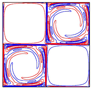
Figure 3. Streamlines of 2-D Taylor–Green vortices. $\varepsilon _e/\omega _{max}=0.2$. The solid (red) and dashed (blue) lines correspond to positive and negative values of the stream function, respectively. The contour levels are $\varPsi /\varPsi _{max} = \pm 0.16, 0.32, \ldots, 0.96$.

Scaling and the base-flow parameter have been chosen as in our previous work (Suzuki et al. Reference Suzuki, Hirota and Hattori2018; Hattori et al. Reference Hattori, Suzuki, Hirota and Khandelwal2021) for comparison purposes. Namely, the characteristic length has been set to the geometric mean of the rectangular cell $L_0=(L_xL_y)^{1/2}/2=1$, while the characteristic velocity has been chosen as

(4.3)\begin{equation} U_0 = \frac{\omega_{max}L_0}{2{\rm \pi}} = 1. \end{equation}

Two cases are considered: (i) $A=1$, which implies $L_x=L_y$ and $\varepsilon _e/\omega _{max}=0$, and (ii) $A=(7/3)^{1/4}$, which implies $L_x/L_y=\sqrt {7/3}$ and $\varepsilon _e/\omega _{max}=0.2$. Other choices of scaling are possible; for example, the Rossby number and the Froude number are divided by $2{\rm \pi}$ if we choose $\omega _{max}$, as the time scale as was done by Sipp et al. (Reference Sipp, Lauga and Jacquin1999).

4.2. Local stability analysis

The numerical method for local stability analysis is essentially the same as that of Suzuki et al. (Reference Suzuki, Hirota and Hattori2018) except that the Coriolis force is taken into account in the present work. Equations (2.15)–(2.18) were integrated in time by the fourth-order Runge–Kutta method. We consider periodic orbits of fluid particles throughout this paper. We also assume that the wavevector $\boldsymbol {k}$ is time-periodic which is a necessary condition for exponential instability on the periodic orbits. It is known that $\boldsymbol {k}$ is time-periodic if it is perpendicular to the streamline initially:

(4.4)\begin{equation} \boldsymbol{k}(0)\boldsymbol{\cdot}\boldsymbol{u}_b(\boldsymbol{X}(0))=0. \end{equation}

Then the time evolution of amplitude is described by a Floquet matrix $\boldsymbol{\mathsf{F}}$ since the matrices which appear in (2.17) is also time-periodic:

(4.5)\begin{equation} \{ \boldsymbol{a}, r\}(t+T)=\boldsymbol{\mathsf{F}}(T)\{ \boldsymbol{a}, r\}(t), \end{equation}

where $T$ is the period of $\boldsymbol {k}$ which coincides with that of the particle motion $\boldsymbol {X}$. Our task is to calculate the eigenvalues $\{ \mu _i \}$ of $\boldsymbol{\mathsf{F}}(T)$ which determines the growth rate as

(4.6)\begin{equation} \sigma_i=\frac{\log{|\mu_i|}}{T}. \end{equation}

Given the strength of rotation and stratification by the Rossby number $Ro$ and the Froude number $F_h$, the initial conditions should be specified to have particular solutions. Among the initial conditions, one parameter, which is denoted by $\beta$ in the following sections, is required for $\boldsymbol {X}(0)$ to identify a streamline in a 2-D flow. We set

(4.7)\begin{equation} \boldsymbol{X}(0)=\left(\frac{L_x}{4}(1-\beta), \frac{L_y}{4}, 0\right)^{\rm T}, \quad 0 \le \beta <1. \end{equation}

The elliptic stagnation point corresponds to $\beta =0$, while $\beta =1$ corresponds to the cell boundaries.

Another parameter is required for $\boldsymbol {k}(0)$ to specify the direction of the wavevector which satisfies (4.4); we take the angle between $\boldsymbol {e}_z$ and $\boldsymbol {k}(0)$, which is denoted by $\theta _0$. It should be pointed out that the magnitude of $\boldsymbol {k}(0)$ is arbitrary since the right-hand side of (2.17) depends only on the direction of $\boldsymbol {k}$ and is independent of the magnitude after taking the short-wave limit. For the amplitudes $\boldsymbol {a}(0)$ and $r(0)$, three independent initial conditions satisfying the incompressibility condition $\boldsymbol {a}(0)\boldsymbol {\cdot } \boldsymbol {k}(0)=0$ are considered; the results do not depend on the choice of the initial conditions since the space spanned by the three initial conditions is common. As a result, we obtain the largest growth rate $\sigma$ as a function of $\beta$, $\theta _0$, $Ro$ and $F_h$: $\sigma =\sigma (\beta, \theta _0, Ro, F_h)$.

4.3. Modal stability analysis

In the modal stability analysis, (2.9)–(2.11) were solved numerically by the Fourier spectral method (Peyret Reference Peyret2010) assuming periodic boundary conditions in all three directions, as was done by Hattori et al. (Reference Hattori, Suzuki, Hirota and Khandelwal2021). The time marching was performed by the fourth-order Runge–Kutta method.

Since the base flow is 2-D, the time evolution of disturbances is separable in the vertical direction. Thus, we set

(4.8)\begin{equation} \boldsymbol{u}' = {\rm e}^{{\rm{i}} k_z z} \sum_{k_x=-K_x}^{K_x}\sum_{k_y=-K_y}^{K_y} \tilde{\boldsymbol{u}}_{k_x,k_y} \exp({{\rm i} [k_x (x/L_x)+k_y (y/L_y)]}) \end{equation}

with similar expression for $p'$ and $\rho '$. The number of the Fourier modes is $500 \times 500$, the same as in the study by Hattori et al. (Reference Hattori, Suzuki, Hirota and Khandelwal2021).

The growth rate and frequency were obtained by the method of Krylov subspace (Edwards et al. Reference Edwards, Tuckerman, Friesner and Sorensen1994; Julien, Ortiz & Chomaz Reference Julien, Ortiz and Chomaz2004; Donnadieu et al. Reference Donnadieu, Ortiz, Chomaz and Billant2009; Hattori et al. Reference Hattori, Suzuki, Hirota and Khandelwal2021). Starting from randomized initial conditions, (2.9)–(2.11) were integrated for a certain long time. Intermediate states $\{(\pmb {u}'(T_0), \rho '(T_0)), (\pmb {u}'(T_0+\Delta T), \rho '(T_0+\Delta T)), \ldots, (\pmb {u}'(T_0+(N_K-1)\Delta T), \rho '(T_0+(N_K-1)\Delta T))\}$ were used as generators of the Krylov subspace. Then the eigenvalues and the eigenmodes were obtained in the $N_K$-dimensional Krylov subspace.

In this method, the error of an eigenvalue $\lambda$ of a linear operator $\boldsymbol{\mathsf{L}}$ can be evaluated by

(4.9)\begin{equation} \epsilon = \frac{\| {\boldsymbol{\mathsf{L}}}\boldsymbol{v}-\lambda\boldsymbol{v} \|}{\| \boldsymbol{v} \|}, \end{equation}

where $\boldsymbol {v}$ is the corresponding approximate eigenvector. The error $\epsilon$ depends on the initial time of the data $T_0$, the interval between the data $\Delta T$ and the dimension of the Krylov subspace $N_K$. To obtain eigenvalues accurately, several Krylov subspaces were generated from different sets of parameters and the eigenvalue with the smallest error for each eigenmode was chosen. The actual values of the parameters were chosen after trial and error. The number of data $N_K$ was fixed to $10$, the start time of the data was $T_0=195$ or $245$ and the interval between the data $\Delta T$ was fixed to $5$. Typically, the error of the eigenvalue is $\epsilon =O(10^{-10})$ for the largest eigenvalue for a fixed wavenumber $k_z$, while it increases for subdominant eigenmodes. In the following, we discarded the eigenmodes with $\epsilon \ge 10^{-3}$.

4.4. Realizability as a mode

As we see in § 5, the instabilities found by local stability analysis are not always found in modal stability analysis at finite Reynolds numbers since high-wavenumber modes are damped by viscous damping. In this case, the corresponding region of the instability in the $(\beta, \theta _0)$ plane is often thin so that it is difficult to construct an unstable mode. It is worth noting that Bayly (Reference Bayly1988) derived a condition for construction of an unstable eigenmode from local solutions of the form (2.12)–(2.14); the spatial width of the mode is approximately $[-\sigma ''(\beta )/2C(\beta )]^{-1/4}$, where $C(\beta )$ is an integral along a streamline and $C(\beta )>0$ is the condition since $\sigma ''(\beta )$ is normally negative. When $|\sigma ''(\beta )|$ is small, the unstable region in the local stability analysis is wide and the corresponding mode has a large spatial width; in other words, the radial wavenumber of the mode is small. Therefore, the eigenmode corresponding to a wider unstable region in the $(\beta, \theta _0)$ plane is less affected by viscous damping. Moreover, if the unstable region is wide in the $\theta _0$ direction, an eigenmode constructed by superposition of the local solutions can avoid viscous damping at lower Reynolds numbers.

With the above in mind, we intuitively introduce the following quantity:

(4.10)\begin{equation} \mathcal{R} = \int_{S} \sigma \sin\theta_0 \,{\rm d}\beta \,{\rm d}\theta_0, \end{equation}

where $S$ is the region of an instability on the $(\beta, \theta _0)$ plane, to quantify realizability as a mode of each instability; eigenmodes corresponding to an unstable region may not be found at finite Reynolds numbers and finite wavenumbers if $\mathcal {R}$ is small. It should be noted that existence of a mode depends on the Reynolds number; the critical Reynolds number at which a particular mode appears would increase as $\mathcal {R}$ decreases. In the above definition of realizability $\mathcal {R}$, the factor $\sin \theta _0$ is required to account for the solid angle since $\theta _0$ is the polar angle of a wavevector from the vertical axis in three dimensions. It should be pointed out that this is a crude approximation; for example, it would be better to replace $\theta _0$ by the average of $\theta$. However, it is sufficient to interpret the results of modal stability analysis since only the order of magnitude of $\mathcal {R}$ matters.