


1. Introduction
The impact of a liquid droplet on a solid surface is ubiquitous. It occurs in nature, industry and agriculture, such as raindrop impact on soil (Joung & Buie Reference Joung and Buie2015), inkjet printing (Derby Reference Derby2010) and pesticide deposition on plant leaves (Bergeron et al. Reference Bergeron, Bonn, Martin and Vovelle2000). During the impacting, droplets can spread, rebound or splash, depending on viscosity, surface tension, impact velocity and the properties of the solid surface (Josserand & Thoroddsen Reference Josserand and Thoroddsen2016). The maximum spreading of droplets is relevant to the inertia, surface tension and viscosity and, thus, involves two important dimensionless parameters: the Weber number  $We=\rho _H U_0^2 D_0/\sigma$ and the Reynolds number
  $Re=\rho _H U_0 D_0/\mu _H$, where
  $U_0$ is the initial impact velocity,
  $D_0$ is the initial droplet diameter,
  $\sigma$ is the surface tension coefficient,
  $\rho _H$ is the liquid density and
  $\mu _H$ is the dynamic viscosity.
At present, many theoretical models based on energy or momentum conservation have been proposed to predict the maximum spreading diameter ratio  $\beta _{max}=D_{max}/D_0$ of droplets impacting on a solid surface. In the literature, four scalings have been proposed to balance capillary, viscous and inertial forces. These include
  $\beta _{max} \sim Re^{1/4}$ (Pasandideh-Fard et al. Reference Pasandideh-Fard, Qiao, Chandra and Mostaghimi1996) and
  $\beta _{max} \sim Re^{1/5}$ (Roisman Reference Roisman2009; Wildeman et al. Reference Wildeman, Visser, Sun and Lohse2016) to balance viscous and inertial forces, and
  $\beta _{max} \sim We^{1/2}$ (Eggers et al. Reference Eggers, Fontelos, Josserand and Zaleski2010) and
  $\beta _{max} \sim We^{1/4}$ (Clanet et al. Reference Clanet, Béguin, Richard and Quéré2004) to balance capillary and inertial forces. However, the
  $We^{1/4}$ scaling may not be correct (Laan et al. Reference Laan, de Bruin, Bartolo, Josserand and Bonn2014) due to the balance being performed in a non-Galilean frame of reference in Clanet et al. (Reference Clanet, Béguin, Richard and Quéré2004). Laan et al. (Reference Laan, de Bruin, Bartolo, Josserand and Bonn2014) believed that all three forces play an important role when
  $We$ and
  $Re$ have similar values. They proposed a new scaling combining
  $Re^{1/5}$ and
  $We^{1/2}$, which is in good agreement with the experimental results. Besides, they found that the data points could not be collapsed onto one single curve using the scaling of
  $We^{1/4}$, suggesting that
  $We^{1/4}$ is not correct. Later, Lee et al. (Reference Lee, Laan, de Bruin, Skantzaris, Shahidzadeh, Derome, Carmeliet and Bonn2016) further took the wettability and roughness of solid surfaces into account, and proposed a universal rescaling of the
  $\beta _{max}$ for different liquids and surfaces. As for nanodroplets, the scaling laws of
  $\beta _{max} \sim We^{1/5}$ and
  $We^{2/3} Re^{-1/3}$ in low and high
  $We$ regimes, respectively, was proposed by Wang et al. (Reference Wang, Wang, He, Zhang, Yang, Wang and Lee2022).
The studies above are all about a droplet impacting on the rigid substrate, while there are few studies considering flexible substrates. According to previous studies, the flexible substrate also has a great influence on droplet impact. For superhydrophobic flexible substrates, Weisensee et al. (Reference Weisensee, Tian, Miljkovic and King2016) experimentally found that part of the momentum is returned to the droplet through the substrate's vertical vibration, resulting in a reduction of the contact time. Howland et al. (Reference Howland, Antkowiak, Castrejón-Pita, Howison, Oliver, Style and Castrejón-Pita2016) experimentally found that the energy consumption due to the deformation of the flexible substrate can reduce or suppress the splashing of droplets. While Pegg, Purvis & Korobkin (Reference Pegg, Purvis and Korobkin2018) found that the vibration of the flexible substrate is one of the key factors leading to splash through theoretical and numerical analysis. Vasileiou et al. (Reference Vasileiou, Gerber, Prautzsch, Schutzius and Poulikakos2016) experimentally found that the flexible substrate can enhance the superhydrophobicity of the solid surface, which is characterized by larger impalement resistance, smaller  $\beta _{max}$ and shorter contact time of droplet impact. Besides, this problem has been widely studied involving the raindrop impacting on biological surfaces (Gart et al. Reference Gart, Mates, Megaridis and Jung2015; Kim et al. Reference Kim, Wu, Esmaili, Dombroskie and Jung2020).
Although there are some qualitative experimental investigations, there are few quantitative analyses on the maximum spreading of droplets impacting flexible substrates. As far as we know, only Vasileiou et al. (Reference Vasileiou, Gerber, Prautzsch, Schutzius and Poulikakos2016) and Xiong, Huang & Lu (Reference Xiong, Huang and Lu2020) tried to perform quantitative analyses. However, Vasileiou et al. (Reference Vasileiou, Gerber, Prautzsch, Schutzius and Poulikakos2016) only considered the influence of the mass ratio of the droplet to the flexible plate, and the effect of the bending stiffness for plates was ignored. Xiong et al. (Reference Xiong, Huang and Lu2020) used the same methods as this work to perform relevant simulations. However, Xiong et al. (Reference Xiong, Huang and Lu2020) only focused on the two-dimensional (2-D) spreading dynamics in a very limited  $We$ range at a fixed mass ratio
  $M_r$. Furthermore, the final results were not normalized well.
In this paper a droplet impacting flexible plates over a wide range of  $We$ (0.1–100) in both two and three dimensions is simulated and quantitative analyses are carried out. Not only the effect of the stiffness
  $K_B$ of the flexible plate but also that of the mass ratio
  $M_r$ on the maximum spreading are investigated. Besides, the corresponding inherent mechanism is explored. We aim to seek a universal scaling law of
  $\beta _{max}$ in this flow problem.
2. Methodology and validation
A schematic diagram about a droplet impacting on a flexible plate is shown in figure 1(a). The droplet with a diameter  $D_0$ has a downwards impact velocity
  $U_0$. It is initially set above the centre of the flexible plate. The initial length of the plate is
  $L$ and the two ends of the plate are simply supported. Figure 1(b) shows the three-dimensional (3-D) viewpoint. Here, in our simulations, the phase-field lattice Boltzmann method (LBM) (Liang et al. Reference Liang, Xu, Chen, Wang, Chai and Shi2018) and the finite element method (Doyle Reference Doyle2001) are adopted for solving the fluid flow and the solid deformation, respectively. The conservative phase-field equation (Allen–Cahn equation) is used to track the fluid interface (Xiong et al. Reference Xiong, Huang and Lu2020)
 \begin{equation} \frac{\partial \phi}{\partial t}+\boldsymbol{\nabla} \boldsymbol{\cdot} (\phi \boldsymbol {u})=\boldsymbol{\nabla} \boldsymbol{\cdot} \left[M (\boldsymbol{\nabla} \phi-\frac{4}{\xi} \phi (1-\phi) \boldsymbol {\hat{n}}) \right], \end{equation}
where  $\phi$ is the component variable varying from 0 to 1, corresponding to light (vapour) and heavy (liquid) fluids, respectively. The densities of light and heavy fluids are
  $\rho _L$ and
  $\rho _H$, respectively. Here,
  $\boldsymbol {u}$ is the macroscopic velocity vector,
  $M$ is the mobility,
  $\xi$ is the interface thickness and
  $\boldsymbol {\hat {n}}$ is the unit vector normal to the fluid interface as
  $\boldsymbol {\nabla } \phi /\lvert \boldsymbol {\nabla } \phi \rvert$, pointing to the liquid. The isothermal, incompressible Navier–Stokes equation is solved by the LBM. The motion and deformation of the flexible plate for 2-D and 3-D cases are described by the structural equations (2.2) and (2.3), respectively (Hua, Zhu & Lu Reference Hua, Zhu and Lu2014; Xiong et al. Reference Xiong, Huang and Lu2020), i.e.
 $$\begin{gather} \rho_{s} h_s \frac{\partial^{2} \boldsymbol{X}}{\partial t^{2}}-\frac{\partial}{\partial s}\left[E h_s\left(1-\left|\frac{\partial \boldsymbol{X}} {\partial s}\right|^{{-}1}\right) \frac{\partial \boldsymbol{X}}{\partial s}\right]+E I \frac{\partial^{4} \boldsymbol{X}}{\partial^{4} s}=\boldsymbol{F}_{ext},\quad 2D,\end{gather}$$
 $$\begin{gather}\rho_{s}h_{s} \frac{\partial^{2} \boldsymbol{X}}{\partial t^{2}}-\sum _{i,j=1}^{2} \left[ \frac{\partial}{\partial s_i}\left(Eh_{s} \varphi_{ij}\left[\delta_{ij}-\left(\frac{\partial \boldsymbol{X}}{\partial s_i} \boldsymbol{\cdot} \frac{\partial \boldsymbol{X}} {\partial s_j}\right)^{{-}1/2} \right] \frac{\partial \boldsymbol{X}}{\partial s_j}- \frac{\partial}{\partial s_j} \left (E I \gamma_{ij} \frac{\partial^{2} \boldsymbol{X}}{\partial s_i \partial s_j} \right)\right) \right]\nonumber\\ =\boldsymbol{F}_{ext},\quad 3D, \end{gather}$$
where  $s$ is the Lagrangian coordinate along the plate direction,
  $\boldsymbol {X}$ is the position vector of the plate,
  $\rho _s$ is the plate density,
  $h_s$ is the plate thickness,
  $EI$ and
  $Eh_s$ are the bending and stretching stiffnesses, respectively, where
  $I=h_s^3/12$ and
  $E$ is Young's modulus. Here,
  $\varphi _{ij}$ and
  $\gamma _{ij}$ are the in-plane and out-of-plane effect matrices, respectively, and their components are
  $\varphi _{11}=\varphi _{22}=1$,
  $\varphi _{12}=\varphi _{21}=1/(2+2\nu )$,
  $\gamma _{11}=\gamma _{22}=1$ and
  $\gamma _{12}= \gamma _{21}=0$, where
  $\nu$ is Poisson's ratio. We denote by
  $\delta _{ij}$ the Kronecker delta function and
  $\boldsymbol F_{ext}$ the external force exerted by the fluid on the plate. The initial plate is straight, i.e.
  $(\partial ^2 \boldsymbol {X}^0 / \partial s_i^2 \boldsymbol {\cdot } \partial ^2 \boldsymbol {X}^0 / \partial s_j^2)^{1/2} = 0$ and the initial tension is zero, i.e.
  $(\partial \boldsymbol {X}^0 / \partial s_i \boldsymbol {\cdot } \partial \boldsymbol {X}^0 / \partial s_j)^{1/2} = \delta _{ij}$, where
  $\boldsymbol {X}^0$ is the initial position vector.

Figure 1. (a) The physical problem (two dimensional). (b) The three-dimensional (3-D) case. Here,  $W$ is the width of the plate.
Due to the symmetry of this problem, the following techniques are applied to save CPU time. In the 2-D cases, by applying a symmetric boundary condition, our computational domain is only half of the entire domain of the physical problem (see figure 2a). Similarly, for the 3-D cases, by applying the symmetric boundary conditions, our computational domain is only a quarter of the entire domain of the physical problem (see figure 2b). Here, the momentum exchange method is adopted for the moving boundary. Except for the symmetric boundaries, the outflow boundary conditions are applied for the other boundaries. As for the wettability of the substrate, the following Neumann boundary condition (Shao, Shu & Chew Reference Shao, Shu and Chew2013; Fakhari & Bolster Reference Fakhari and Bolster2017) is applied to impose the static contact angle:
 \begin{equation} \hat{n}_w \boldsymbol{\cdot} \boldsymbol{\nabla} \phi |_w = \varTheta \phi_w(1-\phi_w). \end{equation}
Here,  $\hat {n}_w$ is the unit vector normal to the solid boundary and
  $\phi _w$ is the component variable at the boundary point;
  $\varTheta$ is related to the equilibrium contact angle
  $\theta$, i.e.
  $\varTheta =-\sqrt {2\alpha /\kappa } cos \theta$, where
  $\alpha$ and
  $\kappa$ are related to the surface tension
  $\sigma$ and the interfacial thickness
  $\xi$ by
  $\alpha =12 \sigma / \xi$ and
  $\kappa =3 \sigma \xi /2$;
  $\phi _w$ and
  $\boldsymbol {\nabla } \phi |_w$ can be calculated from the values of
  $\phi$ in the surrounding nodes. To improve the accuracy, a weighted least squares method is adopted (Pan, Ni & Zhang Reference Pan, Ni and Zhang2018). More details about the implementation of this numerical method can be found in Xiong et al. (Reference Xiong, Huang and Lu2020).

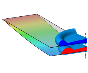
Figure 2. Snapshots of impacting droplets at the maximum spreading with  $We=60$ for rigid (blue) and flexible (red,
  $K_B=1.0$ and
  $M_r=0.01$) cases. In (a) the 2-D and (b) the 3-D cases, half and a quarter of the droplets are shown, respectively. Here,
  $d$ is the deflection of the plate at the centre. For the 3-D flexible case, on the plate, the contours of deflection in the
  $z$ direction are shown.
To make the above equations dimensionless, we choose  $\rho _H$,
  $D_0$ and
  $\sigma$ as characteristic quantities. The corresponding reference speed and time are
  $U_{ref}=\sqrt {\sigma /(\rho _H D_0)}$ and
  $T_{ref}=\sqrt {\rho _H D_0^3/\sigma }$, respectively. The key dimensionless parameters in the problem are the Weber number
  $We=\rho _H U_0^2 D_0/\sigma$, the bending stiffness
  $K_B=EI/(\rho _H U_{ref}^2 L^3)$ and the mass ratio
  $M_r=\rho _s h_s/(\rho _H L)$. Here, in our simulations, the density ratio is
  $\rho _H/\rho _L=1000$, the dynamic viscosity ratio
  $\mu _H/\mu _L=50$, the Ohnesorge number
  $Oh=\sqrt {We}/Re=0.01$, the contact angle
  $\theta =170^{\circ }$, the stretching stiffness
  $K_S=Eh_s/(\rho _H U_{ref}^2 L)=100$, the length ratio
  $L/D_0=20$ in 2-D cases, and
  $L/D_0=8$, the width ratio
  $W/D_0=3$ in 3-D cases. Because our numerical methods have been quantitatively validated in our previous work for the 2-D case (Xiong et al. Reference Xiong, Huang and Lu2020), here we mainly carried out validations for 3-D cases. The cases for droplets impacting on rigid substrates were simulated. Through the grid-independence study with different resolutions (
 $D_0=150\Delta {x}$,
  $300\Delta {x}$ and
  $600\Delta {x}$), we found that
  $D_0=300\Delta {x}$ is sufficient to obtain accurate results (not shown) and in the following simulations the resolution is adopted. In all of our 2-D and 3-D calculations, the computational domains are
  $10D_0\times 3D_0$ and
  $4D_0\times 1.5D_0\times 3D_0$ with a uniform Cartesian mesh, respectively.
Our numerical results, shown in figure 3(a), demonstrate good agreement with the universal rescaling of  $\beta _{max}$ proposed by Lee et al. (Reference Lee, Laan, de Bruin, Skantzaris, Shahidzadeh, Derome, Carmeliet and Bonn2016) for rigid cases. It is important to note that this rescaling depends not only on
  $We$ but also on
  $Re$. In line with this, all of our simulations were conducted with
  $Oh=\sqrt {We}/Re=0.01$, which means that
  $Re$ varied with
  $We$. Furthermore, our results for flexible cases also agree well with the numerical results of Dorschner et al. (Reference Dorschner, Chikatamarla and Karlin2018) in figure 3(b). Therefore, our numerical method for the simulations of a droplet impacting flexible plates is validated.

Figure 3. The  $\beta _{max}$ as a function of
  $We$ for (a) a rigid substrate, where the black squares represent our 3-D simulation results, and the solid line denotes the scaling of Lee et al. (Reference Lee, Laan, de Bruin, Skantzaris, Shahidzadeh, Derome, Carmeliet and Bonn2016). (b) Results for a flexible substrate, where the red and black symbols denote our results and those from Dorschner, Chikatamarla & Karlin (Reference Dorschner, Chikatamarla and Karlin2018), respectively.
3. Results and discussion
The droplet impacting on the flexible substrate would lead to a vertical movement of the substrate, which may affect the spreading of the droplet in turn. During this coupling process, the parameters, such as  $We$,
$We$,  $K_B$ and
  $M_r$, are all important. Here, we focus on their influences on the maximum spreading. A series of simulations in a wide range of parameters were performed, specifically,
  $We\in [0.1, 100]$,
  $K_B \in [0.01,\infty )$ and
  $M_r \in [0.006, \infty )$. It is noted that the cases of
  $K_B=\infty$ and
  $M_r=\infty$ correspond to the rigid case.
The results of the maximum spreading diameter ratio  $\beta _{max}$ as a function of
  $We$ are shown in figure 4. It can be seen from figure 4(a,c) that when
  $M_r$ is fixed, the maximum spreading
  $D_{max}$ is reduced as
  $K_B$ decreases at a specific
  $We$ in both 2-D and 3-D simulations. It can be simply described as ‘flexibility reduces spreading’. Similarly, when
  $K_B$ is fixed, the spreading is enhanced as
  $M_r$ increases. It can be understood as follows. When the inertia of the plate is relatively large (large
  $M_r$), it is hard to move and oscillate even if there is an impact from the droplet. The situation is similar to the rigid case. Therefore, the trend can be simply described as ‘inertia of plate enhances spreading’. A more detailed analysis about these can be seen in § 3.1.

Figure 4. The maximum spreading ratio  $\beta _{max}$ as a function of
  $We$ for cases with different
  $K_B$ but identical
  $M_r=0.01$ (a,c), and different
  $M_r$ but identical
  $K_B=0.6$ (b,d). (a,b) Two-dimensional cases. (c,d) Three-dimensional cases. The solid curves represent the universal rescalings of Lee et al. (Reference Lee, Laan, de Bruin, Skantzaris, Shahidzadeh, Derome, Carmeliet and Bonn2016) for rigid cases.
From figure 4 we can see that the trends of the simulation results for the 2-D and 3-D cases are similar. It can be understood in the following way. First, there is an inherent connection between the 2-D and 3-D substrate equations. The substrate equation for 3-D cases, i.e. (2.3), can degenerate into the 2-D equation, i.e. (2.2), if the spanwise length is infinite. Second, in both 2-D and 3-D cases, chordwise bending is dominant because only two chordwise ends of the plate are supported in the 3-D cases. Third, there is no spanwise bending and stretching of the plate in 2-D cases. The spanwise bending and stretching are also very minor in 3-D simulations because in the spanwise direction, i.e. the  $y$ direction in figure 1(b), both sides of the plate are free.
3.1. Evolutions of droplet spreading and energies
In order to understand the effect of the flexible substrate on droplet spreading, figure 5 shows snapshots of the impacting droplet at  $We=30$ and
  $M_r=0.01$ with four different
  $K_B$ values of 0.05, 0.6, 4.0 and
  $\infty$ (the rigid case). Once the droplet contacts the substrate (
 $t=0.04$), the flexible plate begins to move downwards. In all cases, all lamellas begin to move outwards. At
  $t=0.15$, we can see that there are rims in all cases. Besides, the more flexible the plate is, the smaller the spreading diameter. This indicates a lower averaged spreading speed in the case with a more flexible plate. However, in all cases the spreading diameters reach their peaks
  $D_{max}$ at approximately
  $t=0.45$. Hence, the flexible substrate has little effect on the maximum spreading time
  $t_{max}$ (
 $t \approx 0.45$), which is consistent with the observation in the experimental study of Vasileiou et al. (Reference Vasileiou, Gerber, Prautzsch, Schutzius and Poulikakos2016).

Figure 5. Snapshots of an impacting droplet for rigid and flexible cases (two dimensional) at  $We=30$,
  $M_r=0.01$ with different
  $K_B$: (a) rigid (
 $K_B=\infty$), (b)
  $K_B=4.0$, (c)
  $K_B=0.6$ and (d)
  $K_B=0.05$. Four typical moments (four columns)
  $t=0.04$, 0.15,
  $t_{max}$ and 0.7 are chosen. Here,
  $t_{max}$ is the moment when the maximum spreading occurs. The blue dotted lines denote the initial locations of the flexible plate. (d) Vertical deflection of the plate. In case (b), the spreading reaches
  $D_{max}$ after the plate's maximum deflection is achieved, namely, the delayed spreading case. In cases (c,d), the spreading reaches
  $D_{max}$ before that, namely, early spreading cases.
Here, we would like to discuss some details at  $t=t_{max}$. Figure 5 shows that at
  $t=t_{max}$ spreading reaches
  $D_{max}$ when the plate is moving downwards to its maximum deflection
  $d_{max}$ for small
  $K_B$, e.g. cases (c,d). These cases are referred to as ‘early spreading cases’. However, if
  $K_B$ is relatively large, e.g. case (b) with
  $K_B=4.0$, the oscillation frequency of the substrate is high enough, and upwards deflection of the substrate before
  $t_{max}$ may appear. It is referred to as the ‘delayed spreading case’ (see the caption of figure 5). In the delayed spreading case (figure 5b), a part of momentum or energy is returned to the droplet through the substrate's upwards motion, which results in a slight lifting up of the rim at the maximum spreading. This rising at
  $t=0.7$ is more obvious because the flexible substrate begins to move downwards again at this moment. The attached droplet also moves downwards, while the edge of the droplet still moves upwards, thus intensifying the rise of the rim. For cases (c,d) (
 $K_B=0.6$ and 0.05), because the flexible plate keeps a downwards movement during the droplet spreading, there is no rising rim.
Here, by the way, we would like to justify the parameter ranges in our study. From figure 5 we can see that in all cases any local segment of the plate is almost flat. This is the main characteristic of the cases that we investigated, i.e. the spreading of the droplet is not confined by the curvature effect of the plate. In this study we only focus on cases of this kind. On the other hand, when  $K_B$ and
  $M_r$ are small enough or
  $We$ is large enough, the impact on the flexible plate is more prominent. Furthermore, the local segment of the plate contacting the droplet may deform severely, which looks like a shallow well (see figure 6). Figure 6 shows a 2-D example with
  $K_B=0.01$,
  $M_r=0.01$ and
  $We=100$. In this case the rim of the well significantly confines the spreading of the droplet. Therefore, the flow regime would be significantly different from that in the present study. Since we are only interested in cases without confinement due to curvature, here we do not consider the cases with higher Weber numbers, i.e.
  $We>100$. For the same reason,
  $K_B<0.01$ and
  $M_r<0.006$ are not taken into account.

Figure 6. Local zoom-in view of a droplet impacting on the flexible plate with  $We = 100$,
  $K_B=0.01$ and
  $M_r = 0.01$ at
  $t=0.2$. The blue dotted line denotes the initial location of the flexible plate.
In the following, from the energy viewpoint, we explain why  $\beta _{max}$ decreases as
  $K_B$ or
  $M_r$ decreases as shown in figure 7. For the rigid case, the initial kinetic energy
  $E_k$ of the droplet is mainly converted into the surface energy at the maximum spreading. While, for flexible cases, part of the initial kinetic energy is converted into the elastic and kinetic energies of the plate, therefore, less energy is available for spreading, which results in a smaller
  $D_{max}$. Figure 7(a) shows the evolution of the spreading ratio
  $\beta$ and the total energy
  $E_t$ of the plate for cases in figure 5. We can see that at
  $t_{max}$ (
 $t\approx 0.45$),
  $E_t$ increases as
  $K_B$ decreases. Therefore, at
  $t_{max}$, more initial energy is transferred to the plate if it is more flexible. Besides, in the cases of different
  $M_r$ but fixed
  $K_B$ (see figure 7b), at
  $t_{max}$ (
 $t\approx 0.45$),
  $E_t$ increases as
  $M_r$ decreases. It is reasonable because if the plate is lighter (smaller
  $M_r$), the impact seems more significant, and more kinetic energy would pass to the plate. Therefore,
  $\beta _{max}$ decreases as
  $K_B$ or
  $M_r$ decreases, and is always smaller than rigid cases with the same
  $We$.
$We$.

Figure 7. The time evolution of  $\beta$ (solid lines) and the total energy of plates
  $E_t$ (dotted lines) for rigid and flexible cases at
  $We=30$ with (a) different
  $K_B$ (
 $M_r=0.01$ is fixed), (b) different
  $M_r$ (
 $K_B=0.6$ is fixed). The arrows point in the direction that
  $K_B$ or
  $M_r$ decreases. Here,
  $E_t$ contains the elastic and kinetic energies of the plate, which is zero for rigid cases.
In the analysis of energy conversion, the role of viscous dissipation should also be discussed. On the one hand, a more flexible substrate implies that more initial kinetic energy of the drop goes into the substrate. On the other hand, a more flexible substrate also suggests that the inertial shock during impact is mitigated. Consequently, the viscous dissipation inside the drop would decrease (due to smaller velocity gradients). This point is confirmed through our following tests. We carried out several simulations with  $We = 30$,
  $M_r=0.01$ but different
  $K_B$. The evolution of viscous dissipation and the total energy of substrates are shown in figure 8. We can see that the viscous dissipation decreases as the stiffness
  $K_B$ decreases.

Figure 8. The time evolution of viscous dissipation (solid lines) and the total energy of substrates (dotted lines are identical to those in figure 7a) in cases of  $We = 30$,
  $M_r=0.01$ but different
  $K_B$ (two dimensional). The viscous dissipation is calculated as
  $\mu _H (\partial u / \partial y)^2$ (Wildeman et al. Reference Wildeman, Visser, Sun and Lohse2016). The droplet reaches the maximum spreading at
  $t_{max}=0.45$.
Generally speaking, less viscous dissipation implies more surface energy of the droplet, which is favourable for droplet spreading. However, we can also see that when  $K_B$ changes, compared with the energy of the substrate, the viscous dissipation only changes in a very limited range and is minor. Therefore, the effect of viscous dissipation is very minor compared with the energy loss (absorbed by the substrates). Therefore, a more flexible substrate still leads to less surface energy (at
  $t_{max}$). The viscous dissipation does not affect the conclusion that the
  $\beta _{max}$ decreases as
  $K_B$ or
  $M_r$ decreases.
3.2. Rescaling the acceleration during impact
During impact, the droplet experiences a force exerted by the solid wall, which decelerates the droplet. According to Clanet et al. (Reference Clanet, Béguin, Richard and Quéré2004), the initial velocity  $U_0$ of the droplet decreases to
  $0$ at the maximum spreading along with a displacement of
  $D_0$ (rigid case in figure 2a) and, thus, the average acceleration
  $a$ during this process can be scaled as
  $a\sim U_0^2/D_0$. It is noted that Ye & Van Der Meer (Reference Ye and Van Der Meer2021) also got the same acceleration from the viewpoint of energy, considering this force being equal to the impact kinetic energy divided by the displacement. However, when the same droplet impacts the flexible substrate, its downwards movement leads to a larger displacement during the decelerating process as shown in figure 2. As a consequence, the average acceleration
  $a$ is reduced. It can be regarded that the droplet impacts the rigid surface with a lower initial velocity (Ye & Van Der Meer Reference Ye and Van Der Meer2021). We can understand this from figure 2 in which, for the flexible case, the droplet impacts the same surface as the rigid cases in a lower
  $We$, leading to a reduction of the maximum spreading diameter.
Vasileiou et al. (Reference Vasileiou, Gerber, Prautzsch, Schutzius and Poulikakos2016) scaled the average acceleration of droplets impacting on flexible substrates as
 \begin{equation} a \approx U_0^2/[D_0(1+m_d/m_b)], \end{equation}
considering the momentum conservation between the droplet and the substrate, where  $m_d$ and
  $m_b$ are their masses, respectively. It can only characterize the cases of different mass ratios but the stiffness effect is not considered. In other words, it is no longer applicable when
  $K_B$ changes.
However, as we have seen from our simulation results, the stiffness  $K_B$ can also significantly affect the maximum spreading. Moreover, Vasileiou et al. (Reference Vasileiou, Gerber, Prautzsch, Schutzius and Poulikakos2016) only considered the early spreading cases (small
  $K_B$, low vibration frequency) instead of the delayed spreading cases (large
  $K_B$), i.e. the spreading reaches
  $D_{max}$ after the plate's maximum deflection is achieved (see figure 5). Therefore, (3.1) is no longer applicable with a high
  $K_B$ or low
  $M_r$, which leads to a high vibration frequency in our simulation.
Here, we propose to rescale the average acceleration  $a$ for flexible substrates in the following way. As mentioned above, compared with the rigid case, the droplet impacting on flexible substrates travels a larger displacement during the deceleration process (see figure 2). Here, the total displacement scales as the sum of the initial droplet diameter and the maximum deflection of the flexible substrate, namely
  $D_0+d_{max}$. So the average acceleration can be rescaled as
 \begin{equation} a \sim U_0^2/(D_0+d_{max}), \end{equation}
where  $d_{max}$ contains the effects of both
  $K_B$ and
  $M_r$, as can be seen in (3.4).
In the following we would like to verify the rescaled average acceleration from the point of view of the energy. From the analysis above, we can see that compared with  $a \sim U_0^2/D_0$ for rigid cases, there is a smaller acceleration
  $a \sim U_0^2/(D_0+d_{max})$ in the flexible cases. We can imagine in terms of acceleration that the flexible case with velocity
  $U_0$ is equivalent to the rigid case with velocity
  $U_0 \sqrt {D_0/(D_0+d_{max})}$. Therefore, in the flexible case with
  $U_0$, the actual kinetic energy that is used for spreading to the maximum diameter is
  $E_{s, max} \approx E_k D_0/(D_0+d_{max})$, where
  $E_k$ is the initial kinetic energy. The remaining energy is supposed to be used for the deformation and motion of substrates, i.e.
  $E_{t, max} = E_k-E_{s, max} \approx E_k d_{max}/(D_0+d_{max})$, as discussed in § 3.1.
Figure 9(a) shows the total energy of the substrate at the maximum spreading  $E_{t,max}$ as a function of the initial kinetic energy
  $E_k$ for the cases with different
  $K_B$ or
  $M_r$. We can see that all the numerical data are below the black line
  $E_{t,max}=E_k$. This indicates that
  $E_{t,max}< E_k$, i.e. only part of
  $E_k$ is converted into
  $E_{t,max}$. To verify
  $E_{t, max}\approx E_k d_{max}/(D_0+d_{max})$, we change the coordinate of
  $E_k$ to
  $E_k d_{max}/(D_0+d_{max})$. The result is shown in figure 9(b), in which all the data points are around the black line, i.e.
  $E_{t, max}= E_k d_{max}/(D_0+d_{max})$. It is noted that even for the delayed spreading cases (
 $K_B=4.0$ and
  $1.0$ in figure 9), the results also agree well. Therefore, all of our data that come from cases with different
  $K_B$ or
  $M_r$ support the formula
  $E_{t, max}\approx E_k d_{max}/(D_0+d_{max})$. Since the formula is derived from (3.2), we confirm that all of our data support the rescaled acceleration.

Figure 9. The total energy of plates at the maximum spreading  $E_{t, max}$ as a function of (a) the initial kinetic energy
  $E_k$; and (b)
  $d_{max} E_k/(D_0+d_{max})$ for cases with different
  $K_B$ but a fixed
  $M_r=0.01$ (filled symbols), and those with different
  $M_r$ but a fixed
  $K_B=0.6$ (open symbols). The solid black lines denote
  $E_{t, max}=E_k$ and
  $E_{t, max}=d_{max} E_k/(D_0+d_{max})$ in (a,b), respectively. The colour of the symbols indicates the dimensionless maximum deflection of the plate
  $d_{max}/D_0$. Here,
  $E_{t,max}$ and
  $d_{max}$ are obtained through our numerical simulations (see the details of
  $E_{t,max}$ in figure 7).
3.3. Scaling law
In this section we aim to seek a nice data collapse by introducing an effective Weber number  $We_m$, which accounts for the substrate properties without any adjustable parameters. The aim is achieved by the energy analysis discussed in § 3.2. Furthermore, another effective Weber number
  $We_e$ directly derived from energy conservation confirms the validation of the scaling law.
From the above analysis, we know that in the flexible cases only a part of the kinetic energy (characterized by  $U_0^2$ or
  $We$) contributes to the spreading of the droplet. Here, an effective Weber number
  $We_m$ is defined to characterize the contribution. Since part of the initial kinetic energy,
  $E_k D_0/(D_0+d_{max})$ is available for spreading, we can define the effective Weber number as
 \begin{equation} We_m=\frac{We D_0}{D_0+d_{max}}=\frac{We}{1+\delta_{max}}, \end{equation}
where  $\delta _{max}=d_{max}/D_0$. To get the theoretical
  $We_m$, we have to theoretically determine
  $d_{max}$ first. Actually, the
  $d_{max}$ can also be obtained by the momentum conservation (Soto et al. Reference Soto, De Lariviere, Boutillon, Clanet and Quéré2014) as follows. The initial momentum
  $p_0$ of the droplet is
  $m U_0$, where
  $m$ is the mass of the droplet. After impact, the droplet and the flexible substrate vibrate together. According to Soto et al. (Reference Soto, De Lariviere, Boutillon, Clanet and Quéré2014), when the droplet impacts the flexible substrate, the centre of the substrate obtains a velocity
  $U_M=2{\rm \pi} f d_{max}$, where
  $f=f_0[M_s/(m+M_s)]^{1/2}$ is the vibration frequency of the system,
  $M_s$ the mass of the flexible substrate and
  $f_0$ the natural vibration frequency of the flexible substrate. For a simple-support plate on both ends, we have
  $f_0={\rm \pi} \sqrt {EI_M/M_sL^3}/2$ by the Euler–Bernoulli beam theory, where
  $I_M=h_s^3 W/12$ is the second moment of inertia (
 $W$ is the width of the plate and is set to unity in 2-D cases). Furthermore, according to Soto et al. (Reference Soto, De Lariviere, Boutillon, Clanet and Quéré2014), the plate vibrates with a parabolic shape and its momentum can be written as
  $p_M=2 \int _{0}^{L/2} \rho _s W h_s U_M x^2/L^2 \,{{\rm d} x} = M_sU_M/3$. Meanwhile, the momentum of the droplet vibrating at the centre of the substrate is
  $p_m=m U_M$. Due to momentum conservation, we have
  $p_0=p_M+p_m$. Therefore,
  $d_{max}$ can be predicted as
 \begin{equation} d_{max}=\frac{1}{2{\rm \pi}} \frac{m}{m+M_s/3} \frac{U_0}{f}. \end{equation}
 Figure 10 shows that the numerical results of  $\delta _{max}$ as a function of
  $We$ are in good agreement with the prediction of (3.4) for both 2-D and 3-D cases, which supports the above derivation.

Figure 10. The  $\delta _{max}$ as a function of
  $We$ for the (a) 2-D and (b) 3-D cases of different
  $K_B$ (
 $M_r=0.01$). The symbols represent the numerical results. The solid curve denotes the prediction of (3.4).
In the above, we can see that the effective Weber number  $We_m$ takes all the factors (
 $We$,
$We$,  $K_B$ and
  $M_r$) affecting
  $\beta _{max}$ into account. When
  $K_B$ or
  $M_r$ is large enough (close to the rigid case),
  $\delta _{max}\to 0$, we have
  $We_m \to We$. The theoretical
  $We_m$ values for all cases in figure 4 can be obtained through (3.3) and (3.4). Figure 11(a,b) shows the numerical 2-D and 3-D results of
  $\beta _{max}$ as a function of
  $We_m$, respectively. We can see that through
  $We_m$ all 2-D and 3-D data almost collapse onto a single curve, respectively. Furthermore, the single curve for 3-D cases can be well represented by the universal rescaling proposed by Lee et al. (Reference Lee, Laan, de Bruin, Skantzaris, Shahidzadeh, Derome, Carmeliet and Bonn2016).

Figure 11. The maximum spreading ratio  $\beta _{max}$ as a function of
  $We_m$ in the (a) 2-D and (b) 3-D cases, where all symbols come from figure 4. The solid line is the scaling of Lee et al. (Reference Lee, Laan, de Bruin, Skantzaris, Shahidzadeh, Derome, Carmeliet and Bonn2016) for rigid cases. (c) Original experimental data (
 $\beta _{max}$ as a function of
  $We$) for rigid and flexible cases in Vasileiou et al. (Reference Vasileiou, Gerber, Prautzsch, Schutzius and Poulikakos2016). (d) Plot of
  $\beta _{max}$ vs
  $We_m$ (data are identical to those in c). For black squares (rigid cases),
  $We_m=We$. For the red disks,
  $We_m=We/(1+m_d/m_b)$ (Vasileiou et al. Reference Vasileiou, Gerber, Prautzsch, Schutzius and Poulikakos2016). For the blue disks,
  $We_m$ is obtained through (3.3) and (3.4).
Besides our proposed scaling of (3.3), another similar scaling based on momentum conservation is available for different situations in the literature, i.e.  $We_m=We/(1+m_d/m_b)$ (Vasileiou et al. Reference Vasileiou, Gerber, Prautzsch, Schutzius and Poulikakos2016), where
  $m_d$ and
  $m_b$ are the masses of the droplet and plate, respectively. Figure 11(d) shows a comparison between different scalings. The blue and red symbols in figure 11(d) represent normalized data for flexible cases using our scaling of (3.3) and Vasileiou et al. (Reference Vasileiou, Gerber, Prautzsch, Schutzius and Poulikakos2016), respectively. The black symbols are normalized data for rigid cases, in which
  $We_m=We$. It is noted that the original data (Vasileiou et al. Reference Vasileiou, Gerber, Prautzsch, Schutzius and Poulikakos2016) are shown in figure 11(c). It is seen that through our scaling, all data collapse onto a single curve.
From figure 11(d) it can be seen that Vasileiou et al. (Reference Vasileiou, Gerber, Prautzsch, Schutzius and Poulikakos2016) can indeed correctly predict the maximum spreading diameter of the droplet impacting flexible substrates with the acceleration term of (3.1), even neglecting the change of the stiffness. However, this is attributed to the low natural frequency of flexible substrates, i.e. very flexible substrates. Since their substrates are very flexible, the assumption of a perfectly inelastic collision between the droplet and the substrates is valid. Under this assumption, they accurately obtained the initial velocity of the plate after impacting, then got the acceleration term correctly. Therefore, in their cases, they can neglect stiffness. However, when the stiffness is relatively large, the assumption of perfectly inelastic collision is no longer valid, and the acceleration term of (3.1) obtained by them is not applicable. While our derived acceleration is suitable for both large and small stiffnesses (figure 11a,b). Moreover, we can also get accurate theoretical predictions with the same stiffness as Vasileiou et al. (Reference Vasileiou, Gerber, Prautzsch, Schutzius and Poulikakos2016) (figure 11d).
In the following, we validate the scaling (3.3) through another effective Weber number  $We_e$, which is directly derived from energy conservation. From the analysis above, we know that for flexible substrates, the initial kinetic energy
  $E_k$ is converted into
  $E_s$ and
  $E_t$, i.e.
  $E_k = E_s + E_t$, and only
  $E_s$ contributes to the spreading. Suppose
  $We_e$ is proportional to the energy used for maximum spreading
  $E_{s,max}$, we have
 \begin{equation} We_e=We \frac{E_{s,max}}{E_k}=We\left(1-\frac{E_{t,max}}{E_k}\right). \end{equation}
On the other hand, from § 3.2 we know that  $E_{s,max} \approx E_k D_0/(D_0+d_{max})$. Substituting it into (3.5), we have
  $We_e \approx We D_0/(D_0+d_{max})$, which is almost identical to
  $We_m$. Although
  $We_e\approx We_m$, here
  $We_e$ (3.5) is a posteriori since
  $E_{t,max}$ has to be determined by numerical results, e.g. the data in figure 9. After
  $We_e$’s for all the cases in figure 4 are obtained, we can plot the maximum spreading ratio
  $\beta _{max}$ as a function of
  $We_e$ for all cases (see figure 12). We can see that all 2-D data almost collapse onto a single curve (figure 12a), so do the 3-D data (figure 12b). Furthermore, the single curve can also be well represented by the scaling of Lee et al. (Reference Lee, Laan, de Bruin, Skantzaris, Shahidzadeh, Derome, Carmeliet and Bonn2016).

Figure 12. The maximum spreading ratio  $\beta _{max}$ as a function of
  $We_e$ in the (a) 2-D and (b) 3-D cases, where all symbols come from figure 4. The solid line denotes the scaling of Lee et al. (Reference Lee, Laan, de Bruin, Skantzaris, Shahidzadeh, Derome, Carmeliet and Bonn2016) for rigid cases.
In summary, figures 11(b) and 12(b) show that  $We_m$ and
  $We_e$ formulas all lead to nice data collapses, which are all consistent with the scaling of Lee et al. (Reference Lee, Laan, de Bruin, Skantzaris, Shahidzadeh, Derome, Carmeliet and Bonn2016). It is noted that our proposed theoretical
  $We_m$ is a priori, and there are no adjustable parameters, while
  $We_e$ is a posteriori energy analysis that does confirm the validation of our a priori scaling law.
4. Conclusion
We have numerically simulated the droplet impacting on the flexible plate, and investigated the effect of the flexible substrate on the maximum spreading ratio  $\beta _{max}$ for different
  $K_B$ (
 $K_B\in [0.01,\infty )$) and
  $M_r$ (
 $M_r\in [0.006, \infty )$) in a wide range of
  $We$ (
 $We\in [0.1,100]$). Our study is limited to the cases in which droplet spreading is not affected by the substrate curvature. We observed that
  $\beta _{max}$ is reduced compared with the rigid case because partial initial energy is passed to the flexible plate, and less energy is available for spreading. Based on the energy analysis, we demonstrated that the vertical movement of the flexible substrate reduces the average acceleration
  $a$ during spreading, which can be regarded as the droplet impacting with less initial kinetic energy, leading to a decrease of the
  $D_{max}$. Furthermore, we theoretically derived an effective
  $We_m$, through which nice data collapses can be achieved. The scaling is also supported by an a posteriori energy analysis. Therefore, we successfully proposed a scaling of
  $\beta _{max}$ for droplets impacting flexible substrates (including the rigid cases) over a wide range of
  $We$.
$We$.
Funding
This work was supported by the National Science Foundation of China (NSFC) (grant nos. 11772326 and 11972342).
Declaration of interests
The authors report no conflict of interest.


