


1. Introduction
Turbulent Rayleigh–Bénard convection in confined volumes almost always leads to the formation of a large-scale circulation (LSC), sometimes called the ‘mean wind’, which, along with small-scale turbulent flows, provides transport of heat and various passive scalars (Ahlers, Grossmann & Lohse Reference Ahlers, Grossmann and Lohse2009; Chillà & Schumacher Reference Chillà and Schumacher2012; Xia Reference Xia2013). Of interest are both the dynamics of LSC, which can be rather complex, and the ways to control it. There are a number of ways of controlling large-scale flows, such as spatial variation of temperature boundary conditions (Wang, Huang & Xia Reference Wang, Huang and Xia2017; Bakhuis et al. Reference Bakhuis, Ostilla-Mónico, van der Poel, Verzicco and Lohse2018; Nandukumar et al. Reference Nandukumar, Chakraborty, Verma and Lakkaraju2019; Vasiliev & Sukhanovskii Reference Vasiliev and Sukhanovskii2021; Sukhanovskii & Vasiliev Reference Sukhanovskii and Vasiliev2022), changes in surface roughness (Toppaladoddi, Succi & Wettlaufer Reference Toppaladoddi, Succi and Wettlaufer2017; Xie & Xia Reference Xie and Xia2017; Zhu et al. Reference Zhu, Stevens, Verzicco and Lohse2017; Jiang et al. Reference Jiang, Zhu, Mathai, Verzicco, Lohse and Sun2018; Zhang et al. Reference Zhang, Sun, Bao and Zhou2018; Zhu et al. Reference Zhu, Verschoof, Bakhuis, Huisman, Verzicco, Sun and Lohse2018) and vertical or horizontal baffles (Ciliberto, Cioni & Laroche Reference Ciliberto, Cioni and Laroche1996; Bao et al. Reference Bao, Chen, Liu, She, Zhang and Zhou2015; Vasiliev, Sukhanovskii & Frick Reference Vasiliev, Sukhanovskii and Frick2022). Another promising approach is to introduce freely moving immersed bodies with one or more degrees of freedom into the fluid volume. The application of this approach requires an understanding of the dynamics of turbulent convective systems with moving submerged bodies of finite size, which, on the one hand, are entrained by the flow, and on the other hand, directly affect the heat and mass transfer. A recent paper of Wang & Zhang (Reference Wang and Zhang2023) shows that vertical freely rotating baffle results in a remarkable and rather unexpected transformation of the LSC in Rayleigh–Bénard convection in the cylindrical container.
Obviously, in the general case of arbitrary cavity geometry, shape and properties of the floating body, a great diversity of the system behaviour is possible. To elucidate at least the basic regularities of the behaviour of the system, which includes a convective cell and a free-floating body, it is necessary to identify some simplified (academic) problems. As such a problem, we can take Rayleigh–Bénard convection (horizontal layer, heated from below and cooled from above) with a plate floating only along the horizontal.
A plate floating on the free surface of a fluid layer heated from below is a particular case of this problem originating from the convective scenario of tectonic plate drift (Schubert, Turcotte & Olson Reference Schubert, Turcotte and Olson2001). The first experiments of Elder (Reference Elder1967) showed that a floating plate on the free surface is not a passive drifter and can move without preexisting streams. Later, this problem has been studied experimentally (Zhang & Libchaber Reference Zhang and Libchaber2000; Zhong & Zhang Reference Zhong and Zhang2005, Reference Zhong and Zhang2007a), numerically (Gurnis Reference Gurnis1988; Zhong & Gurnis Reference Zhong and Gurnis1993; Whitehead & Behn Reference Whitehead and Behn2015; Mao, Zhong & Zhang Reference Mao, Zhong and Zhang2019; Mao Reference Mao2021) and theoretically (Mac Huang et al. Reference Mac Huang, Zhong, Zhang and Mertz2018). These studies showed that interaction between the plate and the fluid flow may result in periodic and irregular plate drifts, depending on the plate size and Rayleigh number. It should be noted that numerical simulations were done using an infinite Prandtl number for a better approximation of mantle convection.
Modelling of tectonic plate drift is an interesting but a particular case of the system, which includes a convective layer and a free floating body. There are many configurations in which a floating body of different nature can block the vertical heat flux. One can mention convective envelopes of stars (e.g. the Sun), where a localized magnetic field damps the motions of the conducting medium, but is entrained by the moving conducting medium, so this band may be regarded as a floating obstacle for convective heat fluxes, which can affect the formation of large-scale flows in the pole-equator direction. The cloud clusters in the Earth atmosphere play an important role in radiative heat exchange. The formation of an oil lens following large-scale oil spills can also be viewed as a floating body, and estimating its drift requires an understanding of the interaction between an oil lens and the surrounding fluid. In industrial applications, solid phase clusters can also have a strong influence on non-isothermal chemical reactions, metallurgical and crystallization processes. In the present study, we focus on some general properties of a free-floating body inside a convective layer in a rather simple academic formulation (Popova & Frik Reference Popova and Frik2003). In such a system, the character of body motion and the structure of the flow significantly depend on the Rayleigh number, the geometry of the cell and the vertical location of the plate. Regular, periodic motions of the body from one edge of the cell to the other were observed in the limited range of governing parameters. Changes in the distance between the plate and the isothermal boundary, the length of the cell and the heating rate lead to significant changes in the dynamics of the floating body. Transient regimes, in which periodic oscillations occur irregularly, and chaotic regimes, in which there are no intervals of regular oscillations, were observed. In addition to changes in the flow structure, the insulating body inside the fluid can significantly affect the heat transfer (Popova et al. Reference Popova, Vasiliev, Sukhanovskii and Frick2022; Vasiliev et al. Reference Vasiliev, Sukhanovskii and Frick2022; Filimonov et al. Reference Filimonov, Gavrilov, Dekterev and Litvintsev2023). The variation of each particular parameter can have a strong influence on the flow structure and immersed plate dynamics. Therefore, a more systematic approach is required to better understand the role of the main parameters.
The goal of this study is to reveal the specific features of the complex system consisting of Rayleigh–Bénard convection and an immersed floating plate. The most attention is paid to the plate drift dynamics, structural changes in the flow and variation of heat transfer.
The structure of the paper is as follows. The statement of the problem and governing parameters are given in § 2. The experimental set-up and mathematical model are described in § 3. The main results, including description of the periodic regime, so-called convective pendulum (§ 4.1) and more complex non-periodic regimes, provided by variation of aspect ratios (§ 4.2), immersion depth (§ 4.3) and Rayleigh number (§ 4.4), are presented in § 4. The influence of the immersed body motion on heat transfer is described in § 4.5. A summary and conclusions are given in § 5.
2. Statement of the problem and governing parameters
In the present study, we consider Rayleigh–Bénard convection in a closed cell with a free-floating body held in a fixed vertical position. The floating body has one degree of freedom and can move only along horizontal coordinate  $x$ (figure 1). At the boundaries of the body, the no-slip and adiabatic conditions are fulfilled. The upper and lower boundaries of the cell are kept at constant temperatures
  $T_c$ and
  $T_h$, and the sidewalls are adiabatic. All solid boundaries satisfy the non-slip condition.

Figure 1. Schematic diagram of Rayleigh–Bénard convection in a closed cell with a free-floating body.
Thermal convection is governed by the following non-dimensional parameters: the Rayleigh number  $\textit {Ra}$, which is the ratio of buoyancy to dissipative forces, and the Prandtl number
  $\textit {Pr}$, which is the ratio of kinematic viscosity
  $\nu$ to thermal diffusivity
  $\chi$
 \begin{equation} \textit{Ra}=(g\alpha \Delta T H_1^{3} )/(\nu \chi ), \quad \textit{Pr}=\nu/\chi, \end{equation}
where  $\Delta T=T_{h}-T_{c}$ is the temperature drop between the lower and upper boundary,
  $g$ is the gravity acceleration,
  $\alpha$ is the thermal expansion coefficient and
  $H_1$ is the layer height. All experiments were performed with water at the average temperature
  $T_0=22^\circ {\rm C}$ at which the Prandtl number
  $\textit {Pr}=6.6$. The simulations were performed for the same value of the Prandtl number.
When considering convection in a finite volume of fluid, it is necessary that geometrical parameters be added to the control parameters. In the classical Rayleigh–Bénard problem, the main geometric parameter is the ratio of the horizontal size of the cavity to the vertical size. In problems with fixed inclusions (Cooper, Moresi & Lenardic Reference Cooper, Moresi and Lenardic2013; Wang et al. Reference Wang, Huang and Xia2017; Vasiliev et al. Reference Vasiliev, Sukhanovskii and Frick2022) or free-floating bodies (Zhang & Libchaber Reference Zhang and Libchaber2000; Popova & Frik Reference Popova and Frik2003; Zhong & Zhang Reference Zhong and Zhang2005, Reference Zhong and Zhang2007a,Reference Zhong and Zhangb; Mao et al. Reference Mao, Zhong and Zhang2019; Mao Reference Mao2021), additional parameters are introduced to determine the global structure of the flow and the heat and momentum transfer. In our case, the problem includes three geometric parameters: two aspect ratios that characterize the relative cavity extent and the relative horizontal dimensions of the floating body, as well as the relative height of the body location:
 \begin{equation} \varGamma_{1}=L_{1}/H_{1}, \quad \varGamma_{2}=L_{1}/D, \quad d=h/H_{1}, \end{equation}
where  $L_1$ is the layer length,
  $D$ is the plate size, and
  $h$ is the distance between the plate and the bottom (see table 1).
Table 1. Governing parameters in numerical and experimental runs.

The main response characteristics of the convective flow are the global heat and momentum transport represented by the dimensionless Nusselt number  $\textit {Nu}$ and Reynolds number
  $\textit {Re}$, respectively. Within the Oberbeck–Boussinesq approximation, the Nusselt number is
 \begin{equation} {\textit{Nu}=\frac{H_1}{\Delta T}\left\langle \left.\dfrac{\partial T}{\partial y}\right|_{y=0} \right\rangle_{x,t}}, \end{equation}
where  $\langle {\cdot } \rangle _{x,t}$ denotes averaging over time and over coordinate
  $x$.
$x$.
For the Reynolds number, we use the definition which is based on the mean square root of the fluid velocity,
 \begin{equation} {\textit{Re} = \frac{H_{1}\sqrt{\langle{\boldsymbol u}\boldsymbol{\cdot}{\boldsymbol u}\rangle_{t,V}}}{\nu}}, \end{equation}
where  $\langle {\cdot } \rangle _{t,V}$ denotes averaging over time and over the entire convection cell.
In a convective cell with a free-floating body, oscillatory modes arise at a certain combination of control parameters. Then the natural dimensionless characteristic of the body motions is the Strouhal number, which is defined as the body oscillation frequency  $f$ measured in convective flow units,
  $\textit {St}=f L_1/V$. In other words, the Strouhal number is the ratio of the characteristic velocity of the solid body (
 $U=L_{1}/\tau _{0}$) to the convective velocity (the free-fall velocity
  $u_{f}=\sqrt {g\alpha \Delta T H_{1}}$):
 \begin{equation} \textit{St} = \frac{U}{u_{f}}=\frac{L_{1}}{\tau_{o} \sqrt{g\alpha \Delta T H_{1}}}. \end{equation}
3. Methods
3.1. Experiment
The experimental set-up is a parallelepiped of length  $L=500$ mm, width
  $W=100$ mm and height
  $H=180$ mm (figure 2). The side walls are made of 10 mm thick transparent Plexiglas. The top and bottom plates are made of copper and act as heat exchangers.

Figure 2. Experimental set-up: 1, lower heat exchanger; 2, upper heat exchanger; 3, inlets and outlets of upper heat exchanger; 4, holders of upper heat exchanger; 5, cell walls (Plexiglas); 6, frame; 7, supporting rods; 8, slot of upper heat exchanger; 9, free-floating disk; 10, Plexiglas baffles.
The upper heat exchanger, which is 27 mm thick, is cooled by circulating thermostatically controlled ethylene glycol. The channels in the heat exchanger are designed so that the inlet and outlet are adjacent to each other to ensure uniform temperature boundary conditions. In the middle of the plate, there is a 5 mm wide longitudinal slot to allow free movement of the rod that controls the immersion of the thermal insulating body.
The lower heat exchanger, which is 10 mm thick, is heated with a silicone heater glued to the underside. The experiments were performed at constant temperature at both boundaries. The temperature of the bottom heat exchanger was controlled using a proportional–integral–derivative controller with an accuracy of 0.1 $^{\circ }$C. The maximum heating power was 150 W. Calibrated copper-constantan thermocouples were used to record the temperature of the upper and lower heat exchangers. In the lower heat exchanger, one thermocouple was located at the periphery (50 mm from the edge) and the other was located in the central part. In the upper heat exchanger, two thermocouples were located at different edges of the copper plate. Temperature and power measurements were recorded with a measuring board (at a frequency of 1 Hz).
Distilled water was used as the working fluid, the level of which was approximately 20 mm above the upper heat exchanger. The free-floating body was a 1 mm thick Plexiglas disk with a diameter of  $D=98$ mm, which is slightly smaller than the width of the layer. The body was submerged to a given depth by means of a thin rod which was fixed at the centre of the disk and had a float attached to its upper end. Note that a series of experiments with a body floating on a free surface (Zhang & Libchaber Reference Zhang and Libchaber2000; Zhong & Zhang Reference Zhong and Zhang2005, Reference Zhong and Zhang2007a,Reference Zhong and Zhangb) were performed using rectangular plates of hydrophobic material, which allowed avoiding its contact with the model walls. In the experiment with an immersed body, it is impossible to avoid touching the wall, which causes the rotation of the body about the vertical axis and braking. The disc shape of the body allows one to minimize the interaction between the floating body and the model walls, which was successfully demonstrated by Popova & Frik (Reference Popova and Frik2003).
The free-floating body movements were registered with a time interval of 6 s using a Bobcat B2020 CCD camera. The position of the body was determined by the location of the thin rod attached to the centre of the disk. The duration of the experiments varied from 6 to 24 h.
An important difference between our set-up and the one described by Popova & Frik (Reference Popova and Frik2003) is the possibility of changing the geometric parameters of the cell. For this purpose, two vertical Plexiglas baffles 5 mm thick were placed inside the cell, which bound the working cavity of length  $L_{1}$. By varying the position of the baffles and the distance between the heat exchangers, we can be vary
  $L_{1}$ and
  $H_{1}$ within a fairly wide range. In the experiments described below, the width and height of the layer were fixed (
 $W=100$ mm,
  $H_{1}=40$ mm), and
  $L_{1}$ varied from 112 to 500 mm.
3.2. Numerical simulations
A full understanding of the behaviour of the complex system, which includes an extended floating immersed body and Rayleigh–Bénard convection, requires knowledge of the structure of the flow and temperature field, as well as the distribution of temperature and viscous stresses at the body surface. It is a bit of a challenge to get all these characteristics experimentally, so that in addition to experiments, we perform a series of numerical simulations in a setting very close to the experimental one. Direct three-dimensional (3-D) numerical simulations for the developed convective flows demand significant computational resources and are not suitable for our purposes as we intend to vary the main control parameters. Therefore, we limited ourselves to two-dimensional (2-D) numerical simulations.
Numerical simulations were performed within the framework of a two-dimensional model which includes the equations of free convection of incompressible fluid in an Oberbeck–Boussinesq approximation and the equation of motion of the solid plate. The unsteady fluid flow is described by the Navier–Stokes equation, which includes the buoyancy force, the temperature equation and the continuity equation:
 \begin{gather} \frac{\partial \boldsymbol{u}}{\partial t} +(\boldsymbol{u}\boldsymbol{\cdot} \boldsymbol{\nabla} )\boldsymbol{u}={-}\frac{\boldsymbol{\nabla} p}{\rho } +\nu \nabla ^{2} \boldsymbol{u}- \boldsymbol{g}\alpha (T-T_{0} ), \end{gather}
 \begin{gather}\frac{\partial T}{\partial t} +(\boldsymbol{u}\boldsymbol{\cdot} \boldsymbol{\nabla} )T=\chi \nabla ^{2} T, \end{gather}
 \begin{gather}\boldsymbol{\nabla} \boldsymbol{\cdot} \boldsymbol{u} = 0. \end{gather}
Here,  $\boldsymbol {u}=(u_x,u_y)$ denotes the velocity vector field,
  $x$ is the horizontal coordinate,
  $y$ is the vertical coordinate,
  $\rho$ is the density,
  $T$ is the temperature,
  $T_0$ is the reference temperature and
  $p$ is the pressure.
The motion of the solid plate is described by Newton's equation:
 \begin{equation} \frac{{\rm d} V}{{\rm d} t} = \frac{(\boldsymbol{f}_p+\boldsymbol{f}_\nu)_x}{m}, \end{equation}
where  $V$ is the plate velocity, which is purely horizontal,
  $\boldsymbol {f}_p$ and
  $\boldsymbol {f}_\nu$ are the pressure and viscous forces, and
  $m$ is the mass of the plate. The forces are calculated by the integration over the plate surface,
 \begin{equation} \boldsymbol{f}_p=\oint p \boldsymbol{n} \,{\rm d}S, \quad \boldsymbol{f}_\nu={-}\oint \boldsymbol{\tau}_w \,{\rm d}S, \end{equation}
where  $\boldsymbol {\tau }_w$ is the viscous wall stress. The impact of the plate into the wall is considered inelastic. The model of the solid plate motion in the fluid is implemented using the immersed boundary method (Mittal & Iaccarino Reference Mittal and Iaccarino2005). A detailed description of the mathematical model and results of its testing are presented by Filimonov et al. (Reference Filimonov, Gavrilov, Dekterev and Litvintsev2023).
At all solid boundaries (including both plate surfaces), no-slip conditions are set for the velocity. The upper and lower boundaries are held at fixed temperatures. The lateral boundaries and boundaries of the plate are adiabatic. At the initial moment of time, the fluid velocity in the computational domain is zero, and the temperature is the arithmetic mean of the upper and lower boundary temperature. The plate is located in the centre of the cell ( $x_{0}=0$).
Numerical calculations were performed with the in-house CFD code  $\sigma$ Flow, the numerical algorithm of which is based on the unstructured spatial grid and finite volume method for hydrodynamic equations.
The approximation of convective and diffusive terms of the equation of motion is carried using the second-order central difference schemes. The relationship between the velocity and pressure fields, providing the fulfilment of the continuity equation, is realized using a SIMPLE-like splitting procedure. To integrate the equation of motion in time, the Crank–Nicholson method of second-order accuracy is used. Both viscous and convective terms of the equation of motion are treated implicitly. The convective terms of the energy transfer equation are approximated by the second-order upwind TVD scheme, and the unsteady term of the temperature equation is approximated by the second-order three-layer scheme. An algebraic multigrid method is used to solve the linear system resulting from the discretization of the pressure correction equation. To speed up calculations, we use the parallel computation technology based on decomposition of the computational domain into several adjoining subdomains.
The simplicity of the geometry and the use of the immersed boundary method to describe the motion of the solid plate allows the application of a structured computational grid.
A mesh independence study was performed by varying the cell size of the mesh and examining the integral parameters. Verification calculations were performed for flow at  $\varGamma _2=1.73$,
  $\textit {Ra}=10^7$ and
  $d=0.1$. Using the numerical solution on three different meshes with cell sizes coarse 0.5 mm, base 0.25 mm and fine 0.125 mm, we performed the procedure of estimation of grid convergence and discretization error (Celik et al. Reference Celik, Ghia, Roache and Freitas2008). The following integral parameters were chosen for the estimation: heat flux, mean kinetic energy and mean viscous dissipation rate of kinetic energy. The grid convergence index, GCI, for the fine mesh with factor of safety of three and formal second-order accuracy does not exceed
  $2\,\%$. The GCI values for the base mesh remain within
  $5\,\%$. The results confirm that the numerical accuracy of the modelling with the base mesh is within acceptable limits for CFD modelling (see table 2). During numerical simulation, the time integration step remained constant and was chosen to be 0.03 s. The maximum Courant–Friedrichs–Levy number did not exceed unity and the average value over the whole region was
  $0.32 \pm 0.25$. The average simulation time was at least 3000 s of physical time. Then the results of the described mathematical model of two-dimensional Rayleigh–Bénard convection modelling were cross-verified with the results of modelling performed by van der Poel et al. (Reference van der Poel, Stevens, Sugiyama and Lohse2012). For this purpose, three calculations for
  $\textit {Ra}=10^8$ with different aspect ratios of the computational domain were performed:
  $\varGamma _1 = 4.25$, 4.9 and 10.3. Obtained results are in a very good agreement with van der Poel et al. (Reference van der Poel, Stevens, Sugiyama and Lohse2012). In the first two configurations, the flow with three large scale rolls in the computational domain was established, and for the third configuration with seven rolls. The deviation in the Nusselt number between the results of our calculations and numerical results (van der Poel et al. Reference van der Poel, Stevens, Sugiyama and Lohse2012) does not exceed
  $2\,\%$.
Table 2. Nusselt number  $\textit {Nu}$, Reynolds number
  $\textit {Re}$ and Strouhal number
  $\textit {St}$ calculated for different Rayleigh number using different grids (at
  $\textit {Ra} = 8\times 10^{7}$, the plate motion is aperiodic).

4. Results
4.1. Convective pendulum
We will begin the description of the results with consideration of the basic mode, in which the plate executes periodic motions from one wall to another – the convective pendulum mode. Such a pendulum mode was observed earlier both when the rectangular plate was floating on the surface (Zhang & Libchaber Reference Zhang and Libchaber2000) and when the disk was floating near the bottom (Popova & Frik Reference Popova and Frik2003). The mechanism of periodic motion of the plate in this mode is as follows. The plate, being close to one of the walls, blocks the vertical heat flow, and in the gap at the opposite wall, an intense upward flow is formed. It promotes the development of a large-scale flow, which entrains the plate and carries it to the opposite wall, after which all events are repeated in reverse sequence. The experiments of Popova & Frik (Reference Popova and Frik2003) have shown that in a relatively short cavity ( $4.25 < \varGamma _1< 8.50$,
  $\varGamma _2=1.70$), stable periodic motions are realized in the whole range of the Rayleigh numbers considered but only at a sufficiently low position of the disk (
 $d\lesssim 0.15$). As the distance between the disk and the bottom increases, the periodicity begins to break down. The details of this process will be described below.
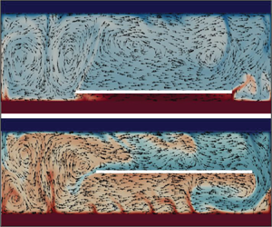
To illustrate the mechanism of convective pendulum, we present a set of velocity fields obtained by 2-D numerical simulations for the layer of depth  $H=40$ mm, the plate located at a height of
  $h=4$ mm (
 $d= 0.1$), the Rayleigh number
  $\textit {Ra} = 8.6\times 10^6$, and the aspect ratios
  $\varGamma _1= 3.06$ and
  $\varGamma _2= 1.25$. Figure 3 shows the individual phases of the ‘pendulum’ motion. Figure 3(a) corresponds to the instant of time when the plate passes the centre of the layer, moving to the right. It is ‘pulled’ by an intense vortex located at the right wall. Figure 3(b) shows the time when the plate is already in contact with the right wall and an intense vortex of the opposite sign is spinning at the left wall. Figure 3(c) shows the time of plate ‘departure’ from the right wall. It is pulled by the vortex at the left wall, which begins to grow at this stage, reaching the size of half of the cell by the time the plate passes the centre of the cell (figure 3d). In figure 3(e), the plate is pressed against the left wall and a new vortex begins to develop in the vacated heated space on the right side, drawing the plate towards itself. The change in the flow structure during the plate movement is characterized by significant changes in the total kinetic energy of the fluid (see figure 3f, which shows changes in the plate position and kinetic energy during one cycle and indicates the time instants at which the velocity fields are depicted). The time dependence of the kinetic energy
  $E_k$ shows that there is a sharp rise in
  $E_k$ as the plate is parked near one of the walls. The mechanism of such sharp pulsations of kinetic energy is due to the fact that the liquid under the plate is strongly overheated. Its potential energy increases, which inevitably leads to instability with the result that a heated jet of liquid breaks forth from under the plate, forming an intense vortex (figure 3b). Then, as is seen in figure 3(c), this vortex grows, losing its intensity, and after reaching a certain size, it carries the plate to the opposite wall.

Figure 3. Instantaneous velocity fields at (a)–(e) five time moments, indicated in panel (f), where the variations of the plate position (blue line) and total kinetic energy of the fluid (red line) are shown for one period of the convective pendulum. Numerical simulations for  $\varGamma _1= 3.06$,
  $\varGamma _2=1.25$,
  $\textit {Ra} = 8.6\times 10^6$ and
  $d=0.1$. Black arrows under the corresponding panels indicate the plate velocity.
As noted above, the convective pendulum occurs in a limited domain of control parameters, beyond which the disturbances of the periodic regime are observed. The identification of the domain, in which the convective pendulum exists, and investigation of possible scenarios of periodic mode failure is a complex and time-consuming problem. This is due to the fact that, despite the apparent simplicity of the system, there is a set of parameters which have a significant influence on the structure and dynamics of the convective flow and, as a consequence, on the plate motion. First of all, it is the geometry of the layer determined by the aspect ratio  $\varGamma _1$. At large values of
  $\varGamma _1$ (horizontally stretched layer), a convective flow usually represents a set of convective cells, the size of which is comparable to the layer thickness. At
  $\varGamma _1\sim 1$, it is a single cell, and in the case of vertically stretched layer, at small values of
  $\varGamma _1$, the convective flow can be formed by a single-cell structure stretched in the vertical direction or by a set of cells located one above the other. The aspect ratio
  $\varGamma _2$ determines the degree of influence of the immersed body on the flow; with increase of
  $\varGamma _2$, the influence of the body on the structure of convective flows decreases.
Another important parameter is the depth of the plate immersion (relative distance from the plate to the bottom  $d$). In the case of small
  $d$, when the body is located near the temperature boundary layer, there is a noticeable decrease in the heat flux under it, and the main convective flow is located above the body. When the body is located closer to the middle of the layer, the formation of competing convective cells located above and below the body is observed. All the above processes depend on the convection intensity determined by the Rayleigh number and the fluid properties determined by the Prandtl number. The shape and properties of the immersed body, in addition to its size and position in the layer, can also affect the system. The conducted experiments revealed a number of additional factors, which are related to the specific realization of the floating body and conditions at the boundaries. Due to a large number of parameters, a detailed study of the described system requires significant efforts. In the following, we demonstrate possible scenarios of the evolution of the convective pendulum associated with the variations in the main parameters.
4.2. Variation of aspect ratios  $\varGamma _{1}$ and $\varGamma _{2}$


First, let us show how the convective pendulum is affected by a change in the layer length at fixed values of the plate size and height (both aspect ratios are changed). To do this, we set the plate in the layer of depth  $H=40$ mm at a height
  $h=4$ mm (
 $d= 0.1$), fix the Rayleigh number
  $\textit {Ra} = 8.6\times 10^6$, and perform a series of experiments varying the horizontal size
  $L_1$ from
  $L_1=112$ mm to
  $L_1=500$ mm (
 $2.8<\varGamma _1<12.5$,
  $1<\varGamma _2<5$). The different regimes of the disk motions in the laboratory experiments are shown in figure 4. It can be seen that the most stable periodic motions of the disk are realized at
  $\varGamma _1\approx 5$ and
  $\varGamma _2\approx 2$, i.e. when the layer is noticeably stretched in the horizontal direction and the disk covers approximately half of the layer length. At smaller values of the layer length, the periodic motions remain quite regular, although with small disruptions, when the disk does not reach the wall. At
  $\varGamma _1 \approx 3$,
  $\varGamma _2 \approx 1.25$ (the range of possible displacements of the disk is a quarter of the diameter), the amplitude of the oscillations drops and they converge to one edge of the layer, so that the disk rarely reaches the other edge. The oscillogram obtained at the smallest value of the cell length (
 $\varGamma _1 = 2.8$,
  $\varGamma _2 = 1.14$, figure 4a) seems unexpected: after staying in the centre of the layer for an hour and a half, the disk began to move for the next hour and a half with a slow but fairly regular oscillation. In the last stage of the experiment, the disk again rested steadily in the centre of the layer. Repeated experiments with the same set of parameters showed that the regime arises at the stability boundary of the disk rest – where motions can appear and disappear, or having started, die away.

Figure 4. Disk displacements in the layer at  $\textit {Ra} = 8.6\times 10^6$ and
  $d=0.1$ for different values of aspect ratio
  $\varGamma _1$ and
  $\varGamma _2$: (a)
  $\varGamma _1=2.80$,
  $\varGamma _2=1.14$; (b)
  $\varGamma _1=3.13$,
  $\varGamma _2=1.28$; (c)
  $\varGamma _1=3.75$,
  $\varGamma _2=1.53$; (d)
  $\varGamma _1=4.25$,
  $\varGamma _2=1.73$; (e)
  $\varGamma _1=5.0$,
  $\varGamma _2=2.04$; (f)
  $\varGamma _1=5.63$,
  $\varGamma _2=2.30$; (g)
  $\varGamma _1=6.25$,
  $\varGamma _2=2.55$. (Experiments.)
As the aspect ratio increases, the periodic motion of the disk begins to break down (see figure 4g, which shows the mode  $\varGamma _1 \approx 6.24$,
  $\varGamma _2 = 2.55$), and at
  $\varGamma _1 \gtrsim 7.35$,
  $\varGamma _2 \gtrsim 3$, the disk reaches one of the cell edges and remains there until the end of the experiment.
Numerical simulations for the same range of governing parameters generally give a similar picture of the disk motions, although qualitative differences are observed for the entire range of  $\varGamma _1$ and
  $\varGamma _2$ considered. Almost perfect periodic motion is observed at
  $\varGamma _1=3.06$,
  $\varGamma _2=1.25$ (figure 5b), whereas with decreasing aspect ratios to
  $\varGamma _1=2.76$,
  $\varGamma _2=1.125$, the plate oscillates near one wall being unable to move away from it (figure 5a). In the experiment, similar behaviour of the disk was observed at
  $\varGamma _2=3.06$,
  $\varGamma _2=1.25$. With increasing aspect ratios, the periodic motions in the numerical simulations become less regular, although they persist almost over the entire
  $\varGamma _2$ range considered (figure 5). Even at the maximum values of
  $\varGamma _1=12.5$,
  $\varGamma _2=5.1$, the plate continues to move across the entire layer, although a whole chain of vortices of different signs is already formed in the cavity, which it should pass at each cycle. These vortices sometimes impede the advance of the plate to the opposite side, and sometimes turn it around and the plate returns to the wall of departure without reaching the opposite edge.

Figure 5. Plate displacements in the layer at  $\textit {Ra} = 8.6\times 10^6$ and
  $d=0.1$ for different values of aspect ratio
  $\varGamma _1$ and
  $\varGamma _2$: (a)
  $\varGamma _1=2.75$,
  $\varGamma _2=1.12$; (b)
  $\varGamma _1=3.05$,
  $\varGamma _2=1.25$; (c)
  $\varGamma _1=3.68$,
  $\varGamma _2=1.50$; (d)
  $\varGamma _1=4.25$,
  $\varGamma _2=1.73$; (e)
  $\varGamma _1=4.90$,
  $\varGamma _2=2.00$; (f)
  $\varGamma _1=5.75$,
  $\varGamma _2=2.35$; (g)
  $\varGamma _1=6.25$,
  $\varGamma _2=2.55$; (h)
  $\varGamma _1=12.5$,
  $\varGamma _2=5.10$. (Numerical simulations.)
Figure 6 shows the variations in the density of the convective flow energy and plate centre displacement for the entire computation time and three sets of aspect ratios  $\varGamma _1$ and
  $\varGamma _2$. Figure 6(a) corresponds to the mode shown in figure 3. It can be seen that the motion is quasi-periodic. Moreover, all phases of the cycle shown in figure 3 are qualitatively repeated in each cycle, although they dramatically differ in details. As the aspect ratio increases, the number of convective cells in the layer increases and the variations of the mean energy density in the whole layer become less pronounced. The time of wall-to-wall travel of the plate increases as expected, and the fraction of the plate idle time at the walls decreases. At
  $\varGamma _1=5.76$,
  $\varGamma _2=2.35$ (figure 6b), there is still some correlation between the bursts of flow energy and vortex motion, but at
  $\varGamma _1=12.5$,
  $\varGamma _2=5.1$ (figure 6c), the fluctuations of the flow energy density become weak and the plate motions do not correlate with them.

Figure 6. Oscillations of the flow energy density  $E(t)$ and disc position
  $x_0(t)$ in the box for (a)
  $\varGamma _1=3.06$,
  $\varGamma _2=1.25$, (b)
  $\varGamma _1=5.76$,
  $\varGamma _2=2.35$, and (c)
  $\varGamma _1=12.5$,
  $\varGamma _2=5.1$. Numerical simulations for
  $\textit {Ra} = 8.6\times 10^6$ and
  $d=0.1$.
The structure of the velocity field during plate motion in extended cells is illustrated in figure 7 (for  $\varGamma _2=2.35$) and figure 8 (for
  $\varGamma _2=5.1$). In the first case, approximately five convective cells (vortices) are generated in the cell and transformed during plate motion. Thus, when the plate is pressed against one of the side walls, three vortices of similar sizes are formed in the free part of the cavity, and either one large vortex (figure 7a,c) or many small ones (figure 7d) are generated above the plate. Despite individual failures, the periodic motions of the plate remain quite stable.

Figure 7. Same as in figure 3, but for a cell with  $\varGamma _1=5.76$,
  $\varGamma _2=2.35$. The time moments when velocity fields were recorded are indicated in figure 6(b). See supplementary movie 1 available at https://doi.org/10.1017/jfm.2023.1064, for a movie of this regime.


In the second case, representing the largest value of the aspect ratio considered in the experiment, the characteristic size of the convective vortex becomes of the order of  $L/10$ (from 9 to 13 vortices can be counted on different panels of figure 8). As mentioned above, in the experiments, the disk motion in the cavity stopped at
  $\varGamma _2 > 3$ – the chain of convective vortices proved to be unable to move the disk in an orderly manner. In the 2-D model, the situation appears to be more stable – the disk ‘breaks through’ the chain of vortices moving from one edge of the box to the other, although it does not always manage to travel the whole distance, turning around on one of the intermediate vortices.
The average period of disk motions from one wall to another grows with increasing layer length, which is expected since the path length grows. The Strouhal number, which characterizes the dimensionless frequency, correspondingly decreases (see figure 9a). Note that it is this figure that shows the qualitative differences between the experiment data and the numerical simulations. First, in 2-D simulations, the Strouhal number is significantly larger than in the experiment for all values of  $\varGamma _2$. Second, the nature of the dependence of the Strouhal number on the aspect ratio is also different. In the simulations, at
  $\varGamma _2<2$, the Strouhal number is almost constant (i.e. the plate gains approximately the same velocity and the time period is proportional to the length of the box), while at larger values of
  $\varGamma _2$, it gradually decreases (approximately as
  $\textit {St}\sim \varGamma _2^{-0.7}$). In the experiment,
  $\textit {St}$ decreases rapidly with increasing
  $\varGamma _2$. It is worth emphasizing that the presented experimental points correspond to the whole range of
  $\varGamma _2$ values in which the oscillatory modes were observed and in the whole range, the rate of decline is much higher (approximately
  $\textit {St}\sim \varGamma _2^{-2.5}$). The idle time, when the plate stays near the lateral wall, characterizes the relaxation time of the convective system, during which it restores the basic structure after motion of the plate. Figure 9(b) shows the dependence of non-dimensional idle time on
  $\varGamma _2$. We see that up to
  $\varGamma _2\approx 3$, it follows the power law but then at larger
  $\varGamma _2$, in the multi-cell regime, the idle time is independent of the aspect ratio.

Figure 9. (a) Strouhal number  ${\rm St}$ and (b) normalized idle time
  $t/t_{f}$ as functions of the aspect ratio
  $\varGamma _2$ at
  $\textit {Ra} = 8.6\times 10^6$ and
  $d=0.1$. Black dashed line corresponds to
  $t/t_{f}\sim 1/\sqrt {\varGamma _{2}}$, where
  $t_{f}$ is the free-fall time.
In the experiments and numerical simulations described above, both aspect ratios varied simultaneously with increase of the layer length. Let us, by means of numerical simulations, show what happens if we increase  $\varGamma _1$ at fixed
  $\varGamma _2= 1.25$, dimensionless plate height
  $d= 0.1$ and Rayleigh number
  $\textit {Ra} = 8.6\times 10^6$, i.e. consider the regime in which a stable convective pendulum was observed at
  $\varGamma _1=3.06$. As can be seen from figure 10, a twofold reduction of
  $\varGamma _1$ to
  $\varGamma _1=1.53$ fundamentally changes the structure of the flow and the oscillation mode of the plate. Now, the convective flow consists of two vortices, one of which dominates; as a result, the plate, except for the transient stage, oscillates near one wall. If the layer height is increased by a factor of two, obtaining
  $\varGamma _1=0.77$, two competing vortices are preserved, but without a clear predominance of one of them (this is clearly seen in the mean fields), which leads to non-periodic motions of the plate from one wall to another (figure 11).

Figure 10. Distributions of (a,b) velocity and (c,d) temperature for  $\varGamma _1=1.53$,
  $\varGamma _2= 1.25$,
  $\textit {Ra} = 8.6\times 10^6$ and
  $d=0.1$. (a,c) Instantaneousand (b,d) average fields are shown. Panel (e) presents the displacements of the plate. (Numerical simulations.)

Figure 11. Same as in figure 10 but for  $\varGamma _1=0.77$,
  $\varGamma _2= 1.25$,
  $\textit {Ra} = 8.6\times 10^6$ and
  $d=0.1$.
4.3. Variation of the plate immersion depth
Now, we fix the aspect ratio  $\varGamma _2=1.7$ and the Rayleigh number
  $\textit {Ra}=10^7$ and study using 2-D numerical simulations what happens if the plate immersion depth changes. As we know, at low plate position (
 $d=0.1$), a regular oscillating mode appears (figure 12a). At
  $d=0.2$ (figure 12b), the motions become less regular. Most of the time, the plate oscillates near one wall and makes attempts to travel towards the opposite wall. We see that only rare attempts are successful, but even in these cases, the disc immediately floats back. Interestingly, this wall asymmetry persists both in the simulation and experiment. In the experiment, such asymmetry can be explained by many reasons (imperfection of heat exchangers, deviation of boundaries from strict horizontality, inaccuracy of horizontal alignment of the plate itself, etc.), but in simulations, the symmetry is perfect.

Figure 12. Plate displacements in the layer at  $\textit {Ra} = 10^7$ and
  $\varGamma _2=1.73$ for different plate immersion depth
  $d$: (a)
  $d=0.1$; (b)
  $d=0.2$; (c)
  $d=0.3$; (d)
  $d=0.4$; (e)
  $d=0.5$; (f)
  $d=0.875$. (Numerical simulations.)
At higher position ( $d=0.3$–
 $d=0.4$, see figure 12c,d), the ‘coasting’ of the plate becomes more prolonged while the distant drifts are more rare. The solutions defining the structure of flows in the considered system are symmetric with respect to the immersion depth
  $d=0.5$, i.e. the approach of the plate to the upper or lower heat exchangers leads to similar dynamics. This is confirmed by the results of simulations for the plate floating near the upper boundary (
 $d=0.875$), shown in figure 12(f).
Note that the symmetric boundary conditions can lead to the idea that the plate motions should cease at  $d\to 0.5$. It was these arguments that limited the experiments to relatively small values of
  $d$ in the first study of Popova & Frik (Reference Popova and Frik2003). However, at
  $d=0.5$, the intensity of coasting decreases, but the plate continues to travel from one edge to the other (figure 12e). It means that symmetry arguments should be used carefully for predicting the behaviour of convective systems. Convective flows are not purely symmetric because ascending (descending) convective jets evolve along their path providing vertical and horizontal asymmetry.
Motivated by results of numerical simulations, we returned to experiments at large  $d$ and found that even at
  $d=0.5$, the movements exist. The disk travels from one edge to the other are very rare and not so regular as in numerical simulations, but they do occur (figure 13).

Figure 13. Disk displacements in the layer at  $\textit {Ra} = 10^7$ and
  $\varGamma _2=1.73$ for different disk immersion depth
  $d$: (a)
  $d=0.1$; (b)
  $d=0.3$; (c)
  $d=0.5$. (Experiment.)
As the plate moves away from the bottom and approaches the central plane, the flow structure becomes more complex because the plate destroys the dominant vortices of the  $H$ layer thickness scale, and facilitates an active interaction of the vortices that are formed above, below and at a distance from the plate. The exact structure of the flow depends on the aspect ratios
  $\varGamma _1$ and
  $\varGamma _2$. We show in figure 14 some examples of two velocity field for
  $d=0.4$ and
  $d=0.5$ (
 $\textit {Ra} = 10^7$ and
  $\varGamma _2=1.73$).

Figure 14. Examples of the flow structure in the layer at  $\textit {Ra} = 10^7$ and
  $\varGamma _2=1.73$ for plate immersion depth (a,b)
  $d=0.4$ and (c,d)
  $d=0.5$.
At  $d=0.4$, the plate is almost all the time in the state of ‘coasting’ near the right border of the cavity, with small-amplitude irregular oscillations and rare excursions to the left wall. Hence, the plate motion practically does not affect the sufficiently stable vortex existing at the opposite wall. When the plate moves slightly away from the wall, an upward flow of hot liquid rushes into the resulting gap, intensifying the vortex structure above the plate. The descending fluid flow on the left supports the vortices under the plate (figure 14b).
The mechanism of rather regular plate motions observed in numerical simulations at  $d=0.5$ remains unclear. When the plate is near the wall, there are quite a lot of vortices of different signs above and below it. Although the total effect of which is assumed to be weak, it is sufficient to carry the plate away from the wall rather quickly (figure 12). As the plate moves, a circular flow is formed around it. In general, the viscous effect of this flow should be weak, since the forces under and above the plate have opposite directions (figure 14d). Nevertheless, the plate traverses the entire cavity quite confidently, reaching in most cases the opposite wall.
4.4. Variation of the Rayleigh number
The Rayleigh criterion includes the scale of degree three, i.e. it is very sensitive to the characteristic scale, and is unambiguously determined in problems having, in general, a single characteristic scale (the thickness of an infinite fluid layer in the classical Rayleigh–Bénard problem). In closed cavities, different geometrical parameters (aspect ratios) appear, which is the reason why the Rayleigh number ceases to be a universal governing parameter. This is exactly the case for the problem under consideration, in which the change in the layer thickness while maintaining the complete geometric similarity requires a proportional change in both the box length and the floating plate dimensions.
In the experiment, a significant increase in the Rayleigh number is most readily achieved by increasing the thickness of the layer  $H$, but the study of the dependence of the flow behaviour on the Rayleigh number while maintaining full geometric similarity is rather difficult and we restrict ourselves to a numerical study of the dependence of the flow character on
  $\textit {Ra}$ at a given geometry. Numerical experiments were performed at fixed geometry
  $\varGamma _1=4.25$ and
  $\varGamma _2=1.73$ in the range of the Rayleigh number
  $10^6\leq \textit {Ra}\leq 8\times 10^7$. Different depths of plate immersion
  $d=0.1$, 0.2, 0.3 and
  $0.4$ were considered.
The oscillograms of the plate motion for three vertical positions and four values of the Rayleigh number are shown in figure 15. For plate motions near the bottom ( $d=0.1$), weak heating (
 $\textit {Ra} \lesssim 10^7$) leads to regular periodic modes, which are described in detail in § 4.1. As the Rayleigh number increases, the oscillatory motions of the plate cease to be harmonic, but the plate executes sufficiently steady motions from one edge of the box to the other. At the maximum value of the Rayleigh number under consideration (
 $\textit {Ra}=8\times 10^7$), the regular motions from one edge to the other are broken, being interrupted by small-amplitude oscillations of the plate at one wall.

Figure 15. Plate displacements in the layer at  $\varGamma _1=4.25$ and
  $\varGamma _2=1.73$ for three plate immersion depths: (a,d,g,j)
  $d=0.1$; (b,e,h,k)
  $d=0.2$; (c,f,i,l)
  $d=0.4$, and for different Rayleigh numbers (a,b,c)
  $\textit {Ra} = 5.0\times 10^6$; (d,e,f)
  $\textit {Ra} = 1.0\times 10^7$; (g,h,i)
  $\textit {Ra} = 2.0\times 10^7$ and (j,k,l)
  $\textit {Ra} = 8.0\times 10^7$. (Numerical simulations.)
At  $d\geq 0.2$ (the figure shows the results for
  $d=0.2$ and
  $d=0.4$) and weak heating (
 $\textit {Ra}\lesssim 5\times 10^6$), the plate is pressed against one wall, moving away from it to insignificant distances. At
  $\textit {Ra}\approx 10^7$ along with the oscillations near the wall, isolated excursions appear (sometimes reaching the opposite wall) after which it returns to the same wall. At
  $\textit {Ra}\approx 2\times 10^7$, the asymmetry of motions (possibly caused by the fact that the cavity retains a large-scale vortex of the same sign) is broken – motions from one wall to another are interspersed with local small-amplitude oscillations at one or the other wall. Further growth of the Rayleigh number does not fundamentally change the character of plate motions.
It is worth noting that in the experiments at small  $d$, the periodic motions are also observed (although the periodicity of the motions is significantly different, see § 4.1). For large
  $d$, the accumulated experimental data do not allow us to draw unambiguous conclusions about the dependence of the character of the disc motions on the Rayleigh number. Note that according to Popova & Frik (Reference Popova and Frik2003), at
  $d>0.15$ and
  $\textit {Ra}\approx 10^7$, there is a stagnation zone, in which the disc does not float. Our experiments have shown that the arising modes are rather unstable and even at the same values of the governing parameters, the disk in one experiment can demonstrate rather intense movements, while in the other experiment, it can stick to the wall and not move at all.
4.5. Influence of moving immersed body on heat transfer
The horizontal plate blocks the vertical motion and heat flux, so it is reasonable to assume that as  $\varGamma _2$ increases, for fixed values of the Rayleigh number and the height at which the plate is located, the Reynolds and Nusselt numbers, which characterize the intensity of convective flow and heat flux, should also increase. Figure 16(a) shows the dependence of the Reynolds number, calculated from the numerical data using (2.4), on the aspect ratio
  $\varGamma _2$. For comparison, we show the Reynolds number values for Rayleigh–Bénard convection in the cavity of the same size but without a plate. In the absence of the plate, the Reynolds number is weakly dependent on the aspect ratio, decreasing slightly for small values of
  $\varGamma$. The plate significantly reduces the intensity of the convective flow – at the minimum considered,
  $\varGamma _2=1.14$, the Reynolds number in the cavity with the plate is almost three times smaller than that in the free cavity. In the elongated cavity, this difference decreases and for largest
  $\varGamma _2$, it is less than 10 %. The Nusselt number behaves in a similar way (figure 16b). It should be noted that the scaling exponent in the relation
  $\textit {Nu}\sim \textit {Ra}^{\beta }$ for classical Rayleigh–Bénard convection is less than ‘1/3’ up to relatively high values of Rayleigh number (
 $\sim 10^{10}$) (Ahlers et al. Reference Ahlers, Grossmann and Lohse2009; Chillà & Schumacher Reference Chillà and Schumacher2012). It means that there is a weak dependence of Nusselt number on the flow structure even in Rayleigh–Bénard turbulent convection. Here, we see that transformation of the flow structure with
  $\varGamma _1$, for a 2-D Rayleigh–Bénard convection without floating plate, leads to weak changes in Nusselt number, which is in a good agreement with van der Poel et al. (Reference van der Poel, Stevens, Sugiyama and Lohse2012) and Wang et al. (Reference Wang, Verzicco, Lohse and Shishkina2020).

Figure 16. (a) Reynolds number and (b) Nusselt number as functions of the aspect ratio  $\varGamma _2$ at
  $\textit {Ra} = 8.6\times 10^6$ for the plate floating at
  $d=0.1$ (blue circles). Corresponding values for the Rayleigh–Bénard convection without the plate are shown by green squares. Since the parameter
  $\varGamma _2$ can not be used in the case of RBC, we show the value of the parameter
  $\varGamma _{1}$ at the upper bound of each panel.
As shown by Vasiliev et al. (Reference Vasiliev, Sukhanovskii and Frick2022), in the case of a fixed heat-insulating plate, the heat flux variation characterized by the ratio  $\textit {Nu}/\textit {Nu}_{0}$ (
 $\textit {Nu}_{0}$ is the Nusselt number in the case of Rayleigh–Bénard convection without the plate) depends significantly on the plate height for fixed values of Rayleigh number and the aspect ratio. Qualitatively, the results for the moving plate agree well with those of Vasiliev et al. (Reference Vasiliev, Sukhanovskii and Frick2022). The Nusselt number grows with increasing distance from the plate to the bottom at a fixed Rayleigh number and with increasing Rayleigh number at a fixed vertical position (figure 17). The reason for the increase in the Nusselt number in both cases is the change in the distance of the plate from the temperature boundary layer. If the ratio
  $h/\delta _{T}$ increases (
 $\delta _{T}\sim H/2Nu$ – the average thickness of the temperature boundary layer), the plate has a weaker effect on
  $\delta _{T}$ and heat injection into the layer.

Figure 17. (a) Nusselt number as a function of the Rayleigh number for different depths of the plate immersion, black dotted line corresponds to  $\textit {Nu}\sim \textit {Ra}^{0.27}$ and blue dotted line to
  $\textit {Nu}\sim \textit {Ra}^{0.33}$. (b) Normalized Nusselt number versus the plate immersion depth for different Rayleigh number. Here,
  $\textit {Nu}_{0}$ is the Nusselt number for Rayleigh–Bénard convection without the plate
  $\varGamma _1=4.25$,
  $\varGamma _2=1.73$.
In the case of increase in the plate height, there is an immediate growth of  $h/\delta _{T}$, as well as in the case of Rayleigh number increase – due to the decrease of
  $\delta _{T}$. It should be noted that the plate motion, even though it has no appreciable effect on the Nusselt number (total heat flux), significantly affects the structure of the flow. Therefore, a weak change in the Nusselt number (integral characteristic) can be accompanied by appreciable variations in the spatial distribution of the heat flux. To illustrate the influence of the heat-insulating floating plate on the temperature distribution, we present the instantaneous temperature fields for different
  $d$ (figure 18). When the gap between the plate and the hot bottom is small (
 $d=0.1$), the fluid circulation under the plate is weak. As a result, the fluid under the plate heats up and the vertical temperature gradients become relatively small, which means that the heat flux is effectively suppressed. It can also be seen that the overheated fluid moves with the plate. When the gap is increased (
 $d=0.2$), the circulation under the plate becomes more intense. The appearance of small-scale structures under the plate shows that a thin thermal boundary layer has been already formed near the bottom and heat flux under the plate is increased. When the plate is located in the middle of the layer (
 $d=0.5$), it has a strong influence on the flow structure and temperature distribution in the bulk of the fluid, but has only a weak influence on the temperature boundary layers near the top and bottom.

Figure 18. Instantaneous temperature fields for different  $d$: (a,b)
  $d=0.1$; (c,d)
  $d=0.2$; (e,f)
  $d=0.5$. Here,
  $\textit {Ra} = 1\times 10^7$,
  $\varGamma _1=4.25$,
  $\varGamma _2=1.73$. The arrow shows the plate motion direction.
Figure 19 presents the averaged vertical temperature profiles in the cell with  $\varGamma _2=1.73$. The cell is short and the central part of the bottom is always under the plate. At
  $d=0.1$, the fluid under the plate is fully heated, while at
  $d\geq 0.2$, the boundary layer remains well pronounced even at the centre. The second set of temperature profiles is drawn for the line
  $x=0.2 L_{1}$, where the boundary layer can be recognized at any
  $d$.
$d$.

Figure 19. Time-averaged vertical profiles of non-dimensional temperature  $\varTheta =(T-T_{c})/\Delta T$ at (a)
  $x=0.5L_{1}$ and at (b)
  $x=0.2L_{1}$ for
  $\varGamma _{1}=4.25$,
  $\varGamma _{2}=1.73$ and
  $\textit {Ra} = 8.6\times 10^6$.
The Reynolds number that characterizes the intensity of the flow also grows with the Rayleigh number, according to the power law  $\textit {Re}\sim \textit {Ra}^{0.58}$ (figure 20). As it was mentioned earlier, the plate significantly affects the heat flux if
  $h/\delta _{T}\lesssim 10$. Here, it is evident that for all vertical positions, the plate has a weak effect on the value of
  $\textit {Re}$. Thus, a significant change in the flow structure does not lead to appreciable variations in the flow energy.

Figure 20. (a) Reynolds number as a function of the Rayleigh number for different plate immersion depth, black dotted line corresponds to  $\textit {Re}\sim \textit {Ra}^{0.58}$. (b) Normalized Reynolds number versus the plate immersion depth for different Rayleigh numbers. Here,
  $\textit {Re}_{0}$ is the Reynolds number in the case of Rayleigh–Bénard convection without the plate.
  $\varGamma _1=4.25$,
  $\varGamma _2=1.73$.
5. Discussion and conclusions
In this paper, we have studied turbulent thermal convection in a confined volume containing an extended free-floating body. Obviously, such a system, with an arbitrary geometry of the cell and a body floating in the fluid, can exhibit a wide range of regimes, differing in the structure of arising convective flow, and the dynamics of the immersed body and its influence on the heat and mass transfer in the cavity. For this reason, we have confined ourselves to a more academic example, and have studied experimentally and numerically the problem of convection in a rectangular cell heated from below, in which a thin plate is placed at a certain height so that it can be carried by the flow without changing its vertical location. To be precise, the problem of Rayleigh–Bénard convection in a length- and width-limited box with a thin horizontal heat-insulating plate that can move freely in a strictly horizontal direction (i.e. it has only one degree of freedom).
The experiments and numerical simulations show that the presence of a free-flowing, thermally insulating, horizontally extended plate in a horizontal layer of fluid heated from below and cooled from above significantly affects the structure of the flow and fundamentally changes its temporal dynamics. The drift of the plate in the considered system is caused by the convective flow, which provides a non-zero integral value of viscous stresses at the plate surface. By varying the values of control parameters, such as the Rayleigh number, aspect ratio and vertical position of the plate, one can obtain a wide range of possible modes, from immobile and purely periodic to stochastic.
The simplest mode occurs when heating is moderate, the box is not too extended and the plate floats in the vicinity of the thermal boundary layer. Then, the plate performs regular movements from one edge of the box to the other and the system works as a ‘convective pendulum’.
The domain of the ‘convective pendulum’ mode is confined in the parameter space, but there is no sharp transition from one mode to another, which does not allow us to specify the exact boundary of this domain. We have explicitly examined the dependence of this mode on the aspect ratio (relative length of the box), the Rayleigh number and the relative immersion depth (vertical location of the plate).
First of all, it should be noted that stable periodic motions arise when a body floats close to one of the heat exchangers (small  $d$). This fact was ascertained already in the first experimental study of such a system (Popova & Frik Reference Popova and Frik2003). Our experiments and numerical simulations confirm this conclusion and show that as the distance between the plate and the heat exchanger increases, the role of vortices formed in the space beneath the plate becomes increasingly more noticeable and the character of the plate motion becomes more complex. Both the experiments and the numerical simulations show that an increase in
  $d$ breaks periodical plate motion and leads to obvious asymmetry, when the plate stays close to one wall most of the time, makes rare attempts to reach the opposite wall and returns immediately. In the experiment, such asymmetry can be explained by many reasons (imperfection of heat exchangers, deviation of boundaries from strict horizontality, inaccuracy of horizontal alignment of the plate itself, etc.), but in the simulations, the symmetry is perfect and therefore it can be considered an intrinsic feature of the described system.
Second, a stable periodic regime occurs at moderate heating (Rayleigh number). At small  $d$, neither experiment nor numerical simulation has ascertained the lower boundary of periodic modes (minimal Rayleigh number) – the plate motions become so slow that the reliable determination of the period of movements requires experiments, which will last several days and are hardly feasible. Note that for moderate Rayleigh numbers and fixed aspect ratio, the frequency of disk oscillations depends linearly on the Rayleigh number (Popova & Frik Reference Popova and Frik2003), similar to periodic oscillations of a float on the surface, studied by Zhang & Libchaber (Reference Zhang and Libchaber2000). At
  $d\gtrsim 0.2$ and small Rayleigh numbers (
 $\textit {Ra}\lesssim 10^7$), the plate motions are not observed at all. An increase in the Rayleigh numbers causes the plate to perform movements from one edge of the box to the other, but they always have an irregular character.
As for the dependence on the geometry of the box (more precisely on the ratio of its length to the dimensions of the body described by the aspect ratio  $\varGamma _2$), both lower and upper limits of periodic plate motions were found in the experiments. In our experiments, the periodic mode was observed in the range
  $1.53\lesssim \varGamma _2\lesssim 3$. In numerical simulations at
  $d=0.1$, stable periodic motions were established at smaller box lengths, namely, at
  $\varGamma _2\geq 1.25$, and no upper limit was set – the periodic mode was observed even at the largest considered value
  $\varGamma _2=5.1$. In the experiments at large aspect ratios, the periodic motion of the disk begins to break down and at
  $\varGamma _2 \gtrsim 3$, the disk reaches one of the cell edges and remains there until the end of the experimental run. In contrast, in the numerical simulations, the plate moves quasi-periodically through the chain of vortices of different signs even at the largest aspect ratio being considered.
A quantitative characteristic of the periodic motion of a body in a convective system is the oscillation period or the dimensionless Strouhal number associated with it. It is the dependence of the Strouhal number on the aspect ratio that shows a significant difference between the results of numerical simulations and the results of laboratory experiments. As the aspect ratio increases, the Strouhal number decreases. Note that the experiments give a power dependence with an exponent of the order of  $-$2.5, whereas the numerical simulations give a much weaker dependence, namely, an exponent of
  $-$0.7.
The observed differences between the results of experimental and computational studies can be explained by a significant simplification of the problem when changing to a 2-D description. First, the dynamics of 2-D turbulent flow is fundamentally different from the dynamics of 3-D turbulent flow. Second, the quantitative characteristics may be influenced by the specifics of the implementation of the submerged floating body experiment. The shape of the plate (disk in experiments and rectangular plate in 2-D numerical simulations) may lead to different plate behaviour near the sidewalls, since a rectangular plate completely blocks the vertical flow near the sidewall, while in the case of a disk plate, gaps remain in the corner regions. This could be one possible source of the observed discrepancies between experiments and 2-D modelling. To better understand the fundamental differences between 2-D and 3-D flows, and the role of the plate shape, it is necessary to perform 3-D modelling (in which direct contact of the plate with the side walls can be excluded) with rectangular and disk plates.
The heat-insulating plate, as expected, reduces the integral heat flux, but the effect of the plate on the heat flux is highly dependent on its vertical position. The plate with the size close to half the layer length ( $D=0.53 L$) significantly reduces the integral heat flux when the gap between the plate and the bottom is comparable with the thickness of the thermal boundary layer
  $h\sim \delta _T$. An increase of the ratio
  $h/ \delta _T$ due to a change of the plate location or an increase of the Rayleigh number (
 $\delta _T$ decreases with
  $Ra$) substantially reduces the heat-insulating effect of the plate. The plate drift due to a remarkable impact on the flow structure considerably affects the distribution and temporal variation of the vertical heat flux. At the same time, despite significant changes in the flow structure, the plate has very little effect on the mean flow energy in the layer.
Finally, we can conclude that Rayleigh–Bénard convection with an immersed free-floating body is a complex system demonstrating behavioural diversity. The convective pendulum regime can have technological applications, for example, as a convective mixer. Free-floating objects of various sizes and shapes are commonly encountered in industrial and geophysical systems, and can cause remarkable changes in flow dynamics and heat and mass transfer. We have shown that a change in each parameter, even in the relatively simple academic statement, can have a strong influence on the flow structure and the dynamics of the immersed plate. Therefore, it is hardly possible to study the whole variety of the observed regimes. We expect that future studies of this system will focus on configurations that have practical or fundamental importance.
Supplementary movies
Supplementary movies are available at https://doi.org/10.1017/jfm.2023.1064.
Acknowledgements
We sincerely thank the anonymous reviewers for constructive comments which led to serious improvement of the manuscript.
Funding
The study was done under the RSF project 22-61-00098.
Declaration of interests
The authors report no conflict of interest.
Data availability statement
The data is available upon reasonable request.
Author contributions
All authors contributed equally.


