


1. Introduction
The stability of free surface flow over an oscillating plane is of considerable theoretical interest and has a variety of applications in atomization technology, such as fuel spray formation, high-tech surface cleaning and advanced material processing (Woods & Lin Reference Woods and Lin1995). Different from the stability of steady flow, the time-dependence base flow makes the problem troublesome to deal with even numerically. For the flow of Newtonian liquid on a horizontal oscillation plane, Yih (Reference Yih1968) first studied the stability of single-layer flow with free deformation of the upper surface. Based on a long-wave expansion, Floquet theory was used to resolve the time-dependent Orr–Sommerfeld boundary value problem, and a mode related to surface deformation was found. Yih found that in the absence of gravity, the instability of this long-wave mode does not depend on the oscillation amplitude of the plate. The stable and unstable regions appear alternately with the increase of the oscillation frequency. When the influence of gravity is considered, the instability occurs for a sufficiently large amplitude of modulation within regions corresponding to separated bandwidths of the imposed frequency. As the oscillation frequency increases, the critical value increases rapidly. Later, Or (Reference Or1997) extended the long-wave stability analysis of Yih (Reference Yih1968) to the finite-wavelength instability for infinitesimal disturbances with arbitrary wavenumbers. By solving the time-dependent Orr–Sommerfeld problem numerically, Or demonstrated that linear disturbances with wavelengths comparable to the depth of film can also cause instability. The results show that the neutral stability curves for the long-wave instability are U-shaped, and the set of monotonic neutral curves associated with the finite-wavelength instability emerges through the branch points detected on the long-wave neutral curves. Actually, the finite-wavelength mode is more unstable than the long-wave mode in a few regimes of the imposed frequency owing to the competition of the long- and finite-wavelength modes. Besides, Benilov & Chugunova (Reference Benilov and Chugunova2010) examined the stability of frozen waves developing in a thin viscous film on a vibrating substrate. It is assumed that the time scale of the flow evolution is much larger than the period of substrate oscillation, and it is reported that all periodic and solitary-wave solutions are unstable, regardless of their parameters. For an inclined vibrating plane, the linear stability of a shear-imposed viscous flow is deciphered for disturbances of arbitrary wavenumbers to investigate the effect of imposed shear stress on Faraday instability (Samanta Reference Samanta2021).
For flow with a free surface, surface tension plays an important role in controlling the instability of fluid flow. The insoluble surfactant can be added to change the transition process of the surface instability. For steady membrane flow, the stability in the presence of surfactants has been extensively studied. For example, Wei (Reference Wei2005a) studied the effect of an insoluble surfactant on the linear stability of a shear-imposed flow down an inclined plane in the limit of long-wavelength perturbations. It is found that the existence of an insoluble surfactant will lead to an unstable flow. Two-fluid film flow down an inclined plane is investigated (Gao & Lu Reference Gao and Lu2007). It is revealed that the inertialess instability of relatively long waves can be predominantly weakened by a surface surfactant and enhanced by an interfacial surfactant. Samanta (Reference Samanta2014) extended the result of the model proposed by Gao & Lu (Reference Gao and Lu2007), and incorporated inertia up to moderate values of the Reynolds number. Then, Thompson & Blyth (Reference Thompson and Blyth2016) considered the three layers film flow under conditions of Stokes flow. The results suggested that adding surfactant to one of the film surfaces can destabilize an otherwise stable flow configuration. The above-mentioned results indicated that the existence of an insoluble surfactant may have a stable or unstable effect on stability.
For the oscillatory free surface in the presence of surfactants, Gao & Lu (Reference Gao and Lu2006) performed a long-wave stability analysis of a single layer oscillatory film flow. The unstable regions are found to shrink in the parameter space due to the surfactant, which means surfactants can stabilize the flow. Gao & Lu (Reference Gao and Lu2008) further extended the stability analysis of long-wave to finite-wavelength instability. Stability boundaries are obtained numerically in a wide range of amplitude and frequency of the modulation as well as surfactant elasticity. It is shown that the presence of surfactants can either stabilize or destabilize the finite-wavelength instability of the flow depending on the strength of the surface elasticity. More recently, the stability of the two-layer film flow in the limit of long-wavelength perturbations was investigated (Wang et al. Reference Wang, Huang, Gao and Lu2021). The effects of several key parameters, such as the viscosity ratio, thickness ratio, density ratio and insoluble surfactant, were systematically considered. They found the surface surfactants generally stabilize the two-layer oscillatory flow.
In all the above-mentioned studies, the authors mainly focused on the stability of Newtonian liquid flow. The research on viscoelastic liquid flow has also been of special interest in the chemical industry. Furthermore, the instabilities of viscoelastic liquid flow on an oscillating plane occur in a wide variety of applications, e.g. coating, lubrication and polymer processing operations. Dandapat & Gupta (Reference Dandapat and Gupta1975) first introduced this model to analyse the linear stability of non-Newtonian flow on an oscillating plane. The stability was studied by a perturbation method in the long-wave regime. It was reported that the elastic parameter of the fluid was found to be destabilizing and stabilizing in different ranges of frequency. Based on this configuration, Samanta (Reference Samanta2017) explored the stability of infinitesimal disturbances with arbitrary wavenumbers. It was shown in the finite-wavenumber regime that the instability can be more ‘dangerous’ than the long-wave instability. Besides, the stability of the interface between two viscoelastic liquids above the periodic oscillations horizontal plate was also considered by Garcia-Gonzalez & Fernandez-Feria (Reference Garcia-Gonzalez and Fernandez-Feria2017). There are also some papers in the literature that consider the influence of both non-Newtonian fluids and surfactants on stability (Wei Reference Wei2005b; Zhou et al. Reference Zhou, Peng, Zhang and Zhuge2014; Pal & Samanta Reference Pal and Samanta2021), but the basic flows are steady-state.
Up to now, there has been little research on the effect of insoluble surfactants on the stability of time-dependent oscillatory non-Newtonian flows. Presence of the insoluble surfactant invokes surface tension at the interface, then the Marangoni flow will be generated by the gradient of surface tension, which causes the motion of the neighbouring liquids by viscous traction and generates the Marangoni force. As a result, the stability of the flow is determined by two coupled Floquet modes associated with the surface deformation and the Marangoni force (Hu, Fu & Yang Reference Hu, Fu and Yang2020; Li & He Reference Li and He2023). The main purpose of this paper is to study the long- and finite-wavelength stability of the single film flow driven by an oscillatory plate. The novelty of this study is that the influences of insoluble surfactants and the viscoelasticity of non-Newtonian fluids are taken into account for time-dependent oscillatory flow. The remainder of this investigation is outlined as follows. In § 2 the governing equations of the fluid problem are described. The results of long-wavelength instability are presented in § 3. The numerical procedure for solving the time-dependent Orr–Sommerfeld equation are documented in § 4. The results of finite-wavelength instability are obtained in § 5. Finally, conclusions are presented in § 6.
2. Mathematical formulation
2.1. Flow configuration
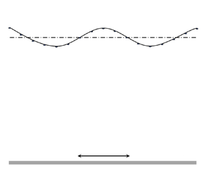
We consider a two-dimensional incompressible viscoelastic liquid film with insoluble surfactant in the horizontal oscillation plane, as shown in figure 1. The density and limiting kinematic viscosity of the fluid are  $\rho$ and
  $\nu$. The oscillation plane is infinite in the
  $x^*$-direction with velocity
  $U_{0}\cos \omega t^*$, where
  $U_{0}$ and
  $\omega$ are the amplitude and frequency of the oscillation, respectively. The superscript ‘
 $*$’ denotes the dimensional variables. The origin is located at the free surface and the upper surface of the film is described by
  $y^* = \eta ^*(x^*, t^*)$. The non-Newtonian liquid film is covered by a monolayer of insoluble surfactant with concentration
  $\varGamma ^*(x^*, t^*)$. Here, the velocity components in the streamwise and vertical directions are represented by
  $u^*_x = u^*$ and
  $u^*_y = \upsilon ^*$, respectively. When the liquid film is at rest, the thickness of the film is
  $d$, as shown by the dash–dotted line in figure 1.

Figure 1. Schematic geometry of the physical system under consideration. A thin viscoelastic film is confined between its deformable free surface  $\eta ^*(x^*, t^*)$ and a horizontal oscillation plane. The dash–dotted line corresponds to the undeformed surface in the quiescent base state.
The governing equations are given by
 \begin{gather} \partial_{i} u^*_{i} = 0, \end{gather}
 \begin{gather}\rho(\partial_{t^*} u^*_{i}+u^*_{j} \partial_{j} u^*_{i}) = \rho g_{i}+\partial_{j} \tau^*_{ij}, \end{gather}
where  $\tau ^*_{i j}$ is stress tensor and the subscript
  $i, j$ are summed over the
  $x^*$- and
  $y^*$-directions. In this paper, Walter's liquid
  $B''$ is considered as the rheological model, which is a first-order elastic approximation of Newtonian behaviour and possesses a rapidly fading memory. The constitutive equation of liquid
  $B''$ is (Beard & Walters Reference Beard and Walters1964; Andersson & Dahl Reference Andersson and Dahl1999)
 \begin{equation} \tau^*_{i j} ={-}p^*\delta_{i j} + 2\rho\nu e^*_{ij}-2M_0\dfrac{\delta}{\delta t^*}e^*_{ij},\end{equation}
where  $p^*$ is the isotropic pressure,
  $\delta _{i j}$ is the Kronecker symbol,
  $e^*_{ij}=(\partial _{i}u^*_j + \partial _j u^*_i)/2$ is the strain rate tensor,
  $2\rho \nu e^*_{ij}$ is the Newtonian stress while
  $2M_0(\delta /\delta {t^*})e^*_{i j}$ corresponds to elastic stress,
  $M_0$ is the viscoelastic coefficient. The corotational derivative of the strain rate tensor is defined as (Shrestha Reference Shrestha1970; Samanta Reference Samanta2017)
 \begin{equation} \dfrac{\delta}{\delta {t^*}} e^*_{ij}=\partial_{t^*} e^*_{ij}+u^*_k \partial_k e^*_{ij}- \partial_k u^*_j e^*_{ik}-\partial_k u^*_i e^*_{kj}. \end{equation}
The corresponding boundary conditions are:
(i) at the bottom of liquid film
 $y^*=-d$,
(2.4a,b)\begin{equation} u^*=U_0\cos\omega t^*, \quad \upsilon^*=0; \end{equation}
$y^*=-d$,
(2.4a,b)\begin{equation} u^*=U_0\cos\omega t^*, \quad \upsilon^*=0; \end{equation}(ii) the kinematic boundary condition at the free surface,
(2.5)\begin{equation} \partial_{t^*}\eta^* = \upsilon^* - u^* \partial_{x^*}\eta^*; \end{equation}(iii) the normal and tangential stresses at the free surface,
(2.6a)\begin{gather} \tau^*_{i j} n_i n_j = \gamma^* \frac{ \partial_{{x^*}{x^*}} \eta^* } {(1+\partial_{x^*}^{2} \eta^*)^{3/2} }, \end{gather}(2.6b)where\begin{gather}\tau^*_{i j} n_j t_i ={-} \frac{ \partial_{x^*} \gamma^* } {(1+\partial_{x^*}^{2} \eta^*)^{{-}1/2} }, \end{gather}$\gamma ^*$ is the surface tension, ${\boldsymbol {n}}$ is the unit normal vector and ${\boldsymbol {t}}$ is the unit tangent vector.


Note that the tangential stress at the free surface is not equal to zero, which is different from that in the work of Samanta (Reference Samanta2017). Owing to the existence of surfactant, the dynamic condition requires a balance between the hydrodynamic traction, the surface tension and the Marangoni traction. The right-hand term of (2.6b) is the Marangoni stress term. The surface tension will depend on the concentration of the local surfactant. For the two-dimensional stability problem, the surfactant concentration  $\varGamma ^*(x^*, t^*)$ is controlled by the following transport equation (Halpern & Frenkel Reference Halpern and Frenkel2003):
 \begin{equation} \partial_{t^*}(H \varGamma^*)+\partial_{x^*}(H \varGamma^* u^*) = D_{s} \partial_{x^*} (H^{{-}1} \partial_{x^*} \varGamma^* ), \end{equation}
where  $H=\sqrt {1+\eta _{x^*}^{*2}}$. Here
  $D_s$ is the surface molecular diffusivity of the surfactant, which can usually be ignored. Considering that the disturbance at the free surface is infinitesimal, the relation between the surface tension
  $\gamma ^*$ and the surfactant concentration
  $\varGamma ^*(x^*, t^*)$ can be approximated as
 \begin{equation} \gamma^* = \gamma_0 -E( \varGamma^*-\varGamma_{0} ), \end{equation}
where  $E$ is the surface elasticity and is a constant,
  $\varGamma _0$ is the basic value of the surfactant concentration, corresponding to a uniform surface tension
  $\gamma _0$.
To normalize the governing equation and boundary conditions, the following characteristic scales are introduced. The mean thickness of liquid film  $d$ is selected as the characteristic length scale,
  $\nu /d$ as the velocity scale,
  $1/\omega$ as the time scale, and
  $\rho \nu ^2/d^2$ as the pressure scale. The surfactant concentration and surface tension are normalized by
  $\varGamma _{0}$ and
  $\gamma _0$, respectively.
Then, a set of dimensionless parameters are obtained as follows:
 \begin{gather} Re=\frac{U_0d}{\nu}, \quad \chi=\frac{gd^3}{2\nu^2}, \quad Ca=\frac{\rho\nu^2}{\gamma_0d},\quad M=\frac{M_0}{\rho d^2},\quad \beta=\sqrt{\frac{\omega d^2}{2\nu}},\quad M_s=\frac{E\varGamma_0}{\rho U_0^2 d}, \end{gather}
where  $Re$ is the Reynolds number, the Galileo number
  $\chi$ is the ratio of gravity force to viscous force, the Capillary number
  $Ca$ shows the effect of the surface tension, the viscoelastic parameter
  $M$ represents the effect of the viscoelasticity, the Womersley number
  $\beta$ is the ratio of the mean thickness of the film to the thickness of the Stokes layer,
  $M_s$ represents the influence of surface surfactant.
For the basic flow, the surface is flat, i.e.  $y=\eta =0$, and we assume that the surface pressure is zero. The surfactant concentration
  $\varGamma$ and surface tension
  $\gamma$ are normalized to unity. By the method of separation of variables, we obtain the unsteady flow solution on the oscillating plane
 \begin{equation} U(y,t)={\rm Re}\left[\dfrac{Re\cosh[\varOmega(1+\mathrm{i}S)y]\mathrm{e}^{\mathrm{i}t}}{\cosh[\varOmega(1+\mathrm{i}S)]}\right],\quad V(y,t)=0, \end{equation}
with
 \begin{equation} S=(1+4M^2\beta^4)^{1/2}+2M\beta^2, \quad \varOmega=\beta \sqrt{ \frac{ (1+4M^2\beta^4)^{1/2} -2M\beta^2}{1+4M^2\beta^4} }. \end{equation}
Here  ${\rm Re}[\cdot ]$ represents the real part of that complex function. The pressure is induced by gravity
 \begin{equation} P(y)={-}2\chi y,\quad -1\leq y\leq 0. \end{equation}
Note that (2.9a–f) is identical to that of Samanta (Reference Samanta2017), which means the surfactant has no effect on the basic flow. This is to be expected physically, as the curvature of the free surface for the basic flow is zero, the effect of surface tension on the basic flow disappears. Besides, when the viscoelastic parameter  $M=0$, (2.9a–f) will degenerate into that of Or (Reference Or1997).
2.2. Linear stability problem
For the linear stability problem, it is assumed that the disturbances are infinitesimal to the basic state (2.9a–f) and (2.12). The non-dimensional variables are
 \begin{equation} u=U+\tilde{u},\quad \upsilon=\tilde{\upsilon}, \quad p=P+\tilde{p}, \quad \varGamma=1+\tilde{\varGamma}, \quad \gamma=1+\tilde{\gamma}. \end{equation}
Considering that the problem we are dealing with is two-dimensional, the continuity in (2.1a) is automatically satisfied by introducing a stream function  $\tilde {\psi }(x,y)$, such that
 \begin{equation} \tilde{u}=\partial_{y}\tilde{\psi}, \quad \tilde{\upsilon}={-}\partial_{x}\tilde{\psi}. \end{equation}
In the following stability analysis, general infinitesimal disturbances for modal analysis are decomposed into the following form:
 \begin{equation} \tilde{\psi}(x,y,t)={\phi}(y,t)\mathrm{e}^{\mathrm{i}k x}, \quad \tilde{\eta}(x,t)=h(t)\mathrm{e}^{\mathrm{i}k x}, \quad \tilde{\varGamma}=\xi(t)\mathrm{e}^{\mathrm{i}k x}, \end{equation}
where  $k \in \mathbb {R}$ is the wavenumber in the streamwise direction. Note that the pressure
  $\tilde {p}$ can be eliminated by combining the Navier–Stokes equations, and hence it does not appear in the linearized system. The time-dependent perturbation equation governing the stability of viscoelastic liquid film is
 \begin{equation} 2 \beta^{2}(\mathscr{L}+M \mathscr{L}^{2}) \partial_{t} \phi=\mathscr{L}^{2} \phi-\mathrm{i} k[U(\mathscr{L}+M \mathscr{L}^{2})-(\mathscr{D}^{2} U+M \mathscr{D}^{4} U)] \phi, \end{equation}
with differential operators  $\mathscr {D}=\partial _{y}$ and
  $\mathscr {L}=\mathscr {D}^2-k^2$. The boundary conditions on the oscillation wall are given by
 \begin{equation} \phi=\mathscr{D} \phi=0, \quad \text{at } y={-}1. \end{equation}
The linearized kinematic boundary condition and transport equation for surfactant are expressed by
 \begin{gather} 2 \beta^{2} \partial_{t} h={-}\mathrm{i} k \phi-\mathrm{i} k U h, \quad \text{at } y=0, \end{gather}
 \begin{gather}2 \beta^{2} \partial_{t} \xi={-}\mathrm{i} k \partial_y\phi - \mathrm{i} k U \xi, \quad \text{at } y=0. \end{gather}
The linearized conditions for the normal and tangential stresses at  $y=0$ are
 \begin{align} 2 \beta^{2}[\mathscr{D}+M(\mathscr{L}-2 k^{2}) \mathscr{D}] \partial_{t} \phi&={-}\mathrm{i} k[U\{\mathscr{D}+M(\mathscr{L}-2 k^{2}) \mathscr{D}\}.\nonumber\\ &\quad +M(\mathscr{D}^{2} U \mathscr{D}-\mathscr{D}^{3} U)] \phi \nonumber\\ &\quad +(\mathscr{L}-2 k^{2}) \mathscr{D} \phi-2 \mathrm{i} k\left(\chi+\frac{k^{2}}{2 Ca}\right) h, \end{align}
 \begin{align} 2 \beta^{2} M(\mathscr{L}+2 k^{2}) \partial_{t} \phi&=(\mathscr{L}+2 k^{2}) \phi- \mathrm{i}kM [U(\mathscr{L}+2 k^{2})-\mathscr{D}^{2} U] \phi \nonumber\\ &\quad +[\mathscr{D}^{2} U-2 \beta^{2} M \mathscr{D}^{2} \partial_{t} U]h + M_s Re^2 \mathrm{i}k\xi. \end{align}
The time-dependent Orr–Sommerfeld equation (2.16) subject to conditions (2.17)–(2.19) forms a Floquet system. For finite-wavelength instabilities, the Floquet system has to be solved numerically, while the long-wavelength instability can be analytically obtained by a series expansion in  $k$, and we will discuss the long-wavelength solutions below.
3. The long-wavelength expansion
According to the Floquet theorem as proposed by Yih (Reference Yih1968), under the limit of long waves, i.e.  $k \ll 1$, the solution can be expanded as follows:
 \begin{gather} \phi(y,t) = \mathrm{e}^{\mu t} [ \phi_0(y,t) + k\phi_1(y,t) + k^2\phi_2(y,t) + \dots ], \end{gather}
 \begin{gather}h(t) = \mathrm{e}^{\mu t} [ h_0(t) + kh_1(t) + k^2 h_2(t) + \dots ], \end{gather}
 \begin{gather}\xi(t) = \mathrm{e}^{\mu t} [ \xi_0(t) + k\xi_1(t) + k^2 \xi_2(t) + \dots ], \end{gather}
where the eigenfunctions  $\phi _j(y,t)$,
  $h_j(t)$ and
  $\xi _j(t)$ (
 $j = 0, 1, 2,\ldots$) are
  $2{\rm \pi}$-periodic in time, the Floquet exponent
  $\mu = \mu _r + \mathrm {i}\mu _i$ is the complex growth rate of the disturbance, and
  $\mu$ is expanded as a power series in
  $k$:
$k$:
 \begin{equation} \mu = \mu_0+k\mu_1+k^2\mu_2+\dots . \end{equation}
Substituting expansions (3.1) and (3.2) into the Floquet system and collecting like terms with different order, a set of coupled partial/ordinary differential equations for  $\phi _j$,
  $h_j$ and
  $\xi _j$ will be obtained, and the equations can be solved sequentially. The basic flow is unstable if there exists at least one Floquet exponent
  $\mu$, with positive real part, i.e.
  $\mu _r > 0$, corresponding to an exponential growth of the disturbance.
For the first order  $O(1)$, the Floquet system can be simplified as
 \begin{gather} \partial_t h_0 + \mu_0 h_0 = 0, \end{gather}
 \begin{gather}\partial_t \xi_0 + \mu_0 \xi_0 = 0. \end{gather}
Since  $h_0$ must be periodic in
  $t$, we have
  $\mu _0=0$,
  $h_0={\rm const}$. and
  $\xi _0={\rm const}$. Otherwise, according to the theory of ordinary differential equations, it can be shown that
  $\mu _0\neq 0$ results in a damping mode
  $h_0 \propto \mathrm {e}^{-\mu _0 t}$. The leading-order approximation can be obtained, as follows:
 \begin{equation} 2\beta^2(\mathscr{D}^2+M\mathscr{D}^4) \partial_t\phi_0 = \mathscr{D}^4\phi_0, \end{equation}
with boundary conditions
 \begin{gather} \phi_0 = \mathscr{D}\phi_0 = 0 \quad \text{at } y={-}1 , \end{gather}
 \begin{gather}2\beta^2 M \mathscr{D}^2 \partial_t \phi_0 = \mathscr{D}^2 \phi_0 + ( \mathscr{D}^2U - 2\beta^2 M \mathscr{D}^2 \partial_t U)h_0 \quad \text{at } y=0, \end{gather}
 \begin{gather}2\beta^2( \mathscr{D} + M \mathscr{D}^3 ) \partial_t \phi_0 = \mathscr{D}^3 \phi_0 \quad \text{at } y=0. \end{gather}
Solving (3.4) and (3.5), the first-order solution for  $\phi _0(y,t)$ can be expressed as
 \begin{equation} \phi_0(y,t)= \mathrm{Re}\left[\dfrac{Re\{1-\cosh[\varOmega(1+\text{i}S)(y+1)]\}{\rm e}^{\text{i}t}}{\cosh^2 [\varOmega(1+\text{i}S)]}\right]h_0. \end{equation}
Note that the Marangoni number does appear in (3.4) and (3.5), so the basic flow at leading-order is not affected by surfactant.
For  $O(k)$, the kinematic condition and the transport equation are
 \begin{gather} 2\beta^2(\mu_1 h_0 + \partial_t h_1) ={-}\text{i}[\phi_0+U h_0], \end{gather}
 \begin{gather}2\beta^2(\mu_1 \xi_0 + \partial_t \xi_1) ={-}\text{i}[U \xi_0+\mathscr{D} \phi_0], \end{gather}
where  $\phi _0$ and
  $U(0,t)$ are periodic in
  $t$. It is necessary to set
  $\mu _1=0$ to ensure that
  $h_1(t)$ and
  $\xi _1(t)$ have periodic solutions. Then, the expressions of
  $h_1(t)$ and
  $\xi _1(t)$ can be obtained, as follows:
 \begin{align} h_1(t)&={-}\dfrac{\mathrm{i}Re}{2\beta^2} \,h_0\,\mathrm{Im}\left[\dfrac{\mathrm{e}^{\mathrm{i}t}}{ \cosh^2[\varOmega(1+\mathrm{i}S)]}\right] +h_1(0), \end{align}
 \begin{align} \xi_1(t)&={-}\dfrac{\mathrm{i}Re}{2\beta^2} \,\xi_0 \,\mathrm{Im}\left[\dfrac{\mathrm{e}^{\mathrm{i}t}}{\cosh[\varOmega(1+\mathrm{i}S)]}\right] \nonumber\\ &\quad+\dfrac{\mathrm{i}Re}{2\beta^2} \,h_0\, \mathrm{Im}\left[\dfrac{[\varOmega(1+\mathrm{i}S)]\sinh[\varOmega(1+\mathrm{i}S)] }{\cosh^2[\varOmega(1+\mathrm{i}S)]}\mathrm{e}^{\mathrm{i}t}\right] + \xi_1(0), \end{align}
where  ${\rm Im}[\cdot ]$ represents the imaginary part of complex function. Here
  $h_1(0)$ and
  $\xi _1(0)$ can set to be zero without loss of generality. Then, the first-order approximation of the Floquet system becomes
 \begin{equation} 2\beta^2(\mathscr{D}^2+M\mathscr{D}^4) \, \partial_t\phi_1 =\mathscr{D}^4\phi_1-\mathrm{i} \, [U(\mathscr{D}^2+M\mathscr{D}^4) -(\mathscr{D}^2U+M\mathscr{D}^4U)] \phi_0, \end{equation}
with boundary conditions
 \begin{equation} \phi_1 = \mathscr{D}\phi_1 = 0 \quad \text{at } y={-}1 , \end{equation}
 \begin{align} 2\beta^2 M \mathscr{D}^2 \partial_t \phi_1 &= \mathscr{D}^2 \phi_1 + [ \mathscr{D}^2 U - 2\beta^2 M \mathscr{D}^2 \partial_t U) \,h_1 \nonumber\\ &\quad -\mathrm{i}M[U\mathscr{D}^2 \phi_0 -\mathscr{D}^2U]\, \phi_0 + \mathrm{i}\xi_0 M_s Re^2 \quad \text{at } y=0, \end{align}
 \begin{align} 2\beta^2(\mathscr{D}+M\mathscr{D}^3) \partial_t\phi_1 &= \mathscr D^3\phi_1-2 \mathrm i \chi h_0 -\mathrm i \, [U(\mathscr D+M\mathscr{D}^3) \nonumber\\ &\quad +M(\mathscr D^2U\mathscr{D}-\mathscr D^3U)]\,\phi_0,\quad\text{at } y=0. \end{align}
Obviously, the right-hand side of (3.10) contains inhomogeneous terms. Both  $U(y, t)$ and
  $\phi _0(y,t)$ are functions with a period of
  $2{\rm \pi}$, so the combination of non-homogeneous term
  $U(y, t)\phi _0(y,t)$ will only lead to a steady part and a function with a period of
  ${\rm \pi}$. In addition, the spatial derivative of
  $\phi _1$ is up to the fourth order, and the solution of the steady part only needs to be assumed to be a cubic polynomial. It can be assumed that
  $\phi _1(y,t) = \phi _1^s(y) + \hat {\phi }_1(y)\mathrm {e}^{\mathrm {i}2t} + \check {\phi }_1(y)\mathrm {e}^{\mathrm {-i}2t}$. Here
  $\phi _1^s(y)$ is the steady part of solution. Similar to the process of Gao & Lu (Reference Gao and Lu2006), it is sufficient to determine the value of
  $\mu _2$ by solving
  $\phi _1^s(y)$. Here, the time-independent solution of first-order equations can be expressed as
 \begin{equation} \phi_1^S(y)=a_1+b_1y+c_1y^2+d_1y^3-2\mathrm{i}Re^2 h_0 \mathrm{Re}[L_0]+2\mathrm{i}Re^2 h_0 \mathrm{Re}[L_1], \end{equation}
with
 \begin{gather} a_1={-}2d_1+\dfrac{\mathrm{i}Re^2A^2(1+\gamma^2)}{\beta^2}(R_2-R_1)h_0 - \frac{\mathrm{i}}{2}\, M_s Re^2\xi_0, \end{gather}
 \begin{gather}b_ 1={-}3d_1+\dfrac{\mathrm{i}\textit{Re}^2A^2(1+\gamma^2)}{\beta^2}R_2 h_0 - \mathrm{i}\, M_s Re^2\xi_0, \end{gather}
 \begin{gather}c_1={-} \frac{\mathrm{i}}{2}\, M_s Re^2\xi_0, \quad d_1= \frac{\mathrm{i}}{3}\,\chi h_0, \end{gather}
 \begin{gather}L_0=\dfrac{\mathrm{i}A^2(1+\gamma^2)(1-4M^2\beta^4)}{8\beta^2S^2}\operatorname{tanh} [\varOmega(1+\mathrm{i}S)]\{S^4\sinh(2\varOmega y)+\mathrm{i}\sin(2\varOmega S y)\}, \end{gather}
 \begin{gather}L_1=\dfrac{\mathrm{i}A^2(1+\gamma^2)}{2\beta^2}\dfrac{\cosh[\varOmega(1+\mathrm{i}S)y]}{ \cosh[\varOmega(1-\mathrm{i}S)]}, \end{gather}
where the expressions of  $A$,
$A$,  $\gamma$,
  $R_1$,
  $R_2$ are the same as those in Samanta (Reference Samanta2017).
For  $O(k^2)$, the Floquet system can be written as
 \begin{gather} 2\beta^2(\mu_2 h_0 + \partial_t h_2) ={-}\text{i}[\phi_1+U h_1], \end{gather}
 \begin{gather}2\beta^2(\mu_2 \xi_0 + \partial_t \xi_2) ={-}\text{i}[U \xi_1+\mathscr{D} \phi_1]. \end{gather}
By taking the steady terms on both sides, (3.20) can be expressed as
 \begin{gather} 2\beta^2\mu_2 h_0 = \left[\frac{A^{2}Re^{2}(1+\gamma^{2})}{\beta^{2}}(R_{2}-R_{1})-\frac{2\chi}{3} \right] h_0 - \frac{Re^2 M_s}{2} \xi_0, \end{gather}
 \begin{gather}2\beta^2\mu_2 \xi_0 = \left[ \frac{A^{2}Re^{2}(1+\gamma^{2})}{\beta^{2}}R_{2}+Re^2 R_3 -\chi\right]h_0 - Re^2 M_s\xi_0, \end{gather}
where  $R_3$ is of the form
 \begin{align} R_3&=\varOmega\{ \sinh(2\varOmega)(1+2S^2) + \sin(2\varOmega S)(S^3+2S) -4M^2\beta^4\sinh(2\varOmega) \nonumber\\ &\quad -4M^2 S^3\beta^4 \sin(2\varOmega S) \}/4S\beta^2 [\cosh(2\varOmega) + \cos(2\varOmega S)]^2. \end{align}
We use the following notation for brevity:
 \begin{gather} I_1 = \frac{A^{2}\textit{Re}^{2}(1+\gamma^{2})}{\beta^{2}}(R_{2}-R_{1}), \end{gather}
 \begin{gather}I_2 = \frac{A^{2}\textit{Re}^{2}(1+\gamma^{2})}{\beta^{2}}R_{2}+\textit{Re}^2 R_3. \end{gather}
Then, (3.21) can be rewritten in the matrix form
 \begin{equation} \begin{bmatrix} \displaystyle{ I_1-\frac{2\chi}{3}} & \displaystyle{ -\frac{\textit{Re}^2 M_s}{2} }\\ \displaystyle{ I_2 -\chi} & \displaystyle{ -\textit{Re}^2M_s}\end{bmatrix} \begin{bmatrix}\displaystyle{ h_0}\\ \displaystyle{\xi_0}\end{bmatrix}= 2\beta^2 \mu_2\begin{bmatrix}h_0\\ \xi_0 \end{bmatrix}. \end{equation}
It should be noted that different from the single formula derived by Samanta (Reference Samanta2017) when solving the Floquet exponent, the transport equation for surfactant is considered here, so the problem needs to deal with the eigenvalue problem of a second-order matrix. In (3.24), the effects of viscoelasticity  $M$ and oscillation frequency
  $\beta$ are included in
  $I_1$ and
  $I_2$. Here
  $2\chi /3$ and
  $\chi$ are the gravity terms. Equation (3.24) constitutes an eigenvalue problem, which determines a set of eigenvalues of
  $\mu _2$ for given different parameters, as well as the corresponding eigenfunctions of
  $h_0$ and
  $\xi _0$. It is not difficult to obtain the analytic solution of its eigenvalue by theoretical derivation. By solving the quadratic equation, we have
 \begin{equation} \theta^{2}+b\theta+c=0, \end{equation}
where  $\theta = 2\beta ^2 \mu _2$,
  $b$ and
  $c$ are the coefficients
 \begin{equation} b=\frac{2}{3}\chi+\textit{Re}^2 M_s-I_1,\quad c=\textit{Re}^2 M_s\left(\frac{I_2}{2}-I_1+\frac{\chi}{6}\right). \end{equation}
If the influence of surfactant is not considered, i.e.  $M_s = 0$, the coefficient
  $b$ will correspond to the terms
  $VECT+GT+ST$ in Samanta (Reference Samanta2017). When the viscoelasticity is absent, (3.24) is the same with Gao & Lu (Reference Gao and Lu2006). And if the viscoelastic and surfactant effects are removed simultaneously, the eigenvalue problem will degenerate into the form of Yih (Reference Yih1968) by reformulating some parameters.
Considering that the coefficients  $b$ and
  $c$ are real, the solution of (3.25) can be two real or conjugate complex roots. According to the analysis of Gao & Lu (Reference Gao and Lu2006), the neutral condition is obtained as
 \begin{equation} \chi=\tfrac{3}{2}\max( 4I_1 - 2I_2, I_1 - \textit{Re}^2 M_s ). \end{equation}
With different parameters, one can determine whether the flow is stable or not by (3.27). In the following analysis, we will discuss the influence of surfactants on the stability of viscoelastic liquid films in the absence and presence of gravity, respectively.
3.1. Absence of gravity $\chi =0$

In some microgravity environments, the absence of gravity often occurs, so it is necessary to consider the stability of oscillating liquid film flow in this situation. We can discuss the influence of viscoelastic  $M$ and surfactant
  $M_s$ on neutral stability conditions by directly analysing (3.27). For the long-wavelength instability (
 $k\rightarrow 0$), the neutral condition becomes
 \begin{equation} \max( 4I_1 - 2I_2, I_1 - \textit{Re}^2 M_s ) = 0. \end{equation}
It is worth noting that the expression of (3.28) used here is consistent with Gao & Lu (Reference Gao and Lu2006) in form, but the influence of viscoelasticity is introduced into the expressions  $I_1$ and
  $I_2$ in this paper. Figure 2 displays the influence of viscoelasticity on the
  $(M_s-\beta )$ neutral curve under given partial parameters. For Newtonian fluid (
 $M = 0$), the characteristics of the neutral curves (black solid lines) are consistent with those found by Gao & Lu (Reference Gao and Lu2006), i.e. for a given
  $M_s$, with the increase of
  $\beta$, the flow will alternately show stable and unstable properties in the corresponding frequency interval. And the neutral curve will become a vertical straight line (curve to straight line) with the increase of
  $M_s$, accompanied by the narrowing of the unstable interval. The curve part is mainly controlled by
  $I_1-\textit {Re}^2M_s$ corresponding to the conjugate complex roots (travelling waves), while the vertical straight lines are controlled by
  $2I_1-I_2$ corresponding to the standing waves. For different viscoelastic parameters, there is no qualitative change in these stability characteristics. Nevertheless, with the increase of viscoelasticity, for low frequency oscillation (
 $\beta <6$), the unstable region will be narrowed and move towards the direction of smaller
  $\beta$. In addition, increasing viscoelasticity will also cause the shrinkage position to be raised. For the higher frequency oscillation (
 $\beta >6$), there is no obvious characteristic of the change of the unstable interval in the presence of viscoelasticity.

Figure 2. The neutral curves in the  $M_s\unicode{x2013}\beta$ plane for different viscoelastic parameters when
  $\chi =0, Ca=0.05, \textit {Re}=200$. Here, the black solid, blue dashed and orange dash–dotted lines stand for
  $M = 0$,
  $M = 0.005$ and
  $M = 0.01$, respectively.
In order to explore more clearly the influence of viscoelasticity on different Floquet modes in the presence of surfactants, two groups of typical values of  $M_s$ and
  $M$ are selected. Figure 3 shows the variation of the real part of the growth rate of two Floquet modes with the oscillation frequency
  $\beta$. For comparison, the growth curves of Newtonian fluid (
 $M=0$) and clean surface (
 $M_s=0$) are also shown in black solid lines. According to the result of Gao & Lu (Reference Gao and Lu2006), the existence of surfactants will inhibit the growth of disturbance and make the flow more stable. For a larger
  $M_s$ (see figure 3a), with the increase of viscoelasticity, the growth rate corresponding to the most unstable mode also increases, and the maximum growth rate within the given parameter range does not exceed that of the clean surface. This means that although viscoelasticity promotes the growth of disturbance, the effect of destabilization is not as obvious as the effect of stabilization from surfactant. The increase of viscoelasticity has no obvious effect on the oscillation frequency corresponding to the maximum growth rate (
 $\beta =1.1$), but for high frequency (
 $\beta >4$), the position of the local maximum of the growth rate curve will move in the direction of decreasing frequency (see the inset). Floquet exponents are real numbers in most frequency ranges, which is shown as two branches of the growth rate curve, and the characteristic mode is a standing wave. In a small frequency range, such as
  $1.94<\beta <2.62$ when
  $M=0.01$, the two branches merge into a curve. The Floquet exponent is a pair of conjugate complex numbers, and the positive and negative imaginary parts represent the opposite propagation directions of travelling-wave modes. In figure 3(b), a smaller surfactant parameter (
 $M_s = 10^{-4}$) is introduced, and it is found that when the viscoelasticity is large enough, the flow is still more unstable than that of Newtonian fluid with a clean surface, despite the presence of surfactant. Therefore, when surfactant and viscoelasticity exist at the same time, the stability of oscillating liquid film depends on their competitive relationship.

Figure 3. The real part of  $\theta /\textit {Re}^2$ as functions of
  $\beta$ when
  $\textit {Re}=200$ for (a)
  $M_s=0.01$ and (b)
  $M_s=10^{-4}$ with
  $M=0$ (black dashed lines),
  $M=0.005$ (orange solid lines) and
  $M=0.01$ (blue dash–dotted lines). The black thin lines represent Newtonian fluids without surfactants.
3.2. Presence of gravity $\chi =1$

When the influence of gravity is considered, the neutral curves corresponding to long-wave instability present the U-shaped curves with separated bandwidth of frequency. Underneath the curve and outside the bandwidth range, all infinitesimal long-wave disturbances are stable. Dandapat & Gupta (Reference Dandapat and Gupta1975) and Samanta (Reference Samanta2017) studied the viscoelastic liquid film on the clean surface, and Gao & Lu (Reference Gao and Lu2006) also studied the Newtonian liquid film containing surfactants. Here, we consider both viscoelastic and surfactant effects. Figure 4(a) shows the influence of different viscoelastic parameters on the neutral curve when  $M_s=0.01$ is fixed. For low-frequency oscillation (
 $\beta < 3$), the neutral curves corresponding to different viscoelastic parameters are all stacked together, which means that viscoelasticity hardly affects the stability of low-frequency oscillation liquid film. When
  $4<\beta <6$, with the increase of viscoelasticity, the critical Reynolds number and the imposed oscillation frequency gradually decrease. The interesting result is that, high frequency oscillation (
 $\beta >10$) significantly enhances the instability of viscoelastic liquid film, which is different from low-frequency oscillation. The effects of different surfactants on the stability of viscoelastic liquid film are shown in figure 4(b). The neutral curves are plotted in the
  $\textit {Re}\unicode{x2013}\beta$ plane parameterized by the value of
  $M_s$ with fixed
  $M=0.01$. The results show that with the increase of
  $M_s$, the unstable frequency bandwidth decreases gradually and the corresponding Reynolds number increases. Similar to the results in the absence of gravity, the surfactant will still weaken the instability of viscoelastic liquid film and make the flow more stable in the presence of gravity. It is worth mentioning that the scattered points (
 $M_s = 0.01$) and thin lines (
 $M_s = 0.001$) of the second and third family neutral curves (
 $4<\beta <8$) in figure 4(b) are coincident. This is because with the increase of
  $M_s$, the dominant term of (3.27) changes from
  $I_1-\textit {Re}^2M_s$ to
  $2I_1-I_2$, and
  $M_s$ no longer influences the neutral curve.

Figure 4. The neutral curves in the  $\textit {Re}\unicode{x2013}\beta$ plane for different viscoelastic parameters and surfactants with
  $\chi =1$. (a) Specified surfactant
  $M_s=0.01$, the blue solid lines, black dashed lines and orange solid lines represent
  $M=0$,
  $M=0.005$ and
  $M=0.01$, respectively. (b) Specified viscoelastic parameter
  $M=0.01$, the blue solid lines, black dashed lines, orange solid lines and open circles represent
  $M_s=0$,
  $M_s=10^{-4}$,
  $M_s=10^{-3}$ and
  $M_s=10^{-2}$, respectively.
4. Numerical procedure
In this section, we briefly discuss the numerical method implemented to solve the time-dependent perturbation equations (2.16)–(2.19) for disturbances of arbitrary wavenumbers. According to the Floquet theory, the disturbances can be expanded in the following forms of truncated complex Fourier series:
 \begin{equation} \phi(y,t)=\mathrm{e}^{\mu t}\sum_{n={-}K}^K \hat{\phi}_n(y) \mathrm{e}^{ \mathrm{i}nt }, \quad h(t)=\mathrm{e}^{\mu t} \sum_{n={-}K}^K \hat{h}_n \mathrm{e}^{ \mathrm{i}nt }, \quad \xi(t)=\mathrm{e}^{\mu t} \sum_{n={-}K}^K \hat{\xi}_n \mathrm{e}^{ \mathrm{i}nt }. \end{equation}
By substituting (4.1a–c) into perturbation equations (2.16)–(2.19) and collecting the coefficients of Fourier components  $\mathrm {e}^{\mathrm {i}nt}$, the matrix differential equations are obtained as
 \begin{equation} \boldsymbol{\mathsf{A}} \hat{\phi}_{n-1} + \boldsymbol{\mathsf{B}}(n) \hat{\phi}_n + \boldsymbol{\mathsf{C}} \hat{\phi}_{n+1} = \mu\boldsymbol{\mathsf{S}}_1 \hat{\phi}_n, \end{equation}
with
 \begin{gather} \boldsymbol{\mathsf{A}} = \mathrm{i}k[(\mathscr{D}^2 U_+ + M\mathscr{D}^4 U_+ )-U_+(\mathscr{L}+M\mathscr{L}^2)], \end{gather}
 \begin{gather}\boldsymbol{\mathsf{B}}(n) = [\mathscr{L}^2 - 2\mathrm{i}n\beta^2 (\mathscr{L}+M\mathscr{L}^2), \end{gather}
 \begin{gather}\boldsymbol{\mathsf{C}} = \mathrm{i}k[(\mathscr{D}^2 U_- + M\mathscr{D}^4 U_- )-U_-(\mathscr{L}+M\mathscr{L}^2)], \end{gather}
 \begin{gather}\boldsymbol{\mathsf{S}}_1 = 2 \beta^2 (\mathscr{L} +M \mathscr{L}^2), \end{gather}
where  $U_+$ and
  $U_-$ are defined as
  $U(y,t)=U_+(y)\mathrm {e}^{\mathrm {i}t}+U_-(y)\mathrm {e}^{\mathrm {-i}t}$. The linearized kinematic boundary condition and transport equation (2.18) are
 \begin{gather} {\mathrm{i} k U_+ } \hat{h}_{n-1} + 2\mathrm{i}\beta^2 n\hat{h}_{n} + \mathrm{i}kU_- \hat{h}_{n+1} + \mathrm{i}k \hat{\phi}_{n} ={-}2 \mu \beta^2\hat{h}_n, \end{gather}
 \begin{gather}{\mathrm{i} k U_+ } \hat{ \xi }_{n-1} + 2\mathrm{i}\beta^2 n\hat{\xi}_{n} + \mathrm{i}kU_-\hat{\xi}_{n+1} + \mathrm{i}k \mathscr{D} \hat{\phi}_{n} ={-}2 \mu \beta^2\hat{\xi}_n. \end{gather}
 The system of equations (4.2)–(4.4) is solved numerically using the Chebyshev spectral collocation method (Schmid & Henningson Reference Schmid and Henningson2001). Considering that the Chebyshev polynomials are defined over the domain  $[-1, +1]$, we need to map the computational domain onto the physical domain
  $[-1,0]$. Then, the continuous function is discretized on the Gauss–Lobatto collocation points and the differential operators are replaced by pseudospectral matrix approximations. Each function of
  $\hat {\phi }_{n}(y)$ is represented as a vector of its function values on Gauss–Lobatto points. The linear system (4.2)–(4.4) can be turned into a matrix eigenvalue problem
 \begin{equation} \boldsymbol{\mathsf{R}}\boldsymbol{\mathsf{X}} =\mu \boldsymbol{\mathsf{S}}\boldsymbol{\mathsf{X}}, \end{equation}
where  $\boldsymbol{\mathsf{R}}$ is a block tridiagonal matrix, which is composed of matrices
  $\boldsymbol{\mathsf{A}}$,
  $\boldsymbol{\mathsf{B}}(n)$ and
  $\boldsymbol{\mathsf{C}}$, and
  $\boldsymbol{\mathsf{S}}$ is a block diagonal square matrix. Here
  $\boldsymbol{\mathsf{X}} = [\hat {\phi }_{-K} \cdots \hat {\phi }_{K} \ \hat {h}_{-K} \cdots \hat {h}_{K} \hat {\xi }_{-K}\cdots \hat {\xi }_{K}]^{\rm T}$ is a column matrix. The boundary conditions are treated carefully by replacing the rows in the corresponding positions in the matrices
  $\boldsymbol{\mathsf{R}}$ and
  $\boldsymbol{\mathsf{S}}$. Finally, the eigenvalues
  $\mu$ and eigenvectors
  $\boldsymbol{\mathsf{X}}$ are obtained by solving the generalized eigenvalue problem of sparse matrix
  $\boldsymbol{\mathsf{R}}$ and
  $\boldsymbol{\mathsf{S}}$. The purpose of numerical simulation is to find the neutral stability curve, i.e. for given parameters, the real parts of Floquet exponent
  $\mu$ is zero. For the eigenvalues with negative real parts, (
 $\mu _r < 0$) will provide stable modes and are not relevant for the instability analysis.
For different parameters (e.g. capillary number,  $Ca$; Womersley number,
  $\beta$; and viscoelastic parameter,
  $M$), several tests have been performed for different Chebyshev points
  $N$ and Fourier modes
  $K$ to ensure numerical convergence. Table 1 shows the results of numerical convergence tests for typical parameters. In the calculation, the number of
  $N$ and
  $K$ is increased until the Floquet exponents
  $\mu$ obtained are accurate enough. The long-wavelength analytical results of (3.27) are also shown in table 1 (marked in bold) to validate the numerical method. Further increasing the values of
  $N$ and
  $K$ by five, the relative error of eigenvalues varies by less than
  $10^{-10}$, but it will consume more computational resources. Thus, in most subsequent numerical calculations, the number of Chebyshev points
  $N=24$ and Fourier modes
  $K=12$ are used to accurately compute the eigenvalue problem. For
  $\beta >8$ with large value of wavenumber,
  $N=40$ and
  $K=20$ are also used to check the accuracy of the calculations.
Table 1. Numerical results of convergence tests for Chebyshev points  $N$ and Fourier modes
  $K$ when
  $\textit {Re}=100$,
  $\beta =6$,
  $\chi =1$,
  $Ca=0.05$ and
  $M_s=0.001$. The values marked in bold indicate the long-wavelength expansion results of (3.27).

When viscoelasticity is not considered ( $M=0$), we compare the numerical results with those of Gao & Lu (Reference Gao and Lu2008). In the absence of gravity, the results for fixed values of
  $\textit {Re}=0.5$,
  $\beta =3$,
  $Ca=0.05$ and
  $M_s=0.001$ are shown in table 2. The first four eigenvalues obtained under these parameters are
  $\mu _1 \sim \mu _4$. Here
  $\mu _1$ corresponds to the trivial solution and is not shown. Here
  $\mu _2$ and
  $\mu _3$ are complex conjugates and
  $\mu _4$ is real. It is observed that the current results agree well with the results from Gao & Lu (Reference Gao and Lu2008).
Table 2. Comparison of theoretical (T) and numerical (N) results for  $\mu _2, \mu _3$ and
  $\mu _4$ with
  $\textit {Re}=0.5$,
  $\beta =3$,
  $\chi =0$,
  $Ca=0.05$,
  $M=0$ and
  $M_s=0.001$.

In order to further verify the accuracy of the current code and the correctness of the long-wavelength analysis results, we compare the analytical solution of the long-wavelength limit obtained in § 3 with the current numerical results. Actually, these two results can be verified by each other. The eigenvalue given by (3.24) for  $k \ll 1$ can be approximated as
  $\mu = k^2 \theta /(2\beta ^2)$. Figure 5 illustrates the comparison between the approximate analytical solution and the numerical solution in the range of
  $10^{-4}$–
 $10^{-1}$, and the typical parameters
  $\chi =1,$
  $Ca=0.05,$
  $M=0.01,$
  $M_s=10^{-2}$ and
  $\textit {Re}=200$ are selected. The Floquet exponent is conjugate complex when
  $\beta =2$ as shown in figure 5(a). The real part of
  $\mu$ is positive at different
  $k$, which means the disturbance increases under this parameter, which eventually leads to instability of the flow. It is reasonable to note that the numerical results gradually deviate from the long-wavelength theoretical solution when
  $k > 0.01$, because the theoretical results will gradually become invalid with the increase of
  $k$. However, for
  $k < 0.01$, the numerical results are in good agreement with the theoretical solutions. Figure 5(b) shows the absolute values of the first and second eigenvalues
  $\mu _1$ and
  $\mu _2$ of the most ‘dangerous’ mode for
  $\beta =3$. Since
  $\mu _1$ and
  $\mu _2$ are real, their corresponding modes are standing waves. Similarly, the numerical results are consistent with theoretical solutions for small values of
  $k$. After verifying the numerical convergence and the correctness of the results at different wavelengths (long- and finite-wavelength), we concluded that the results of numerical procedure are reassuringly in very good agreement with previously available data.

Figure 5. Comparison of long-wave approximation results (solid lines) and numerical results (scatters) for  $\chi =1,$
  $Ca=0.05,$
  $M=0.01,$
  $M_s=10^{-2}$ and
  $\textit {Re}=200$. (a) Complex conjugate
  $\mu$ for
  $\beta =2$, the blue and orange solid lines represent the real part
  $\mu _r$ and imaginary part
  $\mu _i$, respectively. (b) The first two real eigenvalues for
  $\beta =3$, the blue and orange solid lines represent the first eigenvalue
  $\mu _1$ and the second eigenvalue
  $\mu _2$, respectively.
5. Finite-wavelength instability
In this section, we will discuss the stability of viscoelastic oscillating liquid film containing surfactants under arbitrary wavelength disturbance. According to the results of long-wavelength analysis in § 3, the presence of surfactant on the surface of the liquid film plays a vital role in stability. Both clean surface ( $M_s=0$) and the existence of surfactant will be considered with or without gravity in this section. For comparison, we choose the same parameters as those in Or (Reference Or1997) and Gao & Lu (Reference Gao and Lu2008), i.e.
  $Ca = 0.05$,
  $\chi = 0$ or 1, and the stability characteristics will be analysed by varying
  $\beta$,
  $\textit {Re}$,
  $M_s$ and
  $M$.
$M$.
5.1. Clean surface in the absence/presence of gravity
The influences of viscoelasticity in the presence of gravity are considered by Samanta (Reference Samanta2017). However, the results of the absence of gravity are not involved in his work. Before considering the combined effects of viscoelasticity and surfactant, let us briefly analyse the stability of clean-surface viscoelasticity liquid film without gravity. Figure 6 shows the Reynolds number and its corresponding wavenumber versus imposed frequency for two viscoelastic parameters ( $M=0.005$ and 0.01). As described in the results of long-wavelength stability, the disturbances are unstable over alternating frequency intervals, and the boundaries of unstable regions are indicated by vertical dash–dotted lines in figures 6(a) and 6(c). Different from the long-wavelength results, when the Reynolds number exceeds the critical value, finite-wavelength instability occurs in the region where the long-wavelength disturbance is stable. If
  $\beta$ continues to increase to the next long-wavelength instability interval, although the finite-wavelength instability still exists (see the blue dotted lines), the critical Reynolds number
  $\textit {Re}_c$ is not determined by the finite-wavelength disturbance due to the long-wave mode being still unstable when
  $\textit {Re}\rightarrow 0$. These phenomena are similar to those found by Gao & Lu (Reference Gao and Lu2008). In addition, the neutral curve in the presence of gravity (
 $\chi = 1$) is also given in figure 6(a), in which the U-shaped curve represents the result of the long-wavelength instability. It can be seen that with the increase of
  $\beta$, the flow instability is first dominated by the long-wave mode. When
  $\beta$ increases to 2.4925, the critical Reynolds number corresponding to the long-wave mode is equal to that of the finite-wavelength, and then the oscillation frequency range is dominated by the finite-wavelength mode until the neutral curve intersects the second U-shaped neutral curve. Thus, in the presence of gravity,
  $\textit {Re}_c$ is a continuous function of the imposed frequency, although the long-wavelength mode and the finite-wavelength mode alternate with increasing frequency, which is quite different from the results in the absence of gravity. Two points should be noted in figures 6(a) and 6(c). On the one hand, the critical Reynolds number corresponding to a finite-wavelength seems to be insensitive to gravity except for near
  $\beta =8$, which can be seen from the coincidence of the neutral curves
  $\chi = 0$ (blue solid lines) and
  $\chi = 1$ (open circles). In fact, for
  $\beta =3$ in figure 6(a), the critical Reynolds number corresponding to
  $\chi = 1$ is 58.95, while that corresponding to
  $\chi = 0$ is 59.77, with a difference of only
  $1.37\,\%$. On the other hand, the oscillation frequencies corresponding to the bifurcation points in the presence of gravity (orange solid circle) and the absence of gravity (open diamond) are also affected slightly by gravity. For example,
  $\beta$ values corresponding to the presence and absence of gravity at the first bifurcation point are 2.4925 and 2.5564, respectively. Considering that gravity has little influence on the boundary of the stability region and the critical Reynolds number, the results with or without gravity will not be distinguished in the following analysis unless otherwise specified.

Figure 6. Stability characteristics in the absence of surfactants with  $Ca=0.05$ for different viscoelastic parameters
  $M=0.005$ (a,b) and
  $M=0.01$ (c,d). Panels (a,c) represent the stability boundaries in the (
 $\beta, \textit {Re}$)-plane and panels (b,d) represent variation of the corresponding wavenumber
  $k$ with
  $\beta$. The U-shaped orange solid lines and open circles represent long- and finite-wavelength instability for
  $\chi =1$. The blue solid lines represent finite-wavelength instability for
  $\chi =0$. The vertical dash–dotted lines represent the boundaries of unstable regions for
  $\chi =0$.
For the larger viscoelasticity ( $M=0.01$), as shown in figure 6(c),
  $\textit {Re}$ increases with the increase of
  $\beta$ for the low-frequency oscillation (
 $2.4970 < \beta < 3.86$), while in the high-frequency region (
 $8.014 < \beta < 11.22$),
  $\textit {Re}$ shows a decreasing trend, i.e. Reynolds number does not always monotonically increase with the imposed frequency. In addition, when the flow instability changes from long-wavelength mode to finite-wavelength mode, the critical wavenumber does not necessarily change continuously, as shown in figure 6(d). The discontinuity of wavenumber is explained as follows. For
  $\chi =0$, the first branch point (
 $\text {P}_1$) is located at
  $\beta _1=2.4968$, and we plot the neutral curves for the slightly higher and lower values of
  $\beta _1$ in figure 7(a). It can be seen that for
  $\beta =2.4970$ (orange solid line), the critical wavenumber corresponding to the local minimum of the neutral curve is 0.2, while for
  $\beta =2.4967$ (blue solid line), the neutral curve monotonically increases from the coordinate origin
  $(k, Re)=(0, 0)$. Therefore, the critical wavenumber can be continuously transitioned from long-wavelength instability to finite-wavelength instability. For the second branch point (
 $\text {P}_2$),
  $\beta _2=5.1305$, the neutral curve for slightly higher frequency has a local minimum at
  $k=0.54$ (see figure 7b), which makes the critical wavenumber discontinuity near
  $\beta _2$. The characteristics of the first two bifurcation points are qualitatively consistent with the results obtained by Gao & Lu (Reference Gao and Lu2008) in the study of oscillating Newtonian fluid films with surfactants. The neutral curve near that third branch point (
 $\text {P}_3, \beta _3=7.9909$) is different from the first two branch points. It first separates a new branch at
  $\text {P}_3$ with a rapid increase in Reynolds number (see blue solid line in figure 6c). Then, in a small range of
  $\beta$, it intersects with another monotonically decreasing neutral curve at
  $\text {P}_4$. It can be seen from figure 6(d), in the
  $k\unicode{x2013}\beta$ plane, the critical wavenumber increases rapidly from zero at first, after that, it appears discontinuous with the increase of
  $\beta$, and continuously changes at a higher wavenumber. Note that the parameters used here are consistent with figure 5 in Samanta (Reference Samanta2017). However, there is no stable bandwidth in the present work for both
  $\chi =0$ and
  $\chi =1$. On the contrary, a neutral curve with finite-wavelength is found. In order to more comprehensively analyse the different structural characteristics of critical parameter changes near
  $\beta _3$, the neutral curves corresponding to different
  $\beta$ on the
  $\textit {Re}\unicode{x2013}k$ plane are plotted in figure 7(c). It can be seen that when the frequency is less than
  $\beta _3$, the neutral curve increases monotonically over the range of
  $0 < k < 0.5$, which may explain why the critical wavenumbers increase from zero. Nevertheless, when the long-wavelength instability is eliminated, the neutral curves corresponding to
  $\beta = 7.991$ contain two local minima which correspond to a small wavenumber of 0.08 and a larger wavenumber of 4.2, respectively. With the increase of
  $\beta$, the Reynolds number corresponding to the extreme point of the smaller wavenumber increases rapidly while that of the larger wavenumber decreases slowly. Until
  $\beta$ increases to 8.014, the two local lowest points have the same Reynolds number
  $\textit {Re}=138.6$ corresponding to the point
  $\text {P}_4$, and then the global minimum of the neutral curve is controlled by the part of large wavenumber. This is why the critical Reynolds number is continuous in figure 6(c) and the corresponding wavenumber jumps from 0.32 to 4.2. It should be noted that the Floquet exponents corresponding to the above critical parameters are all zero, i.e. the characteristic mode always exists as a standing wave.

Figure 7. The neutral curves in the neighbourhood of branch point when  $M=0.01$,
  $M_s=0$,
  $Ca=0.05$ and
  $\chi =0$: (a) first branch point
  $\text {P}_1$; (b) second branch point
  $\text {P}_2$; (c) third branch point
  $\text {P}_3$.
5.2. Effect of surfactants in the absence/presence of gravity
In this section, we will focus on the combined effect of viscoelasticity and surfactants on the stability of oscillating liquid films. The typical parameter  $M_s=0.001$ is selected for analysis. Similar to the previous discussion, the presence or absence of gravity has an extremely limited effect on finite-wavelength stability, as shown in figure 8. Due to the effect of the surfactant on the long-wavelength instability, the bandwidth of each instability interval is shorter than that in the absence of the surfactant, which means that the oscillation frequency range occupied by the finite-wavelength instability will be wider, which can be observed by comparing figure 6(a) with figure 8(a). There are three significant differences in the neutral curve for finite-wavelength instability when considering surfactants. First, in the low-frequency region, with the increase of
  $\beta$, the unstable mode changes from the long-wavelength mode to the finite-wavelength mode. Careful examination of the Floquet exponent reveals that
  $\mu$ corresponding to the finite-wavelength mode is a pair of conjugate complex numbers, which means that the disturbance is a travelling wave. Continue increasing
  $\beta$ to 3.5, where there is a bifurcation point (P) to the right of which corresponds to the higher wavenumber, as shown in figure 8(b). Different from the travelling-wave mode on the left-hand side of the bifurcation point, the mode corresponding to the high wavenumber is a standing-wave. Second, in the intermediate frequency region (
 $4.8<\beta <6.9$), the finite-wavelength neutral curve shows a discontinuity at
  $\beta =6.7$, which is caused by the standing-wave mode competition between two different wavelengths. This case has been analysed in detail in the work of Or (Reference Or1997) and Gao & Lu (Reference Gao and Lu2008), and will not be described here. Third, for the high-frequency region (
 $\beta >7.44$) in figure 8(a), compared with the Newtonian fluid, the critical Reynolds number in the presence of viscoelasticity is no longer monotonically increasing, while the critical wavenumber corresponding to the finite-wavelength mode is gradually increasing with
  $\beta$. More importantly, as shown in figure 8(c), for higher viscoelastic parameters (
 $M=0.01$), the viscoelasticity causes the instability of the oscillating liquid film to be determined by the standing-wave mode of finite wavelength over a relatively large frequency range (
 $4.6<\beta <11.4$). The above results again imply that viscoelasticity has a significant effect on the stability of the high-frequency oscillation liquid film.

Figure 8. Stability characteristics in the presence of surfactants with  $M_s=0.001$ and
  $Ca=0.05$ for different viscoelastic parameters
  $M=0.005$ (a,b) and
  $M=0.01$ (c,d). Panels (a,c) represent the stability boundaries in the (
 $\beta, \textit {Re}$)-plane and panels (b,d) represent variation of the corresponding wavenumber
  $k$ with
  $\beta$. The meanings of curves and symbols are consistent with figure 6.
In order to study the stability characteristics of surfactants to viscoelastic liquid film under finite-wavelength disturbance more clearly, we calculated the variation of critical Reynolds number and critical wavenumber with oscillation frequency for more values of  $M_s$, as shown in figure 9. The left and right endpoints of each curve represent the boundary between long-wave instability and finite-wavelength instability. Figures 9(a) and 9(b) show the effects of surfactants on the critical Reynolds number and critical wavenumber in the low-frequency range, respectively. In order to better distinguish the differences between different curves, in figure 9(a), the same method is adopted as in Gao & Lu (Reference Gao and Lu2008) to deal with the ordinate. It can be seen that with the increase of
  $M_s$, the range of finite-wavelength instability widens, which is discussed in the long-wavelength stability analysis considering gravity (see figure 4b). Different surfactant concentrations will lead to the competition between travelling-wave mode and standing-wave mode. For example, when
  $M_s=0$, the unstable mode is a standing wave, but when the surfactant concentration is very small (
 $0 < M_s \leq 10^{-4}$), the unstable mode becomes a travelling wave. And with the increase of
  $M_s$, the critical Reynolds number increases, which means that surfactants can make the flow more stable. Further increasing the influence of surfactant (
 $M_s = 10^{-3}$ or
  $10^{-2}$), the critical curve becomes two branches. The left-hand branch represents the travelling-wave mode with a smaller critical wavenumber, while the right-hand branch represents the standing-wave mode and has a large critical wavenumber. With the increase of
  $M_s$, the intersection of the two branches will move in the direction of decreasing oscillation frequency. Nevertheless, the flow in the presence of surfactant with
  $M_s \leq 10^{-2}$ is always more stable than that in the absence of surfactant. When
  $M_s$ is large enough, e.g.
  $M_s=10^{-1}$, the unstable modes in the whole low-frequency oscillation range are standing waves, which is consistent with the clean-surface case. In addition, the curve of
  $M_s = 0$ and the curve of
  $M_s = 10^{-1}$ intersect, which means that whether the flow is stabilized or destabilized by the surfactant depends on the oscillation frequency of the plate. The effects of surfactants on critical Reynolds number and critical wavenumber in higher frequency range are shown in figures 9(c) and 9(d). For the clean-surface case, the unstable mode is still a standing wave, and the curve is discontinuous in the range of
  $6.76<\beta <7.92$, which is dominated by long-wavelength instability. When the concentration of surfactant is increased,
  $M_s = 10^{-5}$ or
  $10^{-4}$, the unstable mode will change from a travelling wave to a standing wave with the increase of
  $\beta$, and the oscillation frequencies at the mode change points are
  $\beta =8.4$ and 5.4, respectively, which are marked by arrows in figure 9(d). When
  $M_s$ is further increased,
  $M_s=10^{-3}$, the unstable mode reverts to the standing-wave type, and the discontinuity in the unstable curve is caused by the competition of different standing-wave modes. It is worth mentioning that surfactants can promote or inhibit flow stability at both lower and higher oscillation frequencies.

Figure 9. Effects of surfactants on the finite-wavelength instability characteristics of the flow in different frequency range with  $\chi =1$,
  $Ca=0.05$ and
  $M=0.01$. Variation of (a)
  $\text {e}^{-\beta }\textit {Re}$ and (b) the corresponding critical wavenumber
  $k$ with
  $\beta$ in low-frequency. Variation of (c)
  $\textit {Re}$ and (d) the corresponding critical wavenumber
  $k$ with
  $\beta$ in higher frequency.
6. Conclusion
In this work, we have studied the linear instability of viscoelastic film with insoluble surfactants on an oscillating plane for disturbances with arbitrary wavenumbers. Floquet theory is utilized to describe the combined effects of viscoelastic and insoluble surfactants on the linear instability of oscillating liquid film. The time-dependent perturbation equations governing the stability of viscoelastic liquid film are derived for an unsteady basic flow. Then, the solution of the eigenvalue problem is derived analytically by the asymptotic expansion method in the limit of long-wavelength perturbations. The finite-wavelength instability is solved numerically by utilizing the Chebyshev spectral collocation method. The theoretical solution of the long wave and the numerical solution of the finite wavelength are consistent when  $k\ll 1$.
The flow is governed by five parameters: Reynolds number  $\textit {Re}$; viscoelastic parameter
  $M$; surface surfactant
  $M_s$; Galileo number
  $\chi$; Womersley number
  $\beta$. The present parametric study is mainly focused on the critical mode of the linear problem. The main conclusions of the analysis are as follows. For long-wavelength instability, the presence of viscoelasticity shifts the stability boundaries to the low-frequency region for
  $\beta <6$ and
  $\chi =0$. The growth rate corresponding to the most unstable mode increase with the increasing
  $M$. When considering the effect of gravity, the U-shaped neutral curves with separation bandwidth appear. For low-frequency oscillation (
 $\beta < 3$), the viscoelasticity almost has no effect on the stability, while high-frequency oscillation significantly enhances the instability of viscoelastic liquid film. Besides, the presence of surface surfactants will decrease the unstable frequency bandwidth and increase the corresponding Reynolds number. For finite-wavelength instability, we first discuss the stability of the clean surface in the absence/presence of gravity. The critical parameters corresponding to a finite wavelength seem to be insensitive to gravity except for near
  $\beta =8$. Different from the results of Samanta (Reference Samanta2017), four branch points are detected and the neutral curves are plotted near those branch points. Finally, the combined influence of viscoelasticity and surfactants on the stability are also considered. Both travelling-wave mode and standing-wave mode are found due to the existence of surface surfactants. For high-frequency oscillation plane, increasing viscoelastic parameters will cause the critical Reynolds number to increase non-monotonically and the instability to be determined by the finite-wavelength mode over a relatively large frequency range. The above conclusions suggest that viscoelasticity has a great influence on the stability of liquid film with high-frequency oscillation. In addition, for fixed viscoelastic parameter
  $M=0.01$, different surfactant concentrations will lead to the competition between travelling-wave mode and standing-wave mode. When
  $M_s$ is large enough, the disturbance modes in the form of a standing wave dominate the instability of the flow for finite-wavelength disturbance. And the flow can be stabilized or destabilized by the surfactant depending on the oscillation frequency of the plate.
Although only infinitesimal disturbances are considered in this paper, the present configuration can be extended to analyse the finite-amplitude instability. For non-Newtonian flow, only Walter's liquid  $B''$ is considered here and it is also necessary to study the stability of other rheological models. In addition, the experimental or numerical simulation data are needed as a supplement to the theoretical results, which will be the subject of future exploration. Despite this, we anticipate that the results provided in this paper may serve as a guide for the sequence of bifurcation leading to turbulence for such a flow system driven by an oscillating wall.
Acknowledgements
The authors would like to thank the anonymous referees for their suggestions to improve the manuscript.
Funding
This work was supported by the Natural Science Foundation of Shandong Province (nos. ZR2022QA090, ZR2022MA033) and the National Natural Science Foundation of China (no. 12072177).
Declaration of interests
The authors report no conflict of interest.


