


1. Introduction
The chaotic nature of turbulent flows and their importance in physical and engineering systems has motivated countless studies attempting to obtain simplified models for control purposes in engineering applications. In particular, unbounded shear flows such as jets and wakes have received unabated interest due to their importance for drag reduction, control of unsteady loads, mixing enhancement, etc.
Despite their chaotic nature, such flows are characterized by recurrent flow patterns that are typically referred to as coherent structures. The beauty of the coherent structures has fascinated scientists since Leonardo da Vinci (Marusic & Broomhall Reference Marusic and Broomhall2021) and has hinted at the possibility that the flow dynamics can be represented as a system evolving on a low-dimensional attractor. Proper orthogonal decomposition (POD) (Berkooz, Holmes & Lumley Reference Berkooz, Holmes and Lumley1993), also called principal component analysis in statistics, has received significant attention since it allows decomposing a flow field into orthogonal modes sorted according to their contribution to the variance of the quantity to be analysed. One of the most exploited advantages of POD in fluid mechanics is its capability to simplify the Navier–Stokes equations into a system of ordinary quadratic differential equations employing Galerkin projections (Noack et al. Reference Noack, Afanasiev, Morzyński, Tadmor and Thiele2003). Low-order models obtained from POD open a door to a vast space of applications such as flow control (Brunton & Noack Reference Brunton and Noack2015) and also crisp least-order models for bifurcations and interactions of coherent structures (Deng et al. Reference Deng, Noack, Morzyński and Pastur2020).
A myriad of POD studies hint at low-dimensional manifolds describing turbulent shear flows. In the case of oscillatory flows, two-dimensional manifolds have been identified from laminar two-dimensional cylinder flows (Noack et al. Reference Noack, Afanasiev, Morzyński, Tadmor and Thiele2003) to experimental turbulent wakes behind finite cylinders at high Reynolds numbers (Bourgeois, Martinuzzi & Noack Reference Bourgeois, Martinuzzi and Noack2013). These manifolds are the cornerstone of mean-field Galerkin models. Even flows with several frequencies may live on a mean-field manifold (Luchtenburg et al. Reference Luchtenburg, Günter, Noack, King and Tadmor2009). The pioneering POD model of Aubry et al. (Reference Aubry, Holmes, Lumley and Stone1988) derives such a manifold for the turbulent boundary layer from the Reynolds equations. For more complex flows, the energy spectrum of POD typically reveals  $O(10)$ distinct most-energetic eigenvalues associated with physically interpretable modes. This distinct spectrum is usually followed by a steadily decreasing eigenvalue distribution with less interpretable and increasingly fine-scaled modes. More rigorously, if states have finite variance, the covariance operator for POD is positive trace class, hence compact, (see, e.g. theorem 4.1 in the book by Minh & Murino (Reference Minh and Murino2017)) and so its non-zero spectrum consists of isolated eigenvalues that are either a finite set or converge to 0 (see, e.g. theorem 6.8 in the book by Brezis (Reference Brezis2011)). The distinct POD mode amplitudes can be conceptualized as the conductors of a large ‘slaved’ turbulence orchestra (Callaham, Brunton & Loiseau Reference Callaham, Brunton and Loiseau2022).
While the focus of POD is on obtaining reduced-order models optimal in terms of energy, the field of statistical learning provides a vast number of tools for dimensionality reduction (Franklin Reference Franklin2005). Multidimensional scaling (MDS), for instance, is based on the singular value decomposition of the data distance matrix and allows representing a dataset in a low-dimensional space preserving the distance between the snapshots in the high-dimensional space (Torgerson Reference Torgerson1952; Kruskal Reference Kruskal1964). Multidimensional scaling has been used in fluid mechanics mainly for visualization purposes and effectively captures some hidden features of the flows (Kaiser et al. Reference Kaiser, Noack, Cordier, Spohn, Segond, Abel, Daviller, Östh, Krajnović and Niven2014; Foroozan et al. Reference Foroozan, Guerrero, Ianiro and Discetti2021).
The capability of obtaining low-dimensional representations is tempting to identify embedded manifolds of the flows under study. Manifold learning attempts to recognize a low-dimensional surface, the manifold, near which the dataset actually resides. In statistical language, the dataset can be described to lie on or near a manifold in a low-dimensional space in which the manifold expresses some basic features of it. In this sense the manifold is in fact the set of relations that connect snapshots to each other. Interestingly, often high-dimensional systems appear to evolve on low-dimensional manifolds, thus simplifying their modelling if the manifold can be identified. These aspects pushed the development of the manifold learning techniques in the last decades. Remarkable examples are locally linear embedding (Roweis & Saul Reference Roweis and Saul2000), isometric mapping (Tenenbaum, de Silva & Langford Reference Tenenbaum, de Silva and Langford2000) and diffusion maps (Coifman & Lafon Reference Coifman and Lafon2006).
The traditional dimensionality-reduction methods are structured on linear models and thus fail in capturing the manifolds when a nonlinear structure is present in the data. Turbulent flows exhibit a nonlinear behaviour which motivates the investigation of nonlinear models for manifold learning. As reported by Gorban & Karlin (Reference Gorban and Karlin2005), manifold learning falls in the field of model engineering, which attracts a wide interest among physics, mathematics and engineering, as is also evident from the three-volume book on model-order reduction by Benner et al. (Reference Benner, Schilders, Grivet-Talocia, Quarteroni, Rozza and Silveira2020a,Reference Benner, Schilders, Grivet-Talocia, Quarteroni, Rozza and Silveirab, Reference Benner, Grivet-Talocia, Quarteroni, Rozza, Schilders and Silveira2021). For instance, autoencoders are increasingly used in fluid mechanics as a nonlinear dimensionality reduction architecture (Lee & Carlberg Reference Lee and Carlberg2020). The fluid mechanics community has exploited the approximation of the Koopman operator to obtain nonlinear embeddings of fluid flows (Mezic Reference Mezic2013; Otto & Rowley Reference Otto and Rowley2021). Koopman modes are, for nonlinear dynamics, analogous to normal modes in linear problems, provided that the nonlinear dynamics are represented in the infinite-dimensional space of all possible observable measurements of the system. Giannakis et al. (Reference Giannakis, Kolchinskaya, Krasnov and Schumacher2018) reported an insightful application of Koopman eigenfunction analysis on a complex three-dimensional flow such as a turbulent Rayleigh–Bénard convection cell. However, the identification of finite-dimensional coordinate systems in which the dynamics appear approximately linear remains an open challenge (Brunton et al. Reference Brunton, Budisic, Kaiser and Kutz2022). As shown by Morton et al. (Reference Morton, Jameson, Kochenderfer and Witherden2018) low-dimensional nonlinear dynamical models can be able to predict the cylinder wake and eventually be employed for model predictive control (resulting in simple, interpretable control laws).
Tenenbaum et al. (Reference Tenenbaum, de Silva and Langford2000) have shown that the dimensionality reduction based on geodesic distances can be a powerful tool in preserving the actual behaviour of nonlinear datasets. This technique is referred to as isometric feature mapping, or Isomap. Despite the importance of identifying the manifold dimension for the modelling, prediction, control and understanding of fluid flows, surprisingly, the application of Isomap in fluid mechanics is minimal. Tauro, Grimaldi & Porfiri (Reference Tauro, Grimaldi and Porfiri2014) successfully employed Isomap to identify manifolds from flow-visualization data while others used it for combustion (Bansal, Mascarenhas & Chen Reference Bansal, Mascarenhas and Chen2011), and design optimization (Franz et al. Reference Franz, Zimmermann, Görtz and Karcher2014). Recently Otto & Rowley (Reference Otto and Rowley2022) discussed the limitation of the linear methods in the case of selection and placement of sensors in a flow field.
This manuscript introduces a framework of manifold learning as an encoder for unbounded shear flows with a  $K$-nearest neighbours (
 $K$NN) decoder. The input snapshots, which can be obtained either from a simulation or an experiment, are encoded using Isomap as the primary tool. The high-dimensional space transforms to a low-dimensional space to identify the hidden embedding manifold of the dataset. In this new space, the manifold is interpreted to unravel the relationship between the manifold low-dimensional characteristics and the main features of the flow dynamics. We can reproduce the snapshots in the high-dimensional space with a
  $K$NN decoder using this new, easy-to-understand space and fast computing. This whole encoder–decoder model provides a robust framework to analyse shear flows and then implement applications (such as designing flow control systems) based on it.
Four datasets with different features have been used to investigate the framework's performance. The selected datasets vary from direct numerical simulations (DNS) of wake flows to fully turbulent experimental datasets with measurement noise. The simulation datasets are based on the wake of the fluidic pinball which in recent years has been shown to be a suitable test-bed configuration to study general flow phenomena like bifurcations and flow control (Deng et al. Reference Deng, Noack, Morzyński and Pastur2020). To study different flow regimes, the results from the simulations at  $Re = 80$ and
  $Re = 130$ are reported and discussed, allowing us to identify the manifold learning capabilities both in a simpler bifurcation and in a more complex chaotic environment. The first experimental dataset consists of particle image velocimetry (PIV) measurements in a highly functional swirling jet configuration. This configuration has a wide application in modern gas turbine combustors and aerodynamically stabilizes lean premixed flames (Lückoff et al. Reference Lückoff, Sieber, Paschereit and Oberleithner2017, Reference Lückoff, Kaiser, Paschereit and Oberleithner2021). Both the turbulent regime and the measurement noise challenge the encoder–decoder framework. The last tested dataset relates to the flow in the wake of two tandem cylinders. Tandem cylinders are characterized by several working regimes depending on the streamwise cylinder distance. The proposed dataset is at the intersection of two regimes, however, by using POD in a previous work, Raiola, Ianiro & Discetti (Reference Raiola, Ianiro and Discetti2016) could not unveil a regime switch.
The paper is organized as follows: in § 2 after the introduction, a detailed description of the developed framework is provided; the datasets and flow configurations employed are described in § 3; the most important outcomes from the analysis using the encoder–decoder framework are presented in § 4; and, finally, the conclusion and the possible future steps have been put in § 5. Two appendices describe a criterion for the choice of Isomap parameters and discuss possible criteria for the definition of the manifold residual variance.
2. Isomap –  $K$NN manifold learner

In this work, a manifold learner methodology for fluid data is developed. The proposed approach consists of three steps. First, data is gathered either from simulations or experiments. Second, the thus-obtained data is embedded into a low-dimensional space using isometric feature mapping, Isomap, (Tenenbaum et al. Reference Tenenbaum, de Silva and Langford2000). This encoding part, which is fully data-driven, is carried out with the aim of revealing a hidden manifold that allows us to relate the new coordinates to physical features of the flow such as, for instance, force coefficients. Finally, a decoding part that enables return to the high-dimensional space and reconstructs the original flow field is developed. The proposed decoder is based on  $K$NN and linear interpolation. Figure 1 shows the three stages of our procedure, which are described in detail in what follows.

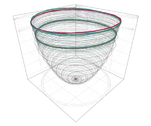
Figure 1. Encoder–decoder procedure: (a) obtaining flow field snapshots from simulations or experiments; (b) encoder part, representing the Isomap method application on input snapshots to identify the embedding manifold in low-dimensional space; (c) decoder part which reconstruct the flow field snapshots from low-dimensional space coordinates.
Let us consider that  $N$ flow field snapshots have been observed, either from an experimental setting or a simulation. Considering that each snapshot is a matrix of
  $P$ elements, the vectorized version of each snapshot is an observation (point) in the high-dimensional space
  $\mathbb {R}^P$, where each dimension (feature) contains information about a point of the field. Let
  $\boldsymbol{\mathsf{X}}\in {\mathbb {R}}^{N\times P}$ be the data matrix containing the stated information and
  $\boldsymbol {x}_i\in \mathbb {R}^P$ be each of its rows, i.e. the flow fields for
  $i=1,\ldots,N.$ The dataset in
  $\boldsymbol{\mathsf{X}}$ is complex by nature and being able to extract a meaningful small number of coordinates that capture the main characteristics of the flow is challenging.
Isometric feature mapping is a nonlinear dimensionality reduction technique that finds a low-dimensional embedding of the data points that best preserve the geodesic distances measured in the high-dimensional input space. In order to estimate these geodesic distances, the shortest paths in a graph-connecting neighbouring points are employed. These distances are then used as an input in classical MDS (Torgerson Reference Torgerson1952) to construct the low-dimensional embedding so that the Euclidean pairwise distances resemble those in the neighbouring graph. Therefore, the Isomap algorithm runs as follows. First, the Euclidean distances  $d_{\boldsymbol{\mathsf{X}}}(i,j)$ between flow fields
  $\boldsymbol {x}_i$ and
  $\boldsymbol {x}_j$, corresponding to the
  $i{\rm th}$ and
  $j{\rm th}$ rows of
  $\boldsymbol{\mathsf{X}}$, are computed for all
  $i,j=1,\ldots,N$. Second, for
  $i=1,\ldots,N$,
  $\mathcal {N}_{\boldsymbol{\mathsf{X}}}^k(i),$ is defined as the set of the
  $k$ closest observations to
  $\boldsymbol {x}_i.$ Based on these neighbourhoods, the neighbouring graph
  $\boldsymbol{\mathsf{G}}$ is defined over these data points such that two nodes (flow fields)
  $i$ and
  $j$ are connected by an edge of weight
  $d_{\boldsymbol{\mathsf{X}}}(i,j)$ if they are neighbours, i.e. there is an edge between
  $i$ and
  $j$ if
  $\boldsymbol {x}_j\in \mathcal {N}_{\boldsymbol{\mathsf{X}}}(i)$. Observe that
  $\boldsymbol{\mathsf{G}}$ approximates the high-dimensional manifold containing the observed data. See Appendix A for a discussion about the choice of the number of neighbours
  $k$ to build
  $\boldsymbol{\mathsf{G}}$. Third, the shortest paths between all pair of vertices in
  $\boldsymbol{\mathsf{G}}$ are computed, yielding
  $d_{\boldsymbol{\mathsf{G}}}(i,j)$ for all
  $i,j=1,\ldots,N$, using Floyd's algorithm (Floyd Reference Floyd1962). Let
  $\boldsymbol{\mathsf{D}}_{\boldsymbol{\mathsf{G}}}$ be the matrix containing these shortest path distances. Finally, obtain the low-dimensional embedding
  $\boldsymbol {\varGamma }\in {\mathbb {R}}^{N\times p},$
  $p\ll P$, using MDS. The new coordinates for the
  $N$ samples are then found so that their pairwise Euclidean distance resembles
  $d_{\boldsymbol{\mathsf{G}}}(i,j)$. This is equivalent to finding
  $\boldsymbol {\varGamma }$ which minimizes the cost function
 \begin{equation} \left\Vert \boldsymbol{\varGamma\varGamma}^\top - \boldsymbol{\mathsf{B}}\right\Vert_F^2, \end{equation}
where  $\boldsymbol{\mathsf{B}} = -\frac {1}{2}\boldsymbol{\mathsf{H}}^\top (\boldsymbol{\mathsf{D}}_{\boldsymbol{\mathsf{G}}} \odot \boldsymbol{\mathsf{D}}_{\boldsymbol{\mathsf{G}}})\boldsymbol{\mathsf{H}}$ is the Gram matrix in the input space, with
  $\boldsymbol{\mathsf{H}}= \boldsymbol{\mathsf{I}}_N - ({1}/{N})\mathbb {1}_N$ being the centring matrix,
  $\boldsymbol{\mathsf{I}}_N$ the identity matrix of dimension
  $N$,
$N$,  $\mathbb {1}_N$ the all-ones matrix of dimension
  $N$,
$N$,  $\odot$ the Hadamard (element-wise) product and
  $\|{\cdot }\|_F$ the Frobenius norm.
Fixing a dimension  $p$ for the low-dimensional embedding, the value of
  $\boldsymbol {\varGamma }$ minimizing the quantity in (2.1) is the matrix made up of the
  $p$ eigenvectors
  $\boldsymbol {\gamma }_1,\ldots,\boldsymbol {\gamma }_p$ corresponding to the
  $p$ largest (positive) eigenvalues of the matrix
  $\boldsymbol {\varLambda }$ arising from the eigendecomposition of
  $\boldsymbol{\mathsf{B}}$, namely
  $\boldsymbol{\mathsf{B}} = \boldsymbol{\mathsf{V}}\boldsymbol{\varLambda}\boldsymbol{\mathsf{V}}^\top$ and
  $\boldsymbol {\varGamma } = \boldsymbol{\mathsf{V}}_p.$
The aforementioned Isomap algorithm admits the choice of other norms different from the Euclidean, different ways of identifying the neighbours to construct  $\boldsymbol{\mathsf{G}}$, other shortest path algorithms or a non-classical approach to MDS. However, the choices made in our methodology are motivated by the implemented version of Isomap in the RDRToolbox in the R software (R Core Team 2020; Bartenhagen Reference Bartenhagen2021), which has been used to carry out our analyses.
In order to assess the performance of Isomap, Tenenbaum et al. (Reference Tenenbaum, de Silva and Langford2000) proposed using the definition of residual variance as in (2.2). Let  $\boldsymbol{\mathsf{D}}_{\boldsymbol {\varGamma }}$ be the matrix of Euclidean distances between each pair of points in the low-dimensional embedding. Then, the residual variance is defined as one minus the squared correlation coefficient between the vectorization of the distance matrices
  $\boldsymbol{\mathsf{D}}_{\boldsymbol{\mathsf{G}}}$ and
  $\boldsymbol{\mathsf{D}}_{\boldsymbol {\varGamma }}$, yielding
 \begin{equation} 1- R^2(\text{vec}\left(\boldsymbol{\mathsf{D}}_{\boldsymbol{\mathsf{G}}}\right), \text{vec}\left(\boldsymbol{\mathsf{D}}_{\boldsymbol{\varGamma}}\right)), \end{equation}
where  $R^2$ refers to the squared correlation coefficient and ‘vec’ is the vectorization operator. Observe that the result in (2.2) is a number between
  $0$ and
  $1$ which accounts for the amount of information that remains unexplained by the low-dimensional embedding of the original data. Therefore, the lower the value in (2.2) the better. For a discussion about the definition of residual variance to assess the performance of Isomap against other dimensionality-reduction methods such as POD we refer the reader to Appendix B.
In order to provide a decoder to create a correspondence between Isomap coordinates  ${\gamma}_1,\ldots,{\gamma}_p$ and the ones in the high-dimensional space, namely
  $\mathbb {R}^P,$ we employ a purely data-driven approach. Any flow field
  $\boldsymbol {x}_i\in \mathbb {R}^P$ has its low-dimensional counterpart
  $\boldsymbol {y}_i\in \mathbb {R}^p$,
  $i=1,\ldots,N.$ Then, let
  $f:\mathbb {R}^p\longrightarrow \mathbb {R}^P$ be the unknown mapping which transforms the flow fields in the low-dimensional space onto the high-dimensional ones. To reconstruct the flow field for any
  $\boldsymbol {y}\in \mathbb {R}^p$ we assume that its
  $K$-nearest neighbours
  $\boldsymbol {y}_{(1)},\ldots, \boldsymbol {y}_{(K)}$ and their high-dimensional counterparts, namely
  $\boldsymbol {x}_{(1)},\ldots, \boldsymbol {x}_{(K)},$ are identified. Therefore, the reconstruction (or decoding) of
  $\boldsymbol {y},$ denoted as
  $\boldsymbol {x},$ can be obtained as a first-order Taylor expansion starting from the nearest neighbour to be mapped back to the original space, i.e.
  $\boldsymbol {x}_{(1)},$ as
 \begin{equation} \boldsymbol{x} = \boldsymbol{x}_{(1)} + (\boldsymbol{y} - \boldsymbol{y}_{(1)}) \boldsymbol{\nabla} f(\boldsymbol{y}_{(1)})^\top, \end{equation}
where the gradient tensor in  $\boldsymbol {y}_{(1)}$, namely
  $\boldsymbol {\nabla } f(\boldsymbol {y}_{(1)})=({\partial f}/{\partial {\gamma_1}}(\boldsymbol {y}_{(1)}),\ldots, {\partial f}/{\partial {\gamma _p}}(\boldsymbol {y}_{(1)}))$ is estimated assuming an orthogonal projection of the
  $K-1$ directions provided by the
  $K$-nearest neighbours in
  $\mathbb {R}^P$ to those in
  $\mathbb {R}^p.$ This is
 \begin{equation} \begin{bmatrix} \boldsymbol{x}_{(2)} - \boldsymbol{x}_{(1)}\\ \ldots \\ \boldsymbol{x}_{(K)} - \boldsymbol{x}_{(1)} \end{bmatrix} \simeq \begin{bmatrix} \boldsymbol{y}_{(2)} - \boldsymbol{y}_{(1)}\\ \ldots \\ \boldsymbol{y}_{(K)} - \boldsymbol{y}_{(1)} \end{bmatrix}\boldsymbol{\nabla} f(\boldsymbol{y}_{(1)})^\top, \end{equation}
which yields  $\boldsymbol {\nabla } f(\boldsymbol{y}_{(1)})^\top = (\Delta \boldsymbol{\mathsf{Y}}^\top \Delta \boldsymbol{\mathsf{Y}})^{-1}\Delta \boldsymbol{\mathsf{Y}}^\top \Delta \boldsymbol{\mathsf{X}}$ if least squares minimization is used to approximate it, and
  $\Delta \boldsymbol{\mathsf{X}}$ and
  $\Delta \boldsymbol{\mathsf{Y}}$ are the left-hand side and the first term in the right-hand side of (2.4), respectively.
3. Datasets
In this section we describe the datasets that have been used to test our methodology. Three configurations are considered, which yield different flow fields and regimes under both experimental and simulation set-ups.
3.1. Fluidic pinball dataset
The fluidic pinball is a flow configuration consisting of three rotatable cylinders of equal diameter  $D$ whose axes are located in the vertices of an equilateral triangle, as sketched in figure 2(a). The triangle has a centre-to-centre side length
  $3D/2$ and is immersed in a viscous incompressible flow with a uniform upstream velocity
  $U_\infty$. The Reynolds number for this set-up is defined as
  $Re = U_\infty D/\nu$, where
  $\nu$ is the kinematic viscosity of the fluid. The wake flow undergoes a set of interesting transitions at different values of the Reynolds number. This allows exploration of reduced-order modelling and flow control strategies in a wide range of scenarios. In the recently published literature, the fluidic pinball has been used as a benchmark configuration for testing the mean-field modelling (Deng et al. Reference Deng, Noack, Morzyński and Pastur2020), cluster-based network modelling (Deng et al. Reference Deng, Noack, Morzyński and Pastur2022) and machine learning control (Raibaudo et al. Reference Raibaudo, Zhong, Noack and Martinuzzi2020; Cornejo Maceda et al. Reference Cornejo Maceda, Li, Lusseyran, Morzyński and Noack2021).
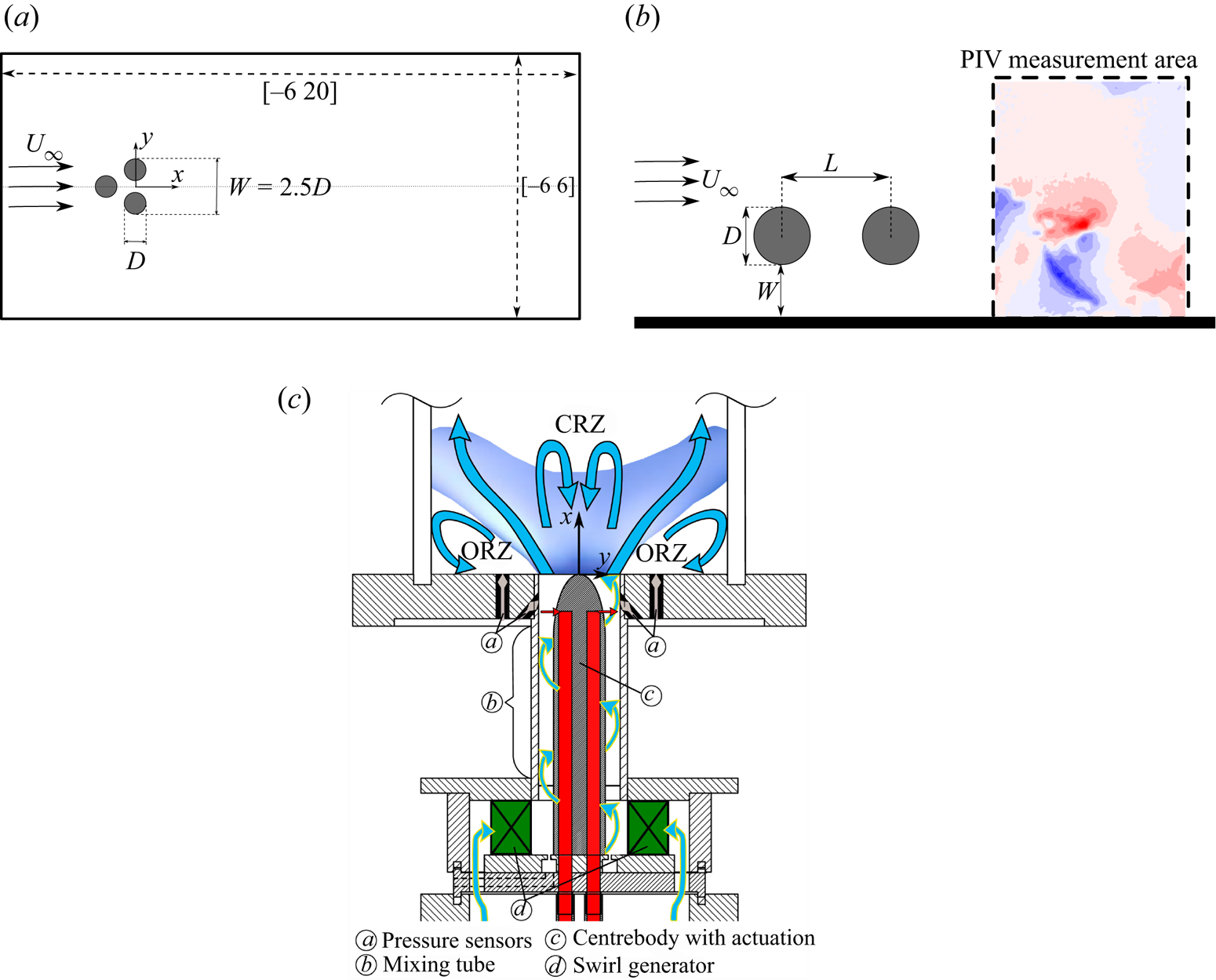
Figure 2. Dataset configurations: (a) fluidic pinball; (b) tandem cylinders; (c) swirling jet (Reprinted from Lückoff et al. (Reference Lückoff, Kaiser, Paschereit and Oberleithner2021) with permission from Elsevier).
The numerical results of the fluidic pinball are investigated by employing a software developed to study multiple-input multiple-output flow control by Noack & Morzyński (Reference Noack and Morzyński2017). Direct numerical simulations of the non-dimensionalized incompressible Navier–Stokes equations are used to compute the two-dimensional viscous wake behind the pinball configuration, where the variables are scaled with length  $D$, velocity
  $U_\infty$, time
  $D/U_\infty$ and density
  $\rho$. As shown in figure 2(a), the computational domain
  $[-6D,20D] \times [-6D,6D]$, excluding the interior of the cylinders, is described by a Cartesian coordinate system whose origin is located in the middle of the rear cylinders. As the rotation of the cylinders is not considered in this study, a no-slip condition on the cylinders, the far-field velocity
  $U_\infty$ and a no-stress condition applied at the outlet of the domain are considered as the boundary conditions. The unsteady Navier–Stokes solver is based on third-order fully implicit time integration using an iterative Newton–Raphson approach and second-order finite-element method discretization on an irregular grid structure with 4225 T6 triangles and 8633 vertices (Deng et al. Reference Deng, Noack, Morzyński and Pastur2020). In order to simplify the distance calculation between snapshots, data is interpolated on a high-resolution uniform grid containing a total of 77 679 points. The steady solution, used as the initial condition at each corresponding Reynolds number, is calculated by the solver for the steady Navier–Stokes equations in the same way. In figures 3(a) and 3(b), the fluctuating streamwise and crosswise velocity field of an example snapshot at
  $Re=130$ are shown after subtracting the symmetric steady solution.
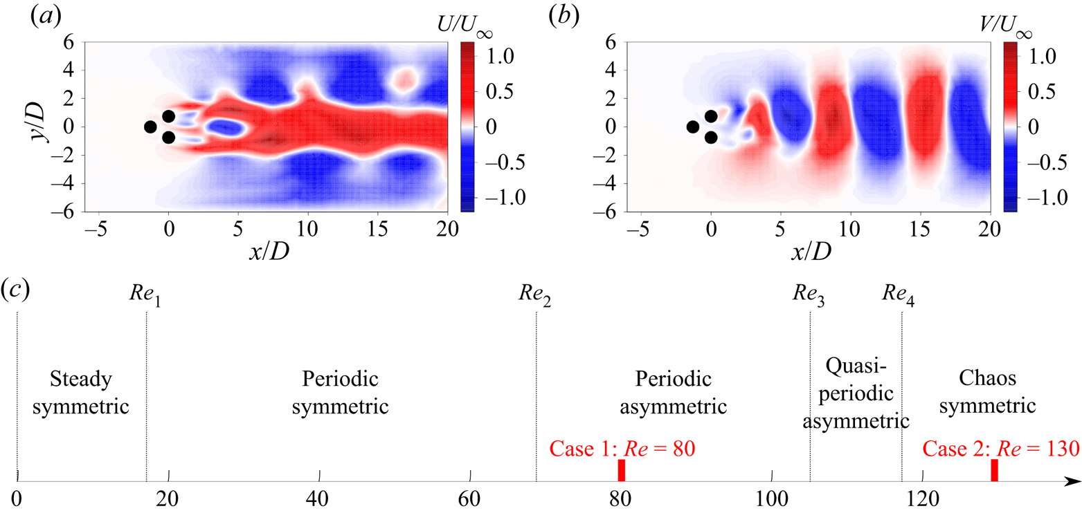
Figure 3. An example snapshot of the fluidic pinball at  $Re=130$ after subtracting the steady solution: (a) the contour of the streamwise fluctuating velocity component U; and (b) the contour of the crosswise fluctuating velocity component V, normalized with the upstream velocity
  $U_\infty$. (c) Transitions of different flow regimes with varying Reynolds numbers.
With increasing Reynolds number, the flow experiences a transition from a laminar flow to periodic vortex shedding and finally to chaos (Deng et al. Reference Deng, Noack, Morzyński and Pastur2020). Five different regimes have been identified, as summarized in figure 3(c). The transition from a steady symmetric flow to a periodic symmetric vortex shedding occurs at  $Re_1 \approx 18$ (following a Hopf bifurcation (Andronov et al. Reference Andronov, Leontovich, Gordon and Maier1971; Strogatz et al. Reference Strogatz, Friedman, Mallinckrodt and McKay1994)). The symmetry of the vortex shedding vanishes at
  $Re_2 \approx 68$ (pitchfork bifurcation (Strogatz et al. Reference Strogatz, Friedman, Mallinckrodt and McKay1994)) thus entering a periodic asymmetric regime, presenting as an asymmetric vortex shedding with the base-bleeding jet deflected upward or downward. A secondary frequency appears with a higher Reynolds number, and the flow experiences another transition to a quasiperiodic asymmetric regime at
  $Re_3 \approx 104$ (Neimark–Säcker bifurcation (Kuznetsov & Sacker Reference Kuznetsov and Sacker2008)), where the jet oscillates with the lower frequency. Finally, at
  $Re_4 \approx 115$, the flow enters into a chaotic symmetric regime with the jet oscillating randomly.
In this study, we focused on two different flow states at the selected  $Re$, representative of the two most complex flow states identified by Deng et al. (Reference Deng, Noack, Morzyński and Pastur2022). At
  $Re=80$ for the periodic asymmetric regime, there exist a total of six invariant sets in the system state space: three unstable steady solutions; one unstable limit cycle; and two stable limit cycles, resulting from the primary Hopf bifurcation and the secondary pitchfork bifurcation. The unsteady flow is continuously sampled into snapshots with a fixed time step equal to
  $0.1$. A time horizon is chosen long enough to ensure the flow data contain the transient and post-transient dynamics from the unstable steady state to the asymptotic state. The dataset at
  $Re=80$ includes the snapshots from the simulations starting from the symmetric steady solution and its mirror-conjugated snapshots for a time horizon of 1500, as well as the snapshots from the simulations starting from the two mirror-conjugated asymmetric steady solutions for a time horizon of 1000. In this case, it is able to ensure that the dataset contains the complete manifold with six invariant sets. At
  $Re=130$ for the chaotic symmetric regime, three unstable steady solutions and one chaotic attracting set can be found. The dataset considered at
  $Re=130$ only contains the snapshots from the simulation starting from the symmetric steady solution for a time horizon of 1500, since we are interested in the transition from the unstable invariant set to the chaotic attracting set in this case. For the present analysis we limited the total number of snapshots to be analysed to 4000 for both Reynolds numbers. Snapshots are selected homogeneously from the whole range of the simulation covering complete evolution of the flow field until the final limit cycles. Therefore, simulations are performed at
  $Re$ equal to
  $80$ and
  $130$, thus covering the typical complex wake dynamics regime with multiple invariant sets and chaotic attracting set.
3.2. Swirling jet dataset
Swirling jets have a wide variety of applications in modern gas turbine combustors and aerodynamically stabilize lean premixed flames. In the present work we analyse an experimental dataset obtained with stereoscopic PIV by Lückoff et al. (Reference Lückoff, Kaiser, Paschereit and Oberleithner2021). Figure 2(c) shows a schematic of the swirling nozzle and of the measurement domain employed in the work by Lückoff et al. (Reference Lückoff, Kaiser, Paschereit and Oberleithner2021). This configuration consists of a feeding line which provides the mass flow rate to a jet issued from a swirling nozzle. The swirling flow is produced using a radial swirl generator and the swirl number  $Sw$, defined as the ratio of the axial flux of tangential momentum to the axial flux of axial momentum, can range between 0 and 1.5. The nozzle exit has a diameter of
  $D = 55\ {\rm mm}$ and has a centrebody at the centre with diameter
  $D_{CB} = 35\ {\rm mm}$ thus the hydraulic diameter of the mixing tube has a diameter of
  $D_h = 20\ {\rm mm}$. The Reynolds number is defined using the hydraulic diameter and the experimental facility can provide jets with a Reynolds number in the range
  $[13\,000, 32\,000]$. The present dataset has been generated for
  $Re = 20\,000$ and
  $Sw = 0.7$.
The measurement domain is located at the nozzle exit to analyse the flow in the combustion chamber. The combustion chamber is a cylinder with an inner diameter of  $D_{CCh} = 200\ {\rm mm}$ and a length of
  $L_{CCh} = 300\ {\rm mm}$ and is made of quartz glass to enable flow measurement using time-resolved stereoscopic PIV. For the present dataset, 2183 snapshots were captured at a frame rate of 2500 f.p.s. The stereoscopic PIV system consists of a Nd:YLF diode pumped laser, which is synchronized with two high-speed CMOS cameras at
  $1024 \times 1024$ pixels image resolution. One camera was mounted perpendicular to the streamwise field of view and one was mounted with an angle of
  $40^{\circ }$ to the measurement plane. The two camera views were aligned using a multilevel calibration target. A laser light sheet of approximately 1 mm thickness was generated to illuminate the measurement area. For PIV seeding, heat-resistant solid titanium dioxide (
 ${\rm TiO}_{2}$) particles of a nominal diameter of
  $2\ \mathrm {\mu } {\rm m}$ were introduced to the flow far upstream using a brush-based seeding generator. The acquired particle snapshots were processed using a commercial PIV software which employs a correlation scheme with multigrid refinement. The final window size was set to
  $16\times 16$ pixels with an overlap of
  $50\,\%$ in combination with spline-based image deformation and subpixel peak fitting. Finally, the estimated velocity fields were filtered for removing outliers, which were always less than 1 %. The velocity at the actuators outlet has been measured using hot-wire sensors. The reader can refer to the work by Lückoff et al. (Reference Lückoff, Kaiser, Paschereit and Oberleithner2021) for further details on the measurement set-up and PIV image processing.
The main coherent structure in this kind of flow is a helical structure known as the precessing vortex core (PVC) (Syred Reference Syred2006), which is generated due to a global self-excited instability (Müller et al. Reference Müller, Lückoff, Paredes, Theofilis and Oberleithner2020). Although the origin of the PVC is well understood, its impact on combustion performance, especially flame stability, is still a matter for study. The existence of a dominant coherent structure in this flow encourages the idea that manifold learning can be successfully implemented to study the behaviour of the PVC under different conditions.
3.3. Tandem cylinders dataset
The third dataset employed in this work consists of flow field measurements in the wake of tandem cylinders near a wall. The data refer to the work by Raiola et al. (Reference Raiola, Ianiro and Discetti2016); the experimental configuration is summarized here for completeness. As sketched in figure 2(b), this configuration consists of two equal cylinders located in a cross-flow which are separated by a ratio of  $L/D$ denoted as the longitudinal pitch ratio (with
  $L$ being the longitudinal distance between two cylinders centres and
  $D$ the diameter of the cylinders equal to
  $32\ {\rm mm}$). Both cylinders are placed at a similar distance to a wall with a ratio of
  $W/D$ denoted as the wall gap ratio (with
  $W$ being the distance of the cylinders from the wall). The wind-tunnel velocity
  $U_\infty$ is set constant and equal to
  $2.3\ {\rm m}\ {\rm s}^{-1}$ in order to achieve a Reynolds number of
  $4900$, based on cylinder diameter (Raiola et al. Reference Raiola, Ianiro and Discetti2016). In this study, the longitudinal pitch ratio is set to
  $L/D=1.5$ and the wall gap ratio is set to
  $W/D=3$.
An ensemble of 1800 flow field snapshots is employed for the present study. Velocity field measurements are performed with digital planar PIV. Di-ethyl-hexyl-sebacate (DEHS) droplets of approximately  $1\ \mathrm {\mu } {\rm m}$ diameter are employed to seed the flow. The acquisition is performed at
  $10\ {\rm Hz}$ with a TSI PowerViewTM Plus 2MP Camera (with an array of
  $1600\times 1200$ pixels) with a spatial resolution of approximately
  $7.2\ {\rm pixels}\ {\rm mm}^{-1}$. The light source employed is a Big Sky Laser CFR400 ND:Yag (
 $230\ {\rm mJ}\ {\rm pulse}^{-1}$, pulse duration
  $3\ {\rm ns}$). Image quality is improved by removing laser reflections and illumination background (Mendez et al. Reference Mendez, Raiola, Masullo, Discetti, Ianiro, Theunissen and Buchlin2017). The interrogation strategy employed is an iterative multistep (Soria Reference Soria1996) image deformation (Scarano Reference Scarano2001) algorithm, with a final interrogation window size of
  $16\times 16$ pixels, with 50 % overlap resulting in a final vector spacing of approximately
  $0.035D$. Outlier vectors are identified with the universal median test by Westerweel & Scarano (Reference Westerweel and Scarano2005) on a
  $3\times 3$ vector kernel using a threshold equal to 2. Outliers are replaced with a distance-weighted average of valid neighbours.
While Raiola et al. (Reference Raiola, Ianiro and Discetti2016) reported that a gap ratio of  $W/D=3$ is sufficient to have negligible wall-interaction effects, three main flow behaviours in the wake of tandem cylinders can be identified based on the Reynolds number and the distances between the two cylinders. Zdravkovich (Reference Zdravkovich1997) classified the flow around tandem cylinders with identical diameters into three major regimes (extended body; reattachment; and coshedding), depending on the longitudinal pitch ratio. At low longitudinal distance (
 $L/D<1.5$), the vortex shedding for the upstream cylinder is suppressed, and the system acts as a unified bluff-body, which is categorized as the extended body regime or single bluff-body regime. By increasing the longitudinal distance (
 $1.5< L/D<4$), the flow starts to show a more complex behaviour which mainly can be characterized by the reattachment of the separated free shear layers from the upstream cylinder on the surface of the downstream cylinder. This regime is referred to as the ‘reattachment’ regime. Furthermore, by increasing the longitudinal distance, both cylinders feature the typical characteristics of the von Kármán vortex street. This regime is often defined the ‘coshedding’ regime. Alam et al. (Reference Alam, Elhimer, Wang, Lo Jacono and Wong2018) report the existence of a transitional
  $L/D$ range between the reattachment and coshedding regimes also referred to as ‘critical’ or ‘bistable’ flow spacing. While it can be argued that a similar bistable regime should occur also between the extended body and the reattachment regimes, Raiola et al. (Reference Raiola, Ianiro and Discetti2016) did not identify such a feature for
  $L/D=1.5$. This dataset appears to be especially suited to discover whether nonlinear manifold learning could unveil such a kind of bistable regime.
4. Results
This section presents and discusses the performance of the proposed encoder–decoder algorithm. The first subsection is dedicated to the performance of the encoder part. We discuss its strengths in unravelling the physical characteristics of the flows distilling the manifolds. In the second subsection, the decoder's ability to reconstruct the original flow fields from the obtained low-dimensional coordinates is analysed.
4.1. Encoder's capabilities
In this section, the embedding manifolds obtained from Isomap are presented for the datasets described in § 3.
In order to compute the dimensionality of the datasets at hand, the residual variance as defined in (2.2) is obtained for each number of dimensions. The choice of  $p$ is then made based on the elbow method following Tenenbaum et al. (Reference Tenenbaum, de Silva and Langford2000). The dimension beyond which the residual variance experiences negligible variation can be identified as the true dimensionality of the dataset. This method is also widely used to compute the proper number of the clusters in the clustering techniques (Kaufman & Rousseeuw Reference Kaufman and Rousseeuw1990). The ‘true’ dimensionality is the proper place in a trade-off between the simplicity of the embedded manifold and the loss of information due to truncation.
An example of residual variance as a function of the number of selected dimensions is reported in figure 4(a) for the case of the wake of the pinball at  $Re = 80$ and
  $Re = 130$. For the lowest Reynolds number, it can be seen that three dimensions are sufficient to describe the bulk of the variance since the resulting residual variance for dimensions higher than three remains approximately the same. Note that due to its definition, the residual variance might not be monotonically decreasing with an increasing number of coordinates; for more details the reader is referred to Appendix B. On the other hand, truncating at three dimensions at
  $Re=130$ appears to still be acceptable although it induces a larger error in terms of explained variance.
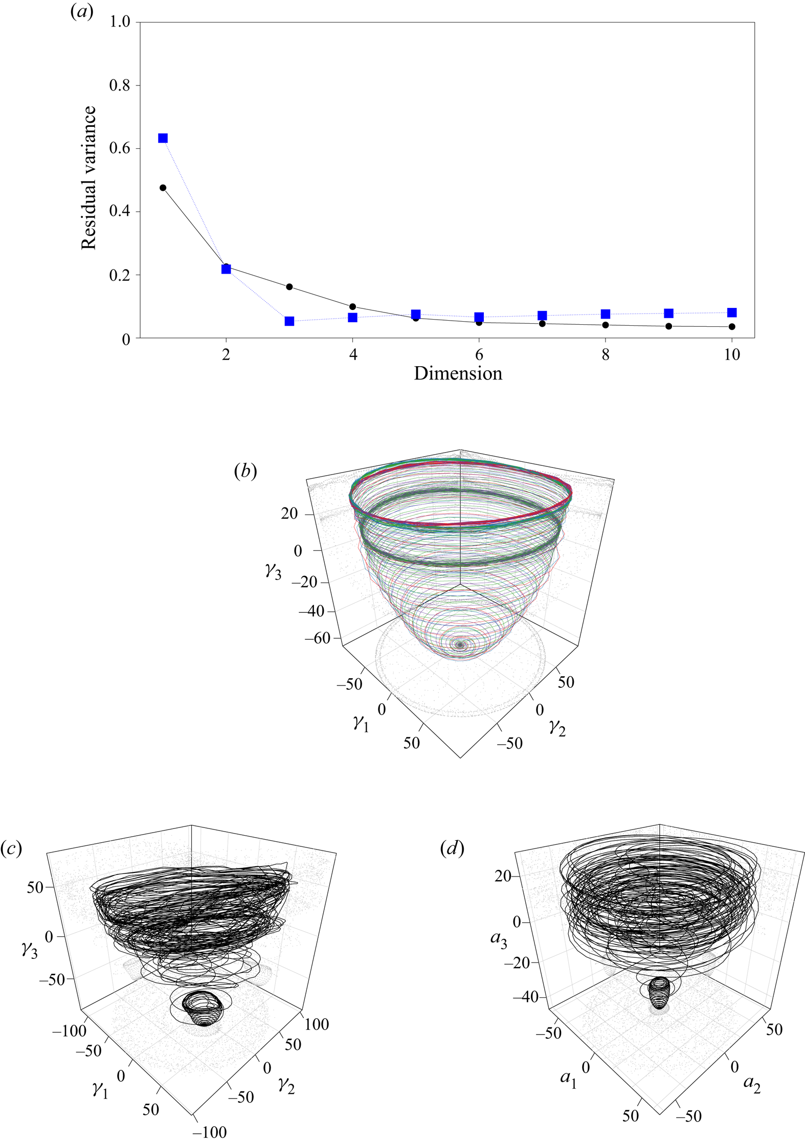
Figure 4. Isomap and POD results for the pinball datasets. (a) Residual Variance: blue,  $Re = 80$; black,
  $Re = 130$. (b) Perspective view of the Isomap embedded manifold of
  $Re = 80$: purple, symmetric steady solution; green, flipped symmetric steady solution; red, asymmetric upward steady solution; blue, asymmetric downward steady solution. (c) Perspective view of the Isomap embedded manifold of
  $Re = 130$. (d) Perspective view of the POD embedded manifold of
  $Re = 130$.
It must be remarked that, from now on, we are limited in plotting the projection of the manifold on the first three dimensions; nonetheless, the number of dimensions needed to represent accurately the manifold might be larger, depending on the complexity of the dynamics.
4.1.1. Fluidic pinball
Figure 4(a) shows the residual variances of the pinball configuration dataset for  $Re = 80$ (blue) and
  $p=1,\ldots,10$. For this configuration, the chosen value of
  $k$ is equal to 8; for more details about the choice of
  $k$ the reader is referred to Appendix A. The elbow is attained for
  $p=3$ which is considered to be the true dimensionality of this problem. The residual variance is approximately the same for
  $p>3$, thus, it can be argued that the manifold of input data, embedded in a higher-dimensional state space, has three key dimensions.
The same procedure has been done for the  $Re = 130$ case, employing
  $k=12$. The residual variance (see the black curve in figure 4a) decreases monotonically for an increasing number of dimensions and is already below 20 % after three-dimensions (
 $p=3$). However, the residual variance value at
  $p=3$ increases by increasing the Reynolds number to higher values and entering the more chaotic regimes. This indicates that in the chaotic regime the ‘true’ dimensionality is higher due to the arising of a more complex dynamics. Therefore, it is reasonable to expect that, for increasing Reynolds number, the number of dimensions needed to explain the bulk of the variance should increase. This behaviour is not surprising, and it is observed in virtually all dimensionality-reduction techniques.
In terms of manifold shape, both for  $Re = 80$ and
  $130$, the data lies on a paraboloid (figures 4b and 4c accordingly) with the first two coordinates (
 $\gamma _1$ and
  $\gamma _2$) being representative of the periodic vortex shedding and the third coordinate being representative of a shift-mode characteristic of the transient dynamics from the onset of vortex shedding to the periodic von Kármán wake, analogously to what was found for the cylinder wake by Noack et al. (Reference Noack, Afanasiev, Morzyński, Tadmor and Thiele2003). A similar paraboloid shape is reported for the fluidic pinball at
  $Re=30$ by Deng et al. (Reference Deng, Noack, Morzyński and Pastur2020). It is remarkable that, when analysing all the solutions at
  $Re=80$, the manifold correctly identifies the first unstable limit cycle for the symmetric unsteady solution and is able to identify the differences between the asymmetric upward and downward limit cycle. As well for
  $Re=130$, the chaotic nature of the data shows a less smooth manifold, which still reveals the characteristic paraboloid shape. When employing POD and plotting the first three temporal modes, similar shapes could be obtained although less clear, especially at
  $Re=130$, as evident from the comparison of figures 4(c) and 4(d). Plotting the POD results at
  $Re=80$, the resulting manifold shows a similar behaviour as depicted in figure 4(b) and thus it is omitted for the sake of brevity.
Although the dimensions identified by Isomap do not necessarily have a physical meaning, it is a useful exercise to establish whether there exists some correlation between such coordinates and relevant flow quantities. Figure 5(a) shows a clear correlation between the drag coefficient and the coordinate  $\gamma _3$. This correlation is expected, since we observed that the third coordinate is representative of the shift mode. Some pairs of coordinates are related to higher-order harmonics of the flow, as is the case for
  $\gamma _1 - \gamma _2$,
  $\gamma _4 - \gamma _5$, and
  $\gamma _6 - \gamma _7$. Interestingly enough, if we extend the analysis to higher-order coordinates, it is possible to identify a high degree of correlation between the
  $\gamma _8$ and the lift coefficient
  $C_L$, as shown in figure 5(b). Although these interpretations are case-sensitive and can be affected by changes in the flow configuration and starting conditions in the Isomap algorithm, we have identified situations in which some coordinates in the low-dimensional space could be related to the main flow features. While it is outside of the scope of this paper to assess the interpretability of the coordinates identified by Isomap, we spotlight the possibility of the existence of such a kind of correlation. This could be a powerful catalyst for the extension of the encoder–decoder framework presented here, and it will be object of future study.
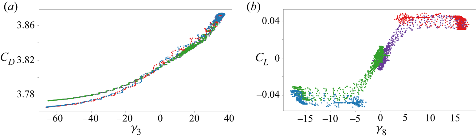
Figure 5. Relation between the coordinates of the embedded manifold and the force coefficients for the fluidic pinball at  $Re=80$: (a) the drag coefficient (
 $C_D$) versus third coordinate; (b) the lift coefficient (
 $C_L$) versus eighth coordinate; purple, symmetric steady solution; green, flipped symmetric steady solution; red, asymmetric upward steady solution; blue, asymmetric downward steady solution.
4.1.2. Swirling jet
In the more challenging experimental case of the swirling jet, the same encoder procedure based on Isomap using  $k = 8$ has been carried out. Here POD and Isomap performance as encoders is compared.
Figure 6(a) shows the residual variances of Isomap (black dots) and POD (green triangles), which is measured as stated in Appendix B, for different numbers of dimensions. In this case, the values of residual variance are significantly larger compared with those in the simulation cases studied before, most likely due to the turbulent nature of the flow and possibly due to measurement noise in the experimental data. It is worth noting that the residual variances of Isomap are lower than those of POD for all the dimensions depicted, thus indicating that Isomap is a better manifold learner in this case to preserve the geometry of the high-dimensional dataset. To investigate this advantage, we can compare the resulting embedding in both cases for three dimensions, which accounts for a reasonable amount of residual variance. Figures 6(b) and 6(d) show the encoded data by Isomap, whereas figures 6(c) and 6(e) illustrate the POD results, respectively. Although for both methods the general shape of the embedded manifold is similar to a hollow cylinder, the one obtained by Isomap shows a more clearly defined shape. Furthermore, the diameter of the hollow cylinder in POD is smaller and less circular with more spread points. Thus, the Isomap encoding provides a more helpful base to interpret the manifold and eventually relate the low-dimensional coordinates to the physical features of the flow.

Figure 6. Resulted manifold from Isomap and POD for the swirling jet case. (a) Residual variance: green, POD; black, Isomap. (b) Three-dimensional Isomap. (c) Three-dimensional POD. (d) Top view, Isomap. (e) Top view, POD.
4.1.3. Tandem cylinders
Regarding the tandem cylinder dataset, figure 7(a) shows that an appropriate number of dimensions in terms of the residual variance for both Isomap (black dots) and POD (green triangles) is two. Furthermore, as in the previous case, Isomap outperforms POD in terms of residual variance. As in the swirling-jet case discussed above, the Isomap results in figure 7(b) show a clearer manifold compared with the one obtained by POD (figure 7c). Furthermore, it also shows some separate groups of snapshots related to some physical features of the flow while the manifold resulted from POD ultimately fails to capture this behaviour of the system. Setting the number of groups to three, the results of the classification in the polar coordinates are shown by means of different colours in figure 7(b). The flow fields of each group close to the  $\gamma _1=0$ line are plotted in figures 7(d)–7( f) from the outer group (Group 1) to the inner one (Group 3), as the representative of each group. We investigate each group by looking at these representative snapshots, which are highlighted with larger, numbered symbols in figure 7(b). As we move outward from the centre (
 $\gamma _1=\gamma _2=0$), the distance between two consecutive vortices in the wake decreases, and the vortices appear less intense. In other words, moving from the groups from the outer part to the inner one, a transition between two different vortex shedding regimes is found which is conjectured to correspond to the bluff-body regime and the reattachment regime of the tandem cylinders. As described in § 3.3, previous studies suggest that this configuration of the flow lies on the bluff-body regime, as most of the snapshots in the low-dimensional space classify in the outer and middle groups, and the results of our encoding procedure are consistent with previous studies done by using POD (Raiola et al. Reference Raiola, Ianiro and Discetti2016). However, Isomap can capture that even in this configuration, some behaviour of the next regime can coexist with the dominant one, suggesting that we cannot define a specific number for
  $L/D$ as the classifier of the flow regimes, and by increasing
  $L/D$ the flow smoothly changes its behaviours.

Figure 7. Resulted manifold from Isomap and POD for the tandem cylinders case. (a) Residual variance: green, POD; black, Isomap. (b) Isomap grouped embedding manifold: red, Group 1; black, Group 2; blue, Group 3. (c) Proper orthogonal decomposition. (d–f) Sample snapshots for Groups 1, 2 and 3 corresponding to the points labelled as 1, 2 and 3 on the manifold in panel (b).
4.2. Decoder's performance
This section assesses the quality of the decoder approach described in § 2. The normalized mean squared error (NMSE) in a test set of observations  $\mathcal {T}$ is computed as
 \begin{equation} NMSE = \frac{1}{|\mathcal{T}|}\sum_{\boldsymbol{x}\in\mathcal{T}} \frac{\|\boldsymbol{x} - \hat{\boldsymbol{x}}\|^2}{\|\boldsymbol{x}\|^2}, \end{equation}
where  $\hat {\boldsymbol {x}}$ is the decoder's reconstruction of the flow field
  $\boldsymbol {x}\in \mathbb {R}^P$.
Table 1 shows the average NMSE obtained for the different cases studied (last column), namely pinball for  $Re = 80$ and
  $Re = 130$, the swirling jet flow and the wake of tandem cylinders. The sample data has been split into
  $70\,\%$ training and
  $30\,\%$ testing. The number of neighbours considered in Isomap (
 $k$) and the number of neighbours considered in the decoding stage (
 $K$) are reported in the sixth and seventh columns, respectively. The first column in table 1 depicts the case study, the second the value of
  $Re$, the third the number of samples, fourth the number of features in the high-dimensional space and fifth the number of dimensions considered for Isomap. Note that the NMSEs reported in table 1 are actually representation errors, i.e. the error incurred when reconstructing the original datasets by means of our encoder–decoder methodology. These representation errors show that the decoder has an excellent performance on the simulation datasets and has a reasonably good performance on both turbulent experimental datasets. Figure 8 compares reconstructed and actual snapshots for a random point in the test subset. As expected from the reported errors, the differences between the two snapshots in the pinball case are hardly noticeable. In the case of the tandem cylinders, although there are some noticeable differences between reconstructed and actual snapshots, the general behaviour of the flow is well preserved in the reconstructed snapshots.

Figure 8. Reconstructed flow field using  $K$NN decoder on the embedded manifold of the Isomap. (a) Reconstructed, pinball
  $Re = 130$. (b) Actual, pinball
  $Re = 130$. (c) Reconstructed, tandem cylinders. (d) Actual, tandem cylinders.
Table 1. Manifold representation errors by using 70 per cent of the dataset as training dataset.
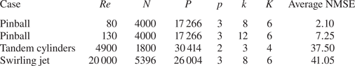
To investigate further the decoder performance, a comparison using as input low-dimensional coordinates resulting from Isomap and POD has been carried out. The NMSE of the Isomap decoder is calculated using the same  $70\,\%$ training dataset. The reconstruction NMSE with POD modes is calculated as the reconstruction error employing the first two or three modes, depending on the true dimensionality
  $p$ of the dataset. Results are summarized in figure 9 and show a clear superiority of the
  $K$NN decoder in all the cases except for the tandem cylinders. In this case, the performance of the two methods is similar, due to the rather small size of the input experimental dataset and to the sparsity of the manifold leading to large errors for isolated points, as expectable from figure 7(b).

Figure 9. Reconstruction Error of Isomap versus POD: blue, Isomap; red, POD.
This argument is further confirmed by performing a parametric study reducing the size of the dataset for the pinball test case at  $Re=80$. Reducing the dataset size to the 1/2, 1/4 and 1/8 of the original data set size leads to an increasing NMSE equal to 10 %, 15 % and 43 %.
5. Conclusions
In this paper we have developed an encoder–decoder framework based on manifold learning techniques to tackle the problem of understanding shear flows. The proposed manifold learner is Isomap and it is coupled with a  $K$NN-based decoder. We show that flows which can be described with a limited set of coherent structures are suitable candidates for manifold learning. In the applications proposed in this manuscript we have chosen phenomena whose snapshots correctly sampled all the events defining the system ‘clock’, i.e. jet and wake flows in which the measurement domain samples the evolution of the main vortical features. We have shown that Isomap correctly identifies the true dimensionality of a given dataset and that the manifolds unravelled using the Isomap encoder are representative of meaningful physical quantities and are suitable for a reduced-order modelling of shear flows. The pure physics-uninformed results in the fluidic pinball case also have a correlation with physical properties like vortex-shedding phases or the force coefficients and open ground to use this technique to model wake flows and design flow-control systems.
We have shown that when handling experimental cases with complex behaviour, despite the presence of acceptable measurement noise, the new encoder–decoder tool outperforms the classical dimensionality-reduction techniques like POD in terms of clarity and interpretability of the identified manifolds, and it is less sensitive to experimental noise. In such cases, not only the identified manifolds are more reliable, but they also distil some physical information that POD is not able to catch, including the coexistence of the two shedding regimes and transition between them in the case of the wake of two tandem cylinders.
Finally, the developed decoder proved to have outstanding capabilities in reconstructing the original flow fields from the identified manifold, allowing for the instantaneous identification of the flow state with applications to closed-loop flow control.
The proposed manifold learner may significantly reduce the dimension of the state space as compared with POD expansions with similar representation error, particularly for transient flows. Hence, the autoencoder methodology may be used for full-state estimation and control design. For both tasks, every unnecessary coordinate acts as a noise amplifier and constitutes a danger for the system to get ‘off track’. The authors actively pursue this direction.
Funding
This work has been supported by the Madrid Government (Comunidad de Madrid) under the Multiannual Agreement with Universidad Carlos III de Madrid in the line of ‘Fostering Young Doctors Research’ (PITUFLOW-CM-UC3M), and in the context of the V PRICIT (Regional Programme of Research and Technological Innovation). This work has also been partially supported by the project ARTURO, ref. PID2019-109717RBI00/AEI/10.13039/501100011033, funded by the Spanish State Research Agency. B.R.N. and N.D. acknowledge funding by the National Science Foundation of China (NSFC) through grants 12172109 and 12172111 and 12202121, by the Guandgong province, China, via the Natural Science and Engineering grant 2022A1515011492, by the Shenzhen Research Foundation for Basic Research, China, via grant JCYJ20220531095605012, and HangHua company (Dalian, China) for their scientific support. The authors warmly thank Dr F. Lückoff and Dr M. Raiola for providing the swirling jet and the tandem cylinder data sets. Funding for APC: Universidad Carlos III de Madrid (Read and Publish Carlos III University of Madrid).
Data availability statement
The data that support the findings of this study are available from the corresponding author upon reasonable request.
Declaration of interests
The authors report no conflict of interest.
Appendix A. Selection of the number of neighbours $k$ in Isomap

As discussed in § 2, selecting a proper number of neighbours  $k$ to construct the neighbouring graph
  $\boldsymbol{\mathsf{G}}$ in Isomap is a crucial decision. The unknown geodesic distances between every pair of observations in the high-dimensional manifold are approximated by the shortest paths distances between the corresponding nodes in the graph
  $\boldsymbol{\mathsf{G}}$, which depends on
  $k.$ On the one hand, a too small
  $k$ may cause a splitting of the manifold into disjoint ones and thus losing its real structure. On the other hand, if
  $k$ is too large then points which are far according to the real geodesic distance may become close by using its approximation by their shortest path in
  $\boldsymbol{\mathsf{G}}$ due to an undue number of connections (edges) and/or the existence of holes in the manifold. This phenomenon is known as short circuiting.
Different approaches have been proposed in the literature to cope with the selection of  $k$ in Isomap. In this work, we follow the methodology presented by Samko, Marshall & Rosin (Reference Samko, Marshall and Rosin2006) to determine a valid range of values
  $[k_{min},k_{max}]$ to perform the search. The lower bound of the interval,
  $k_{min},$ is selected as the smallest
  $k$ so that the neighbouring graph
  $\boldsymbol{\mathsf{G}}$ is connected. Regarding the upper bound,
  $k_{max}$, the largest value of
  $k$ is picked so that the following equation holds:
 \begin{equation} \displaystyle\frac{2E}{N} \leqslant k + 2, \end{equation}
where  $E$ is the number of edges and
  $N$ is the number of nodes in
  $\boldsymbol{\mathsf{G}}$. Once the valid range of
  $k$ is found, Samko et al. (Reference Samko, Marshall and Rosin2006) propose to pick
  $k\in [k_{min},k_{max}]$ so that the residual variance is minimum.
In all our studies in § 4 using any value in the valid range selected this way results in a low residual variance. We refer the reader to figure 10 for an illustration of the impact of the choice of  $k$ on the residual variance for the pinball dataset for
  $Re = 130$.

Figure 10. Residual variance of Isomap embedding to three-dimensional space versus different Isomap  $k$, for pinball dataset
  $Re = 130$ with the valid range of Isomap's
  $k$ according to Samko et al. (Reference Samko, Marshall and Rosin2006).
Appendix B. Different approaches to define the residual variance
There exist numerous approaches to assess the fits provided by different dimensionality reduction techniques. Regarding Isomap, the so-called residual variance as stated in (2.2) is the common choice.
Regarding POD, the classical definition of residual to assess its performance is given by
 \begin{equation} 1 - \displaystyle\frac{\displaystyle\sum_{j = 1}^p \text{var} (\boldsymbol{a}_j)}{\displaystyle\sum_{j = 1}^P \text{var} (\boldsymbol{a}_j)}, \end{equation}
where ‘var’ stands for the variance and  $\boldsymbol {a}_j$ are the mode amplitudes,
  $j=1,\ldots,P.$
The ways of measuring the fits in Isomap and POD given by (2.2) and (B1) are not comparable. In order to evaluate Isomap and POD up to the same standard, Tenenbaum et al. (Reference Tenenbaum, de Silva and Langford2000) proposed to replace the geodesic distances approximated by  $\boldsymbol{\mathsf{D}}_{\boldsymbol{\mathsf{G}}}$ in (2.2) by the pairwise Euclidean distances in the input high-dimensional space,
  $\boldsymbol{\mathsf{D}}_{\boldsymbol{\mathsf{X}}}$, where the element in row
  $i$ and column
  $j$ in
  $\boldsymbol{\mathsf{D}}_{\boldsymbol{\mathsf{X}}}$ is
  $\Vert \boldsymbol {x}_i - \boldsymbol {x}_j \Vert _2,$
  $i,j=1,\ldots,n.$ Then a related definition of residual variance for POD is
 \begin{equation} 1 - R^2(\text{vec}(\boldsymbol{\mathsf{D}}_{\boldsymbol{\mathsf{X}}}), \text{vec}(\boldsymbol{\mathsf{D}}_{\boldsymbol{\mathsf{Z}}})), \end{equation}
where  $\boldsymbol{\mathsf{D}}_{\boldsymbol{\mathsf{Z}}}$ is the matrix of Euclidean distances considering the retained principal components and
  $R^2$ refers to the squared correlation coefficient.
Nevertheless, the definition of residual variance in (B2) does not capture the ability of POD of reproducing the geodesic distances in the high-dimensional space. To do so, a different but related proposal to measure the residual variance for POD combines (2.2) and (B2) as
 \begin{equation} 1 - R^2(\text{vec}(\boldsymbol{\mathsf{D}}_{\boldsymbol{\mathsf{G}}}), \text{vec}(\boldsymbol{\mathsf{D}}_{\boldsymbol{\mathsf{Z}}})). \end{equation}
Finally, we point out that the residual variance as defined in (2.2), (B2) and (B3) may not decrease strictly when the number of dimensions increases. In other words, the correlation between a distance matrix obtained from a set of points in  $\mathbb {R}^d$,
  $\boldsymbol{\mathsf{D}}_{d}$, and another distance matrix,
  $\boldsymbol{\mathsf{D}}$, does not necessarily decrease if the distance between the embedded points in
  $\mathbb {R}^{d-1}$ by dropping one of the dimensions,
  $\boldsymbol{\mathsf{D}}_{d-1}$, is considered instead.
Figure 11 shows the values for the different definitions of residual variances presented in this work in each of the case studies in § 4 for different numbers of dimensions. The black line corresponds to (2.2), the red one is (B1), the blue is (B2) and the green is (B3). For all the dimensions considered, the residual variance of Isomap surpasses POD using definitions (2.2) and (B2).


 Open access