


1. Introduction
Binary droplet collisions are frequently encountered in natural and industrial processes, for example, droplets colliding in the air or in internal combustion engines (Faeth Reference Faeth1977). In the last three decades, binary droplet collision dynamics has been investigated experimentally (Jiang, Umemura & Law Reference Jiang, Umemura and Law1992; Qian & Law Reference Qian and Law1997; Bach, Koch & Gopinath Reference Bach, Koch and Gopinath2004; Huang, Pan & Josserand Reference Huang, Pan and Josserand2019; Pan et al. Reference Pan, Huang, Hsieh and Lu2019), numerically (Pan et al. Reference Pan, Huang, Hsieh and Lu2019; Chaitanya, Sahu & Biswas Reference Chaitanya, Sahu and Biswas2021) and theoretically (Al-Dirawi et al. Reference Al-Dirawi, Al-Ghaithi, Sykes, Castrejon-Pita and Bayly2021). Particularly, the investigation of outcome regimes is emphasised owing to their practical significance. The binary droplet collision is controlled by the competition of inertial, capillary and viscous forces, the off-centre distance (χ) between two droplet centres, and gas environments. Therefore, Weber number  $(We = \rho {D_0}V_0^2/\gamma )$, representing the ratio of inertial to capillary forces, Ohnesorge number (Oh = μ/(ρD 0γ)1/2), standing for the ratio of viscous to inertial-capillary forces, and the normalised off-centre distance (B = χ/D 0) are used to describe the collision dynamics, where ρ is the density of the liquid, D 0 is the initial diameter of droplets, γ is the surface tension, μ is the viscosity of the liquid and V 0 is the impact velocity of droplets, i.e. half of the relative velocity between droplets. However, the construction of a three-dimensional phase diagram is extremely complex, so a We–B phase diagram is frequently drawn to present outcome regimes in a certain gas environment, taking Oh as a parametric variable.
As shown in figure 1, the pioneering study on outcome regimes by Qian & Law (Reference Qian and Law1997) and the current literature (Pan, Chou & Tseng Reference Pan, Chou and Tseng2009; Pan et al. Reference Pan, Huang, Hsieh and Lu2019) reported a total of six outcomes, including coalescence (CO), bouncing (BO), reflexive separation (RES), stretching separation (SS), rotational separation (ROS) and shattering (SH). In a low-We range, Regimes CO and BO are present. Two droplets in Regime CO contact each other and merge into a larger one, whereas those in Regime BO do not touch each other but instead bounce off the compressed gas cushion between them. The separation regimes (RES, SS and ROS) take place in a high-We range but in different B ranges. Regime RES occurs in a low-B range and represents that a merged droplet after significant spreading can be transformed back into two individual droplets moving away from each other; however, Regime SS takes place in a high-B range, which is indicative of significant stretching between the two droplets and then fast separation. Regime ROS, recently proposed by Pan et al. (Reference Pan, Huang, Hsieh and Lu2019), is similar to Regime SS but in a lower B range. In addition, the merged droplet in Regime ROS has significant rotation instead of fast separation in Regime SS. When We is extremely large, Regime SH appears, and the merged droplet breaks into many small daughter droplets.

Figure 1. (a) A phase diagram of binary droplet collisions (Oh = 0.0044 and D 0 = 0.6 mm) in an atmospheric environment (Pan et al. Reference Pan, Huang, Hsieh and Lu2019). (b) Schematics of outcomes, including coalescence (CO), bouncing (BO), reflexive separation (RES), stretching separation (SS), rotational separation (ROS) and shattering (SH). The Weber numbers in the original figure of Pan et al. (Reference Pan, Huang, Hsieh and Lu2019) are four times the Weber numbers in panel (a) because the relative velocity, 2V 0, between two droplets is used by Pan et al. (Reference Pan, Huang, Hsieh and Lu2019) for calculating Weber numbers, whereas the velocity, V 0, of one droplet is considered in this work.
When comparing We–B phase diagrams with different Oh and gas environments, several intriguing phenomena are found. First, with decreasing gas pressure (p), the gas cushion becomes difficult to form so that two droplets prefer to be in direct contact with each other, and the region of Regime BO is reduced (Qian & Law Reference Qian and Law1997). Second, increasing Oh impedes Regimes ROS and RES; therefore, the boundaries between these separation regimes and coalescence regime shift towards higher Weber numbers in We–B phase diagrams (Sommerfeld & Kuschel Reference Sommerfeld and Kuschel2016; Pan et al. Reference Pan, Huang, Hsieh and Lu2019). This is attributed to the fact that a strong viscous effect can lead to remarkable viscous dissipation, impeding the transition from coalescence to these separations. Third, the boundary between Regimes CO and SS also shows the same feature in most Oh ranges; however, intriguingly, in a special Oh range (0.02 < Oh < 0.14), this boundary collapses into a single curve, showing an inertial boundary (Al-Dirawi et al. Reference Al-Dirawi, Al-Ghaithi, Sykes, Castrejon-Pita and Bayly2021). Moreover, in this Oh range, the maximum stretching factor (lmax) in Regime CO is not sensitive to Oh as well, indicating inertial behaviours (Al-Dirawi et al. Reference Al-Dirawi, Al-Ghaithi, Sykes, Castrejon-Pita and Bayly2021). Because of the inertial boundary and the inertial behaviours, the inertial regime (viscous force is ignorable compared with inertial and capillary forces) can be defined in this special Oh range from 0.02 to 0.14. Once Oh falls below or increases above this range, the boundary between Regimes CO and SS and behaviours in Regime CO become viscosity dependent, and they transition from the inertial regime to the cross-over regime (viscous force is no longer negligible).
Compared with collisions in the inertial regime (0.02 < Oh < 0.14), collisions in the cross-over regime (Oh > 0.14) are also practically required. In internal combustion engines, reducing droplet diameters can significantly enhance combustion efficiency. As the diameter of an alkane (hexadecane) droplet reduces to O(μm), its Ohnesorge number can be increased to approximately 0.26, showing that the collision of such droplets falls into the cross-over regime. Unfortunately, despite the progress in the inertial regime (0.02< Oh <0.14), the viscosity-dependent dynamics of collisions in the cross-over regime (Oh > 0.14) has not been explored in detail. Owing to the enhanced viscous effect in such a high-Oh range, Regimes RES and ROS are significantly impeded, while Regime SS remains (Sommerfeld & Kuschel Reference Sommerfeld and Kuschel2016). Identifying the boundary between Regimes CO and SS becomes important for understanding outcome regimes. Nonetheless, since the separation dynamics is no longer inertial, the viscous dissipation mechanism is altered, rendering describing the boundary extremely challenging.
For understanding the viscous dissipation mechanism, modelling the maximum spreading factor (βmax) is in demand, where βmax is the same as lmax at B = 0. Previous studies frequently model βmax by establishing an energy conservation equation from the initial state to the maximum spreading state to describe the viscous dissipation mechanism during spreading. Because the droplet is spherical at the initial state with a velocity of V 0 and forms a cylinder-like shape at the maximum spreading state with no remaining kinetic energy, the kinetic and surface energy at these states can be easily calculated. However, the calculation of the viscous dissipation during spreading is an extremely challenging task because information on evolving shapes and flow fields within the spreading droplet is additionally required. Early studies note that viscous dissipation concentrates in a cylinder-like sub-region, located at the centre of merged droplets, with stagnation flow inside it, whereas viscous dissipation is negligible near spreading rims (Jiang et al. Reference Jiang, Umemura and Law1992; Qian & Law Reference Qian and Law1997). On the basis of this point, Pan et al. (Reference Pan, Chou and Tseng2009) assumed that the stagnation flow region has a diameter of D 0/2 and a thickness of hmin, and the internal velocity gradients can be calculated by V 0/(hmin/2), where hmin represents the minimal thickness, i.e. the thickness of the merged droplet at the maximum spreading state. Their βmax model includes both We and Re (or Oh = We 1/2/Re), indicating that the model is applicable to the cross-over regime. This model only qualitatively catches the dependence of βmax on both We and Oh; however, it shows significant deviation from their experiment data at a larger Oh. In contrast, Wildeman et al. (Reference Wildeman, Visser, Sun and Lohse2016) claimed that instead of concentrating in the centre part of merged droplets, velocity gradients principally occur near the entrance of spreading rims, yielding an intriguing energy conversion feature where the stable proportion of the initial kinetic energy converts to viscous dissipation during spreading. This viscous dissipation mechanism implies that all binary droplet collisions are viscosity-independent and hence fall into the inertial regime. Recent experiment studies (Planchette et al. Reference Planchette, Hinterbichler, Liu, Bothe and Brenn2017; Al-Dirawi et al. Reference Al-Dirawi, Al-Ghaithi, Sykes, Castrejon-Pita and Bayly2021) proved that the constant proportion of viscous dissipation occurs only in a special Oh range from 0.02 to 0.14, but the proportion increases with Oh when Oh exceeds 0.14, indicating the transition from the inertial regime to the cross-over regime. Nonetheless, the viscous dissipation in the cross-over regime was not theoretically estimated by them. Therefore, the viscous dissipation mechanism needs to be satisfactorily revealed in the cross-over regime.
Nanodroplet-based technologies are rising recently, such as nanoscale inkjet printing (Galliker et al. Reference Galliker, Schneider, Eghlidi, Kress, Sandoghdar and Poulikakos2012), the preparation of high-entropy materials (Glasscott et al. Reference Glasscott, Pendergast, Goines, Bishop, Hoang, Renault and Dick2019) and so forth. Especially in inkjet printing processes, the minimal diameter of droplets is already reduced to 60 nm with an extremely high impact velocity of 250 m s−1, as reported by Galliker et al. (Reference Galliker, Schneider, Eghlidi, Kress, Sandoghdar and Poulikakos2012), which shows practical requirements for studying the dynamics of nanodroplets. Due to the occurrence of the scale effect, viscous force is enhanced at the nanoscale (Li, Zhang & Chen Reference Li, Zhang and Chen2015; Li, Li & Chen Reference Li, Li and Chen2017; Wang et al. Reference Wang, Wang, Gao, Yang, Wang and Chen2020a,Reference Wang, Wang, Xie, Liu, Wang, Yang, Gao and Wangb; Xie et al. Reference Xie, Lv, Yang and Wang2020; Wang et al. Reference Wang, Wang, Yang, Wang and Chen2021a,Reference Wang, Wang, Wang, Zhang and Chenb; Lv et al. Reference Lv, Xie, Yang, Lee, Wang and Duan2022; Wang et al. Reference Wang, Wang, He, Zhang, Yang, Wang and Lee2022a,Reference Wang, Wang, He, Zhang, Yang, Wang and Leeb). Even for the typical low-viscosity liquid, water, the Ohnesorge number of a 10 nm water nanodroplet can be larger than 0.14, implying that the collision of nanodroplets possibly falls into the cross-over regime. Recently, there have been studies on the binary nanodroplet collision, including outcome regimes and modelling βmax. Yin et al. (Reference Yin, Su, Zhang, Zhang, Xu, Hu, Zhang, Huang and Liu2021) investigated collisions of nanodroplets in a vacuum and found that Regimes BO, RES and ROS do not take place at the nanoscale in the tested We range from 0 to 300; as a result, Regimes CO, SS and SH occupy most regions of the phase diagram at the nanoscale. The strongly suppressed Regimes RES and ROS at the nanoscale accord with the macroscale feature in the cross-over regime and hence confirm the speculation that the binary nanodroplet collision falls into the cross-over regime. Zhang & Luo (Reference Zhang and Luo2019) focused on head-on binary nanodroplet collisions in a wide range of pressures from 0 to 800 kPa and found a significant difference between macroscale and nanoscale droplets. At the macroscale, increasing p can enlarge the area of Regime BO in a phase diagram and even cause bouncing for head-on collisions. For instance, the bouncing for the head-on collision of binary tetradecane droplets can take place at p = 100 kPa (Qian & Law Reference Qian and Law1997). However, at the nanoscale, bouncing is not able to take place for head-on collisions unless the gas pressure is increased to 270 kPa (Zhang & Luo Reference Zhang and Luo2019). Subsequently, Zhang & Luo (Reference Zhang and Luo2019) reported a new outcome regime at the nanoscale, i.e. a hole regime, which prefers to take place in a high-We range for head-on collisions. In addition, they established a model of βmax for head-on collisions in a vacuum, which shows relatively good agreement with their MD data in a low-We range; however, the model is found not to be able to describe βmax in a high-p range because βmax is significantly reduced with increasing p at the nanoscale. Furthermore, Zhang et al. (Reference Zhang, Zhao, Luo and Shi2021) compared collisions of nanodroplets with diameters of 10, 50 and 100 nm, and reported that the hole regime takes place for 10 and 50 nm nanodroplets but vanishes for 100 nm nanodroplets. Instead of the hole regime, Regime RES is observed for 100 nm nanodroplets, indicating the scale-dependent hole regime.
Despite preliminary identification of outcome regimes, neither the regime boundaries nor the viscous dissipation mechanism during spreading is satisfactorily described at the nanoscale. Due to the naturally high Oh of nanodroplets, binary nanodroplet collisions principally fall into the cross-over regime, indicating further difficulty in solving these two issues. It should be emphasised that even at the macroscale, such key issues are not well revealed in the cross-over regime. As a result, investigating the regime boundaries and the viscous dissipation mechanism at the nanoscale is expected to not only fill the gap at the nanoscale, but also contribute to the understanding of the collision dynamics at the macroscale.
This study investigates binary collisions of nanodroplets that can be naturally considered high-viscosity droplets, aiming to reveal the boundaries of outcome regimes and the viscous dissipation mechanism in the cross-over regime. First, in a vacuum, binary collisions of nanodroplets with different diameters and wide We and B ranges are tested in a systematic and thorough way to identify outcome regimes. A scaling law is subsequently derived to describe the boundary between Regimes CO and SS by considering the balance between kinetic and surface energy, with its prefactor including the ratio (α) of the viscous dissipation during spreading to the initial kinetic energy. Second, also in the vacuum condition, the maximum spreading factor is modelled by establishing an energy conservation equation, in which an assumption of velocity gradients is proposed with the help of extracted velocity distributions in nanodroplets from MD simulations. Using the model of βmax, α is obtained. Here, it needs to be emphasised that the scaling law of stretching separation boundary and the model of βmax are expected to be valid for both nanodroplets and high-viscosity macroscale droplets. Third, the collision of nanodroplets is investigated at high gas pressures. In this part, Regime BO and the effect of gas pressure on βmax are explored.
2. Simulation method
MD simulations, which are implemented by the LAMMPS (large-scale atomic/molecular massively parallel simulation) package, are used to investigate the binary droplet collision dynamics at the nanoscale. Figure 2 shows the schematic of the simulation system with a dimension of 100 × 100 × 100 nm3, where periodic boundary conditions are applied in all three directions. The two equal-sized water nanodroplets are produced by face-centred cubic (fcc) crystals based on the corresponding density at 300 K. This work attempts to reveal the collision dynamics of nanodroplets with diameters ranging from several nanometres to hundreds of nanometres. To reduce the computational cost, the nanodroplets with relatively low diameters of 6(±0.3), 8(±0.3) and 10(±0.4) nm are simulated, containing water molecule numbers of 3782, 8968 and 17 517, respectively. This treatment is valid because, throughout the nanoscale, nanodroplets should follow the same collision dynamics, provided that the dominant dimensionless number group (We, Oh and B) is the same. Here, the calculations of the dimensionless numbers (We and Oh) use the average values of the diameters (i.e. 6, 8 and 10 nm), and these three diameters create a range of Oh from 0.35 to 0.45.

Figure 2. Schematic of the simulation system containing two nanodroplets, where two views for observing the dynamic behaviour of nanodroplets are shown.
MD simulations solve Newton's equations of motion to get the evolution of all particles in the simulation system, including the information of position, ri = (xi, yi, zi), and velocity, Vi = (Vx ,i, Vy ,i, Vz ,i), i.e.
 \begin{equation}{m_i}\frac{{{\textrm{d}^2}{\boldsymbol{r}_i}}}{{\textrm{d}{t^2}}} = {m_i}\frac{{\textrm{d}{\boldsymbol{V}_i}}}{{\textrm{d}t}} = {\boldsymbol{F}_i} = \sum\limits_{j {\ne} i} - {\boldsymbol{\nabla }U({r_{ij}})} ,\end{equation}
where mi is the mass of particle i, Fi is the force exerted on particle i by others, U(rij) is the potential function to describe the interaction between particles i and j, and rij is the distance between them.
Many water models have been developed to describe water within the framework of the MD simulation method. Owing to different assumptions of water structure and potential, the water described by these models has different physical properties from each other. Moreover, almost all current water models for MD simulations can only partially reproduce the key properties (ρ, γ and μ) (Molinero & Moore Reference Molinero and Moore2009). Therefore, the liquid described by each water model can be treated as an artificial liquid. However, fortunately, for the binary collision dynamics of equal-sized droplets at the nanoscale, when the values of the dimensionless parameter group (We, Oh and B) remain constant, the collision dynamics is uniquely determined, regardless of the choice of liquids. In other words, in MD simulations, the investigation of the collision dynamics is independent of the choice of potentials (see supplementary figure S1 available at https://doi.org/10.1017/jfm.2023.1069). Based on this point, the mW water model is chosen to describe the water because it is a coarse-grained model that can significantly reduce the computational cost. This water model is expressed as
 \begin{gather}{U_{mW}}({r_{ij}}) = \sum\limits_i {\sum\limits_{j > i} {{\varphi _1}({r_{ij}})} } + \sum\limits_i {\sum\limits_{j {\ne} i} {\sum\limits_{k > j} {{\varphi _2}({r_{ij}},{r_{ik}},{\theta _{ijk}})} } } ,\end{gather}
 \begin{gather}{\varphi _1}({r_{ij}}) = A\varepsilon \left[ {B{{\left( {\frac{\sigma }{{{r_{ij}}}}} \right)}^p} - {{\left( {\frac{\sigma }{{{r_{ij}}}}} \right)}^q}} \right]\,\textrm{exp}\left( {\frac{\sigma }{{{r_{ij}} - a\sigma }}} \right),\end{gather}
 \begin{gather}{\varphi _2}({r_{ij}},{r_{ik}},{\theta _{ijk}}) = {\lambda _\textrm{t}}\varepsilon {[\textrm{cos}\,{\theta _{ijk}} - \textrm{cos}\,{\theta ^0}]^2}\,\textrm{exp}\left( {\frac{{\gamma \sigma }}{{{r_{ij}} - a\sigma }}} \right)\,\textrm{exp}\left( {\frac{{\gamma \sigma }}{{{r_{ik}} - a\sigma }}} \right),\end{gather}
where A = 7.049556277, B = 0.6022245584, p = 4, q = 0, γ = 1.2, a = 1.8 and θ 0 = 109.47° are from the original Stillinger–Weber potential (Stillinger & Weber Reference Stillinger and Weber1985), whereas the tetrahedral parameter λt (describing the strength of the tetrahedral interaction), the energy scale (ε) and the distance scale (σ) are tuned to λt = 23.15, ε = 0.2684 eV and σ = 0.23925 nm for producing the mW model (Molinero & Moore Reference Molinero and Moore2009). According to Molinero & Moore (Reference Molinero and Moore2009) and Jacobson, Kirby & Molinero (Reference Jacobson, Kirby and Molinero2014), the properties of mW water are ρ = 996 kg m−3, γ = 66 mN m−1 and μ = 0.2837 mPa s. It should be noted that these parameters are all calculated from MD simulations based on the mW model. For example, considering a periodic simulation box with a slab of liquid inside it, as shown in figure S2, the surface tension can be calculated by  $1/2{L_N}[\langle {\,p_N}\rangle - \langle {\,p_T}\rangle ]$ (Kirkwood & Buff Reference Kirkwood and Buff1949), where L N is the length of the simulation box in the direction normal to the slab of liquid, and
  $\langle {\,p_N}\rangle$ and
  $\langle {\,p_T}\rangle$ are the time-averaged components of the pressure tensors tangential (pT) and normal (pN) to the slab of liquid over an equilibrium simulation. It is worth noting that the choice of the mW model may lead to a problem of reproducing the saturated vapour pressure of water. The mW model is proposed by Molinero & Moore (Reference Molinero and Moore2009) to describe the molecular interaction of water, by modifying the original Stillinger–Weber potential that is used to model the solid and liquid forms of silicon (Stillinger & Weber Reference Stillinger and Weber1985). Silicon has an extremely low saturated vapour pressure; for example, its saturated vapour pressure is not larger than 15 Pa at a super-high temperature of 2102 K according to Stevanovic (Reference Stevanovic1984); therefore, the mW water model significantly underestimated the saturated vapour pressure of water so that the gas space can be approximately treated as a vacuum at 300 K, as shown in figure S3(a–c). However, such an underestimation is proven not to affect the reliability of the mW water model for the prediction of nanodroplet collision dynamics (please see supplementary material, figure S3). In addition, as shown in figure S4, the change in the numbers of gas molecules during collisions are extracted for mW water, TIP3P water and LJ argon at Oh = 0.49 and We = 25, whose βmax have been proven the same (figure S1), indicating that MD simulations can capture the evaporation during collisions and such evaporation does not affect the collision dynamics.
At the macroscale, the choice of gas has been proven to affect the collision process due to the different gas molecular weight and viscosity; however, Regime BO can always take place once the gas pressure is large enough, no matter the kind of gas (Qian & Law Reference Qian and Law1997). In this work, the most focused issue in a gas environment is whether Regime BO can still exist at the nanoscale instead of detailed effect on collision dynamics, so only the gas pressure is concerned. Because argon (Ar) with a simple structure can result in high computational efficiency and is gaseous at 300 K, it is chosen to fill the simulation box for creating gas pressures. The interactions of Ar-water and Ar–Ar are both described by the 12-6 Lennard-Jones potential, expressed as
 \begin{equation}{U_{LJ}}({r_{ij}}) = 4\varepsilon \left[ {{{\left( {\frac{\sigma }{{{r_{ij}}}}} \right)}^{12}} - {{\left( {\frac{\sigma }{{{r_{ij}}}}} \right)}^6}} \right],\quad {r_{ij}} < {r_{cut}},\end{equation}
where rcut is the cut-off distance. The parameters for Ar–water and Ar–Ar interactions are ε Ar-water = 0.0085 eV, σ Ar-water = 3.286 Å, ε Ar–Ar = 0.0103 eV, and σ Ar–Ar = 3.405 Å, respectively, where the parameters for Ar–Ar interactions are from Yaguchi, Yano & Fujikawa (Reference Yaguchi, Yano and Fujikawa2010). For these interactions, r cut is long enough to be set to 1 nm, as shown in figure S5. To test the effect of ambient gas at high pressures, the droplets are set far away from each other before collisions and the simulation system is filled with Ar atoms to create gas pressures of 120 and 450 kPa.
Each simulation includes three processes with a time step of 2 fs. The first process is an equilibrium process, conducted in the NVT ensemble (canonical ensemble) with a constant temperature of 300 K by the Nose–Hoover thermostat. In this process, two nanodroplets are fixed at a certain distance away from each other. After the simulation is implemented for 2 ns, the system achieves thermodynamic equilibrium and the equilibrium process ends. The second process is an approach process running in the NVE ensemble (micro-canonical ensemble), in which the two nanodroplets move close to each other with a given velocity. Once the two nanodroplets start to touch each other, the second process ends. The third process is a collision process (i.e. an outcome process), and many outcomes are possibly observed, depending on the collision condition, such as coalescence, separation and so forth. According to our tests, the formation of outcomes (i.e. the maximum stretching length does not change for coalescence, separation takes place for stretching separation and generated daughter droplets retract to spheres for shattering) are mostly within 500 ps; therefore, the collision process for all cases is implemented for 1 ns that is long enough to observe the whole collision process. The calculations for the cases of 6, 8 and 10 nm nanodroplets without additional gas molecules will require approximately 5, 10 and 16 h, respectively, on four threads on Intel Xeon E5-2697 v4 processors. The position and velocity of each water molecule are recorded every 1 ps for further analysis. For ensuring reliable statistics, we repeated the simulations of collisions of two 10 nm nanodroplets at low, medium and high Weber numbers (i.e. We = 6, 24 and 74) five times and recorded βmax, as shown in Table S1. The maximum relative deviation from the mean value of βmax at each Weber number does not exceed 1.5 %, showing the reliable statistics of the simulations.
3. Results and discussion
3.1. Outcome regimes of collisions in a vacuum
3.1.1. Effects of We and B
In this section, the outcome regimes of binary droplet collisions in a vacuum are discussed. At the macroscale, a total of six outcomes are reported, as shown in figure 1. However, there are only three outcomes for binary nanodroplet collisions, including CO, SS and SH, as shown in figure 3. As expected, due to the vacuum condition and the high-Oh effect, Regimes BO, RES and ROS are not found in the tested We range from 1 to 110 at the nanoscale. Here, instead of considering the formation of holes as a final outcome as done by the previous studies (Zhang & Luo Reference Zhang and Luo2019), the formation of holes is regarded as an intermediate outcome in this work, i.e. each final outcome can be further divided into two branches by whether holes form during collisions. As a result, the final outcomes with holes are further marked by an additional red circle, as shown in figure 3. For example, the outcome of coalescence with holes is marked by a blue square (representing coalescence) with an additional red circle (standing for a hole). Each outcome will be discussed in detail with the help of its typical snapshots, as shown in figures 4 and 5. The discussion of the outcome regimes is divided into two groups: (i) a low-B range (B < 0.2) and (ii) a high-B range (B ≥ 0.2).

Figure 3. Phase diagram of binary nanodroplet collisions with Oh = 0.35, including coalescence (CO), stretching separation (SS) and shattering (SH). It should be emphasised that the hole is an intermediate outcome marked by a red circle based on the final outcomes (CO, SS and SH).

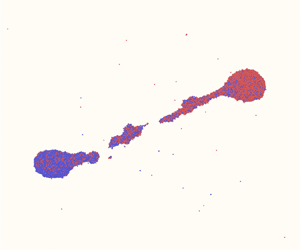
Figure 4. Snapshots of head-on binary nanodroplet collisions at We = (a) 24, (b) 54, (c) 74 and (d) 109. The numbers shown in panel (d) at t = 30 and 40 ps highlight the positions of jetted fingers. It is worth noting that when the thickness of the peripheric rim is larger than the one at the centre of liquid films, only the outline of the rim can be seen in the front view. To show the relative thickness between the rim and the centre of liquid films, supplemented sliced snapshots near the beginning of forming holes for panel (c,d) are shown in figure S6(e,f).

Figure 5. Snapshots of off-centre binary nanodroplet collisions at We = (a) 24, (b) 54, (c) 74 and (d) 109.
(i) Low-B range (B < 0.2)
In the low-B range, a binary nanodroplet collision is more like a head-on collision. Figure 3 shows that as We increases, nanodroplets sequentially undergo Regimes CO and SH, with holes forming in a high-We range. At a relatively low Weber number of 24, the collision is in Regime CO, as shown in figure 4(a). The two nanodroplets first merge into a single droplet and spread to the maximum spreading diameter without residual kinetic energy (t = 35 ps); subsequently, by releasing the surface energy stored in the deformation at the maximum spreading state, the merged droplet retracts (t = 75 ps) and reflexively stretches to the maximum extent against the collision direction (t = 120 ps). The reflexive separation does not take place, and the merged droplet eventually equilibrates into a sphere under the action of surface tension (t = 200 ps). At the macroscale, at a low Weber number of 8 (Qian & Law Reference Qian and Law1997), the merged droplet can stretch and form a dumbbell-like shape, i.e. the critical shape to generate Regime RES. However, at the nanoscale, although the Weber number is increased to a larger value of 54, the dumbbell-like shape is still not observed, as shown in figure 4(b). Eventually, no reflexive separation is found in all the present simulation cases, as shown in figure 3. This may be ascribed to the fact that the enhanced viscous force significantly increases the viscous dissipation during spreading. As We continues to increase to 74, the two droplets still coalesce into a merged droplet (t = 10 ps), but holes are generated in the retraction process (t = 60 ps), as shown in figure 4(c). Subsequently, the holes are refilled at t = 140 ps, and the following dynamic behaviours of the merged nanodroplet are identical to those in Regime CO without holes.
Here, it should be noted that no holes can be observed during binary droplet collisions at the macroscale (Pan et al. Reference Pan, Chou and Tseng2009; Liu & Bothe Reference Liu and Bothe2016). Using MD simulations, Zhang et al. (Reference Zhang, Zhao, Luo and Shi2021) have also found that the hole outcome will no longer be observed as the diameter of droplets increases to 100 nm. Therefore, the generation of holes for binary droplet collisions is limited to small scales. At the nanoscale, the outcome of holes is reported not only in head-on collisions (Zhang & Luo Reference Zhang and Luo2019; Zhang et al. Reference Zhang, Zhao, Luo and Shi2021) but also in another similar process, i.e. the impact of a nanodroplet on a smooth solid surface (Li et al. Reference Li, Li and Chen2017; Wang et al. Reference Wang, Wang, Wang, Zhang and Chen2021b). Li et al. (Reference Li, Li and Chen2017) and Wang et al. (Reference Wang, Wang, Wang, Zhang and Chen2021b) interpreted that holes at the nanoscale are induced by the violent vibration of liquid films at relatively high Weber numbers. However, this interpretation is possibly doubtful because the centre of the liquid film is expected to experience the most violent vibration, but holes disorderly form in the interior of the film instead of at the centre, as shown in figure 4(c) and snapshots in the previous studies (Li et al. Reference Li, Li and Chen2017; Wang et al. Reference Wang, Wang, Wang, Zhang and Chen2021b).
Another possible mechanism, thermal fluctuations, is proposed here to interpret the generation of holes. Moseler & Landman (Reference Moseler and Landman2000) investigated liquid jets at the nanoscale using MD simulations and claimed that the instability is induced by thermal fluctuations. To prove this, they added a stochastic stress tensor to the standard NS equations, and a stochastic lubrication equation (SLE) was derived to simulate the liquid jets at the nanoscale. Good agreement between the MD and SLE results is found. Subsequently, Hennequin et al. (Reference Hennequin, Aarts, van der Wiel, Wegdam, Eggers, Lekkerkerker and Bonn2006) experimentally attested that thermal fluctuations can play an important role in liquid instability at very small scales and proved that the extended NS equations are able to describe the instability of liquid when thermal fluctuations are dominant. Based on these studies, it can be concluded that thermal fluctuations are important for liquid instability at the nanoscale, and MD simulations can accurately simulate the effect of thermal fluctuations. Recently, Zhang, Sprittles & Lockerby (Reference Zhang, Sprittles and Lockerby2019) investigated the instability of liquid films with thicknesses of 1.18, 1.57 and 1.96 nm. Their MD results show that the films have unstable surfaces and spontaneously break up at their internal parts due to the action of thermal fluctuations. Based on this result, as expected, the liquid film at the maximum spreading state in figure 4(c), which has a thickness of less than 2 nm, does have unstable surfaces due to thermal fluctuations. As a result, the thermal fluctuations and the strong vibration at relatively large Weber numbers jointly induce the formation of holes. This insight not only interprets why holes disorderly form in the interior part of liquid films, but also answers why no holes generate when the diameter of nanodroplets increases to 100 nm (Zhang et al. Reference Zhang, Zhao, Luo and Shi2021).
After the formation of holes, hole-refilling is observed, as shown in figure 4(c). Here, its mechanism is discussed, with the help of a series of detailed snapshots. As shown in figure S6(a), holes are formed in the retraction stage at 50 ps. With the action of surface tension, the holes rapidly expand and merge into a large one from 50 to 69 ps. Meanwhile, the outer rim has started to retract at considerable speed. At t = 69 ps, the merged hole stops expanding because it comes up against the retracting rim. After that, the merged hole begins to retract along with the retracting rim from 69 to 83 ps, and eventually, the hole is completely refilled at t = 85 ps. Therefore, the hole-refilling can be attributed to the intensely retracting rim. In addition, the hole-refilling process is also observed by other potential models (an LJ liquid argon, the TIP3P water and the SPCE water), as shown in figure S6(b–d). As a result, the hole-refilling does not rely on the choice of potential models and hence is physical.
At an extremely large We of 109, the collision enters Regime SH. Figure 4(d) shows that the merged droplet has an irregular and unstable periphery during spreading (t = 10 and 17 ps) with holes appearing and growing in its internal part (t = 36 and 40 ps). Instead of the formed rim when holes emerge at We = 74, as shown in figure S6(e), such an irregular and unstable periphery at We = 109 inhibits the formation of retracting rim, as shown in figure S6(f); as a result, the expending of holes cannot be stopped and eventually the merged droplet shatters (t = 70 ps). Pan et al. (Reference Pan, Chou and Tseng2009) who studied macroscale binary droplet collisions in Regime SH have pointed out that the irregular and unstable periphery is attributed to Rayleigh–Taylor instability. The difference in the unstable periphery between the macroscale and the nanoscale lies in that the formed fingers at the macroscale are lathy, but those at the nanoscale are stubby. In addition, Wang et al. (Reference Wang, Wang, Wang, Zhang and Chen2021b) also reported that the splash of a nanodroplet impacting a solid surface is due to Rayleigh–Taylor instability. According to these studies, the shattering in binary nanodroplet collisions is expected to be caused by the Rayleigh–Taylor instability as well. Inspired by Wang et al. (Reference Wang, Wang, Wang, Zhang and Chen2021b), the Rayleigh–Taylor instability during the fast spreading of thin films is tested by comparing the MD results of the interfacial waves at the periphery of nanodroplets with the theoretical results of the Rayleigh–Taylor instability. According to the Rayleigh–Taylor instability theory developed by Allen (Reference Allen1975), the finger number can be calculated by N = [kρ/(12γ)]1/2D 0βmax, where k is the deceleration rate calculated by  $V_0^2/{D_0}$. Using βmax ≈ 3 extracted from the snapshots at 30 and 40 ps in figure 4(d), N is theoretically obtained as 9, which shows good agreement with the MD result at 30 and 40 ps in figure 4(d), and therefore indicates that the present data are consistent with the Rayleigh–Taylor instability theory. Further tests for nanodroplets with diameters of 6 and 8 nm are also implemented to prove this consistency, as shown in figure S7.
(ii) High-B range (B ≥ 0.2)
In the high-B range, the off-centre effect becomes significant. As shown in figure 5(a), at a low We of 24, the higher B reduces the head-on area between the two droplets and enhances the stretching behaviour (t = 15 ps). Subsequently, the merged droplet is continuously stretched by the residual initial kinetic energy, with the central liquid bridge becoming thinner (t = 80 ps), accompanied by rotational motion. After the centre of the droplet reaches the thinnest thickness (t = 220 ps), the liquid bridge gradually grows (t = 340 ps) until its thickness increases to the ends’ thickness of the merged droplet (t = 400 ps), showing Regime CO. When We increases to 54, larger off-centre kinetic energy is present, leading to the transition from Regime CO to SS. As shown in figure 5(b), the early collision process in Regime SS, including the stretching (t = 15 ps) and the formation of a thin liquid bridge (t = 50 ps), does not show a significant difference from the one in Regime CO shown in figure 5(a), whereas in the later process, the liquid bridge does not stop becoming further thinner (t = 120 ps) and finally breaks up (t = 150 ps), generating separated daughter droplets (t = 180 ps). At a larger We of 74, holes generate at the centre of the merged droplet during stretching, as shown in figure 5(c). Furthermore, the deformation of merged droplets is enhanced and the number of holes is raised with a further increase in We, as shown in figure 5(d).
3.1.2. Modelling the boundary of the stretching separation regime
Regimes CO and SS occupy most regions of the phase diagram at the nanoscale, as shown in figure 3, and thereby, identifying the boundary between them is important for understanding the outcome regimes. In an early study, Jiang et al. (Reference Jiang, Umemura and Law1992) assumed the separation process as two short cylinders grazing and finally departing from each other and correspondingly established a model for describing the boundary, expressed as B = c 1We −1/2[1 + c 2 $\mu$γ −3/2ρ 1/2
 $D^{1/2}_{0}$], where c 1 and c 2 are both fitting parameters. The model can satisfactorily fit the boundary in wide collision conditions, whereas these fitting parameters vary with the properties of liquid, indicating a lack of universality. This may arise from the fact that the actual shape of stretching droplets greatly deviates from the excessively constrained assumption of the cylinder shape. More recently, Al-Dirawi et al. (Reference Al-Dirawi, Al-Ghaithi, Sykes, Castrejon-Pita and Bayly2021) experimentally found that the stretching separation of merged droplets follows a universal critical maximum stretching factor (lmax ,cr) of 3.35, above which the stretching separation can take place. They, therefore, established a model of lmax to predict the boundary. Here, lmax is considered to be contributed by head-on and off-centre parts when B > 0.2, expressed as lmax = βmax + s(B − 0.2), where s is an off-centre fitting function as s = 0.049We + 2.58. The model of βmax is built based on the assumption of the constant proportion (α) of the viscous dissipation during spreading to the initial kinetic energy at each Oh, and s is obtained by data fitting as a We-dependent function. Substituting lmax ,cr = 3.35 in the model of lmax, the equation of the stretching separation boundary is obtained. This model can accurately predict the boundary between Regimes CO and SS in both inertial and cross-over regimes. In the inertial regime, the boundary is independent of Oh, so the model with a constant value of α = 0.65 can predict the boundary at different Oh; in the cross-over regime, because the boundary is dependent on Oh, the model can hold only when adjusting the value of α corresponding to Oh. However, the quantitative relationship between Oh and α has not been established. Furthermore, using the model of lmax to predict the boundary is complex because it requires the calculation of βmax from an implicit expression even if α is known. To simplify this, a simple scaling law of the stretching separation boundary is directly established in this work, in which α is incorporated into the prefactor of it. This scaling law is expected to be valid both in the inertial regime by a constant α and in the cross-over regime by an Oh-dependent α. Despite using Oh-dependent α in the cross-over regime, α is not extracted from experiments or simulations but is obtained by a model of βmax in which the viscous dissipation during spreading is directly calculated.
The scaling law of the stretching separation boundary is derived in this section. During off-centre collision, the off-centre kinetic energy, expressed as  ${\sim} {P_o}\rho D_0^3V_0^2$, principally contributes to the stretching of the merged droplet, where P o = −0.5B 3 + 1.5B is the off-centre factor (for detailed information, please see Appendix A). During stretching, the off-centre kinetic energy converts to viscous dissipation and surface energy stored in the deformation. Once the residual off-centre kinetic energy after overcoming viscous dissipation exceeds the surface energy required for triggering the stretching separation, the stretching separation could take place. Since B does not affect the viscous dissipation proportion during stretching (Al-Dirawi et al. Reference Al-Dirawi, Al-Ghaithi, Sykes, Castrejon-Pita and Bayly2021), the residual off-centre kinetic energy can be expressed as
  ${\sim} (1 - \alpha ){P_o}\rho D_0^3V_0^2$. The required surface energy is difficult to directly express, but it should satisfy the following two restrictions. One is that it must increase when B decreases, which corresponds to the fact that reducing the off-centre effect can hinder the stretching separation behaviour. The other is that it must be infinite when B = 0, because stretching separation is impossible to take place in head-on collision processes, indicating that B must be larger than 0. These restrictions yield a simple scaling assumption for the required surface energy as
  ${\sim} \gamma D_0^2/B$. As a result, the scaling law for describing the stretching separation boundary is obtained as
  $\gamma D_0^2/B\sim (1 - \alpha ){P_o}\rho D_0^3V_0^2$. After rearranging this scaling law, the boundary equation of the transition from Regime CO to SS is
 \begin{equation}We = C{( - 0.5{B^4} + 1.5{B^2})^{ - 1}},\end{equation}
where C is the prefactor of the scaling law. This scaling law shows the energy balance between the off-centre kinetic energy and the required surface energy, with the viscous dissipation during stretching to be incorporated into its prefactor as C ~ (1 − α)−1. When the viscous dissipation becomes larger (i.e. α and C are both larger), a smaller ratio of the initial kinetic energy can be used to promote the stretching for separation, leading to an increase in the requirement for the initial kinetic energy and also to the shifting of the critical Weber number towards high values. Using C = 4.8, (3.1) well fits the boundary between Regimes CO and SS, as shown in figure 3.
It should be emphasised that in the inertial regime, C is a constant due to constant α; however, in the cross-over regime, a large Oh increases viscous dissipation and hence leads to an increased C. To validate whether this scaling law covers the stretching separation boundary in both the inertial and cross-over regimes, another two phase diagrams for mW nanodroplets with Oh = 0.39 (D 0 = 8 nm) and 0.45 (D 0 = 6 nm) from this work are shown in figure 6(a,b), and an additional phase diagram for TIP4P nanodroplets with Oh = 0.58 from Yin et al. (Reference Yin, Su, Zhang, Zhang, Xu, Hu, Zhang, Huang and Liu2021) is shown in figure S8. Moreover, the experimental data on the stretching separation boundaries from the previous studies (Sommerfeld & Kuschel Reference Sommerfeld and Kuschel2016; Sommerfeld & Pasternak Reference Sommerfeld and Pasternak2019; Al-Dirawi et al. Reference Al-Dirawi, Al-Ghaithi, Sykes, Castrejon-Pita and Bayly2021) are also used to test the scaling law, as shown in figure 6(c,d). This scaling law can satisfactorily match the stretching separation boundaries at both the nanoscale and the macroscale. In a relatively low-Oh range, C is almost constant; however, in a relatively large-Oh range, C increases with Oh. To exhibit the relationship between C and Oh, the data of C versus Oh are drawn in figure 6(e). This figure shows that C remains constant at 3.8 in the inertial regime but increases with Oh in the cross-over regime. Nonetheless, it should be indicated that all values of C in figure 6(a–d) are obtained by regression. As a result, the model of βmax will be established in the next section to obtain α and hence C by C ~ (1 − α)−1.

Figure 6. (a,b) Phase diagrams of binary nanodroplet collisions with Oh = (a) 0.39 and (b) 0.45, where the solid line represents the proposed scaling law. (c,d) Boundary data of the stretching separation regime from (c) Al-Dirawi et al. (Reference Al-Dirawi, Al-Ghaithi, Sykes, Castrejon-Pita and Bayly2021) and Sommerfeld & Pasternak (Reference Sommerfeld and Pasternak2019), and (d) Sommerfeld & Kuschel (Reference Sommerfeld and Kuschel2016). (e) Values of prefactor (C) obtained from figures 3, 6(a–d) and figure S8 at various Oh, where the values of C regressed from figures 3 and 6(a,b) are marked by black squares, and the value regressed from figure S8 is marked by a green square. Here, the dashed line represents a constant value of 3.8, and the solid line represents the predicted value by the scaling law of C ~ (1 − α)−1, where the prefactor of this scaling is adopted as 1, and α is obtained by the model of βmax, i.e. (3.20).
3.2. Modelling βmax in a vacuum
In this section, the head-on collision is discussed by modelling its feature parameter βmax for understanding the viscous dissipation mechanism and obtaining the ratio (α) of the viscous dissipation during spreading to the initial kinetic energy. The energy conservation equation of spreading is frequently established by considering kinetic energy (Ek), surface energy (Es) and viscous dissipation (Edis) from the initial state to the maximum spreading state, expressed as
 \begin{equation}{E_{k,0}} + {E_{s,0}} = {E_{s,m}} + {E_{dis}},\end{equation}
where subscripts 0 and m denote the initial state and the maximum spreading state, respectively. Since the net flux of molecules across the symmetry plane can be safely regarded as null, the head-on binary droplet collision can be considered as a droplet impacting an imaginary symmetry plane. Therefore, only one of the two droplets is chosen as the subject in modelling, as shown in figure 7(a). This treatment brings convenience to the discussion of binary droplet collisions and the impacts of droplets on solid surfaces later.

Figure 7. (a) Schematics of a head-on collision process and a symmetry plane, where, due to the symmetry, the collision can be considered as a nanodroplet impacting the imaginary symmetry plane, bringing the convenience of modelling βmax. (b–d) Velocity contours of head-on binary nanodroplet collisions at We = 85 at t = (a) 8, (b) 13 and (c) 18 ps. The left side shows the velocity component in the impact direction, Vz, whereas the right side represents the velocity component in the spreading direction, Vr.
The spherical shape of a nanodroplet before collision yields the expressions of Ek ,0 and Es ,0 as
 \begin{gather}{E_{k,0}} = {\textstyle{1 \over {12}}}{\rm \pi} \rho D_0^3V_0^2,\end{gather}
 \begin{gather}{E_{s,0}} = \gamma {\rm \pi}D_0^2.\end{gather}
According to Li et al. (Reference Li, Li and Chen2017), Es ,m for the nanodroplet at the maximum spreading state can be expressed as
 \begin{equation}{E_{s,m}} = {\rm \pi}D_0^2\gamma \left( {\frac{1}{3}\beta_{max}^2 + \frac{2}{3}\frac{1}{{{\beta_{max}}}}} \right)\!.\end{equation}
In a recent study (Al-Dirawi et al. Reference Al-Dirawi, Al-Ghaithi, Sykes, Castrejon-Pita and Bayly2021), it has been proven that α is constant in the inertial regime but increases with Oh in the cross-over regime. However, the quantitative relationship between α and Oh has not been satisfactorily established in the cross-over regime. Herein, the viscous dissipation is estimated by integration of the dissipation function, ϕ, as follows:
 \begin{gather}{E_{dis}} = \int_0^{{t_s}} {\int_\varOmega {\phi \,\textrm{d}\varOmega \,\textrm{d}t} } ,\end{gather}
 \begin{gather}\phi = \mu \left( {\frac{{\partial {v_i}}}{{\partial {x_j}}} + \frac{{\partial {v_j}}}{{\partial {x_i}}}} \right)\frac{{\partial {v_i}}}{{\partial {x_j}}}.\end{gather}
Considering Vθ = 0, (3.7) is simplified as
 \begin{equation}\phi = 2\mu \left[ {{{\left( {\frac{{\partial {V_r}}}{{\partial r}}} \right)}^2} + {{\left( {\frac{{{V_r}}}{r}} \right)}^2} + {{\left( {\frac{{\partial {V_z}}}{{\partial z}}} \right)}^2} + \frac{1}{2}{{\left( {\frac{{\partial {V_r}}}{{\partial z}} + \frac{{\partial {V_z}}}{{\partial r}}} \right)}^2}} \right],\end{equation}
where Ω is the volume of droplets, ts is the spreading time, i.e. the time span for one of the two droplets from just touching the symmetry plane to attaining the maximum spreading state, Vr is the velocity component in the spreading direction (radial direction), Vz is the velocity component in the impact direction (axial direction), r is the coordinate of the spreading direction (radial direction) and z is the coordinate of the impact direction (axial direction). According to (3.8), the estimation of viscous dissipation requires information on velocity gradients; however, the velocity distribution feature within the nanodroplet in head-on collisions is still unknown. Zhang & Luo (Reference Zhang and Luo2019) assumed that the velocity gradient of ∂Vr/∂z dominates the viscous dissipation during spreading, expressed as ∂Vr/∂z = (rV 0)/(RH), where R is the spreading radius and H is the height of droplets. Unfortunately, the model of βmax from Zhang & Luo (Reference Zhang and Luo2019) based on this velocity assumption does not accurately fit MD data in a high-We range. This may be attributed to the fact that the no-slip condition usually takes place when liquid flows on a solid surface but significantly diverges from the free-spreading film in such head-on collisions. For precisely understanding velocity distributions within droplets, velocity contours are extracted from MD simulations by the following method. The simulation box is divided into many units with a dimension of 0.5 × 0.5 × 0.5 nm3, and then the velocity components in spreading and impact directions in each unit are calculated by
 \begin{equation}\left.
{\begin{array}{*{20}{@{}c@{}}} {{V_r}\textrm{ =
}\dfrac{{\displaystyle\sum_{i = 1}^n {{V_{r,i}}}
}}{n},}\\ {{V_z}\textrm{ =
}\dfrac{{\displaystyle\sum_{i = 1}^n {{V_{z,i}}}
}}{n},} \end{array}}
\right\}\end{equation}
\begin{equation}\left.
{\begin{array}{*{20}{@{}c@{}}} {{V_r}\textrm{ =
}\dfrac{{\displaystyle\sum_{i = 1}^n {{V_{r,i}}}
}}{n},}\\ {{V_z}\textrm{ =
}\dfrac{{\displaystyle\sum_{i = 1}^n {{V_{z,i}}}
}}{n},} \end{array}}
\right\}\end{equation}where n is the number of molecules in a unit, and i is the ith molecule. The velocity contours of the merged nanodroplet during head-on collision at We = 85 are shown in figure 7(b–d). Each velocity component (Vr or Vz) shows a linear profile in its own direction (spreading or impact direction) but does not change in the other direction. In other words, ∂Vr/∂r (or ∂Vz/∂z) is constant, but ∂Vr/∂z (or ∂Vz/∂r) can be neglected. As a result, the velocity gradients of ∂Vr/∂r and ∂Vz/∂z play dominant roles in the viscous dissipation during spreading. Because of Vr |r = 0 = 0 and Vr |r = R = Vs, the distribution of Vr within nanodroplets can be expressed as
 \begin{equation}{V_r} = \frac{r}{R}{V_s},\end{equation}
where Vs is the spreading velocity at the edge of the spreading film. According to the continuity equation,
 \begin{equation}\frac{{\partial {V_r}}}{{\partial r}} + \frac{{\partial {V_z}}}{{\partial z}} + \frac{{{V_r}}}{r} = 0,\end{equation}
the expression of Vz can be derived as
 \begin{equation}{V_z} =- \frac{{2z}}{R}{V_s}.\end{equation}
Unlike the assumption of velocity gradients, ∂Vr/∂z = (rV 0)/(RH), satisfying the no-slip condition (i.e. the shear flow feature), (3.10) and (3.12), following the free-slip condition (i.e. the extensional flow feature), can match better with the velocity contours shown in figure 7(b–d). Combining (3.8) with (3.10) and (3.12), the dissipation function is obtained,
 \begin{equation}\phi = \mu \frac{{12}}{{{R^2}}}V_s^2.\end{equation}
By integration with respect to space, (3.6) is transformed to
 \begin{equation}{E_{dis}} = \int_0^{{t_s}} {[12{\rm \pi} H\mu V_s^2]\,\textrm{d}t} .\end{equation}
According to the volume conservation,  ${\rm \pi} D_0^3/6 = {\rm \pi}D{(t)^2}H$, H could be replaced by β(t), expressed as
 \begin{equation}H = \frac{2}{3}\frac{{{D_0}}}{{{\beta ^2}(t)}}.\end{equation}
Substituting (3.15) in (3.14) yields
 \begin{equation}{E_{dis}} = \int_0^{{t_s}} {\left[ {8{\rm \pi} \mu {D_0}V_s^2 \cdot \frac{1}{{{\beta^2}(t)}}} \right]\textrm{d}t} .\end{equation}
In addition, the differential of time, dt, can be replaced by the differential of the spreading factor, dβ(t), expressed as
 \begin{equation}\textrm{d}\beta (t) = \frac{{\textrm{d}D(t)}}{{{D_0}}} = 2\frac{{\textrm{d}R(t)}}{{{D_0}}} = \frac{{2{V_s}\,\textrm{d}t}}{{{D_0}}}.\end{equation}
Rearranging (3.17) leads to
 \begin{equation}\textrm{d}t = \frac{{{D_0}\,\textrm{d}\beta (t)}}{{2{V_s}}}.\end{equation}
Substituting (3.18) in (3.16), the expression of the viscous dissipation during spreading is finally obtained as
 \begin{equation}{E_{dis}} = 4{\rm \pi} \mu D_0^2{V_s}\left( {1 - \frac{1}{{{\beta_{max}}}}} \right)\!.\end{equation}
Combining (3.2) with (3.3)–(3.5) and (3.19) leads to
 \begin{equation}\frac{1}{3}\beta _{max}^2 + \frac{2}{3}\frac{1}{{{\beta _{max}}}} - 1 = \frac{{We}}{{12}} - 4{C_{vf}}W{e^{1/2}}Oh\left( {1 - \frac{1}{{{\beta_{max}}}}} \right),\end{equation}
where the velocity factor is Cvf = Vs/V 0. During spreading, the spreading velocity varies nonlinearly from a high value at the initial state to zero at the maximum spreading state. Here, an equivalent constant spreading velocity is adopted by data fitting. The spreading velocity (Vs) stems from the collision of droplets with the impact velocity (V 0), and therefore, it should increase with V 0. In addition, the internal extensional flow feature has been incorporated into this model, which relates the velocities in the impact and spreading directions. Based on these clues, it is expected that the spreading velocity scales as the impact velocity (i.e. Cvf is a constant) in the cross-over regime. According to the data of βmax shown in figure 8(a), Cvf is taken as 0.48. For testing the universality of this fitting value, with Cvf = 0.48 as input, the proposed model of βmax is compared with the simulation data not only of mW water nanodroplets with diameters from 5 to 10 nm but also of TIP3P water nanodroplets with diameters of 8 and 10.9 nm (figure 8). To verify whether the molecular orientation and structure have special effects on βmax, figure 8(e) includes two series of data for both the mW water and the TIP3P water at the same Oh, where the mW water is a monatomic model and the TIP3P is a full-atom model. Good agreement is shown between the model and the MD simulation results for nanodroplets with various diameters and Weber numbers based on different water models, indicating the universality of the proposed model in the cross-over regime.

Figure 8. (a–e) Comparisons between theoretical results and MD data from both current and previous studies.
Using the proposed model of βmax, the value of Edis is calculated at various We. As shown in figure 9(a), the predicted Edis show linear dependence on Ek ,0 at each Oh, indicating a constant value of α = Edis/Ek ,0. This is consistent with the experimental observation in the previous studies (Planchette et al. Reference Planchette, Hinterbichler, Liu, Bothe and Brenn2017; Al-Dirawi et al. Reference Al-Dirawi, Al-Ghaithi, Sykes, Castrejon-Pita and Bayly2021). By fitting the slopes of Edis–Ek ,0 curves, α at different Oh is obtained. Figure 9(b) shows the data of α from previous studies (Willis & Orme Reference Willis and Orme2003; Planchette et al. Reference Planchette, Hinterbichler, Liu, Bothe and Brenn2017; Huang, Pan & Josserand Reference Huang, Pan and Josserand2019; Al-Dirawi et al. Reference Al-Dirawi, Al-Ghaithi, Sykes, Castrejon-Pita and Bayly2021) in both the inertial and cross-over regimes. In the cross-over regime, the ratios (α) from Willis & Orme (Reference Willis and Orme2003) are lower than those from Huang, Pan & Josserand (Reference Huang, Pan and Josserand2019) and Al-Dirawi et al. (Reference Al-Dirawi, Al-Ghaithi, Sykes, Castrejon-Pita and Bayly2021). To the best of our knowledge, such differences have not been satisfactorily interpreted before. Two possible reasons are proposed here, i.e. the non-Newtonian effect and the gas pressure effect. However, Al-Dirawi et al. (Reference Al-Dirawi, Al-Ghaithi, Sykes, Castrejon-Pita and Bayly2021) reported that HPMC and glycerol aqueous solutions show Newtonian behaviours in their study; in addition, the silicone oils used by Willis & Orme (Reference Willis and Orme2003) and Huang, Pan & Josserand (Reference Huang, Pan and Josserand2019) can also safely be considered as Newtonian fluids, according to the study of Vázquez-Quesada et al. (Reference Vázquez-Quesada, Mahmud, Dai, Ellero and Tanner2017). As a result, the non-Newtonian effect is excluded. Because the experiments of Willis & Orme (Reference Willis and Orme2003) were conducted in a vacuum, whereas those of the other studies were in an atmosphere, the lower α from Willis & Orme (Reference Willis and Orme2003) is more possibly ascribed to the gas pressure effect. As expected, the proposed model of βmax, which is based on binary nanodroplet collisions in a vacuum, underpredicts the macroscale data of α in the atmosphere but shows good agreement with the macroscale data in the vacuum (Willis & Orme (Reference Willis and Orme2003)). Using α obtained by the model of βmax in the cross-over regime, the prefactor, C ~ (1 − α)−1, of (3.1) is also determined, which shows good agreement with the data in the cross-over regime, as shown in figure 6(e). It should be emphasised that the value of C regressed from the phase diagram of Yin et al. (Reference Yin, Su, Zhang, Zhang, Xu, Hu, Zhang, Huang and Liu2021), who simulated the collisions by two TIP4P water nanodroplets, is also satisfactorily predicted by C ~ (1 − α)−1, indicating that the collision dynamics obtained by different potential models of liquids is the same when the value of the dimensionless number group remains constant. This further proves that it is safe to investigate binary nanodroplet collisions by such a coarse-grained mW water model.

Figure 9. (a) Results of Edis varying with Ek ,0 at different Oh calculated by (3.20) and the corresponding linear fitting results. (b) Comparison between the predicted α by (3.20) and the measured α in previous experimental studies, where the dashed line presents a constant value of α in the inertial regime and the solid line shows the predicted α with the method shown in panel (a).
Although the established model of βmax successfully covers the viscous dissipation mechanism in the cross-over regime, the transition from the inertial to the cross-over regime has not been properly interpreted. Here, a possible reason for the transition is discussed based on the flow features in the inertial (Wildeman et al. Reference Wildeman, Visser, Sun and Lohse2016) and cross-over (this work) regimes. In the inertial regime, Wildeman et al. (Reference Wildeman, Visser, Sun and Lohse2016) reported a viscosity-independent ratio of the viscous dissipation during spreading to the initial kinetic energy for head-on binary droplet collisions. They interpreted that this specific viscous dissipation mechanism corresponds to the flow feature that velocity gradients principally concentrate in the entrance region of the rim. However, as shown in figure 7(b–d), when collisions are in the cross-over regime, the velocity gradients are violent in entire droplets instead of only in the entrance region of the rim. Therefore, the transition mechanism from the inertial to the cross-over regime may result from the violent viscous dissipation extending from the entrance region of the rim to the entire droplet.
Since the impact of droplets on solid surfaces is similar to head-on binary droplet collisions, the current model of βmax in the cross-over regime is expected to be valid for impacting nanodroplets on solid surfaces as well. It is also desired to provide insights into the viscous dissipation mechanism during spreading on solid surfaces at the nanoscale because there is still a debate on the flow feature of nanoscale impact dynamics. Li et al. (Reference Li, Zhang and Chen2015) reported that the velocity gradient of ∂Vz/∂z = V 0/H dominates the viscous dissipation, whereas Li et al. (Reference Li, Li and Chen2017) claimed that ∂Vr/∂z = (rV 0)/(RH) contributes to the viscous dissipation. Nonetheless, both of them ignored some important velocity gradients. Wang et al. (Reference Wang, Wang, Gao, Yang, Wang and Chen2020a) proposed another velocity distribution for calculating the viscous dissipation, i.e. Vr = Vsrz/(RH) and Vz = −z 2Vs/(RH), based on which no velocity gradient is ignored. These expressions satisfy the no-slip condition. However, the no-slip condition is significantly violated for impacting nanodroplets on solid surfaces (Koplik, Banavar & Willemsen Reference Koplik, Banavar and Willemsen1988), implying that these expressions do not hold for the nanoscale impact on solid surfaces, and also showing the similarity between the impact on solid surfaces and head-on binary droplet collision at the nanoscale. Therefore, it is expected that the proposed model can also predict βmax for the impact of nanodroplets on solid surfaces. Nonetheless, the model can fit the data on a surface with θ = 180° only when the fitting parameter (Cvf) is modified to 0.85, as shown in figure 10(a). This may be attributed to the fact that solid surfaces render the viscous dissipation of impacting nanodroplets on them larger than that of binary droplet collisions. Wang et al. (Reference Wang, Wang, Yang, Wang and Chen2021a) reported that when θ > 73°, the wettability has a relatively weak effect on the maximum spreading factor (βmax) for the impact of nanodroplets on solid surfaces. Therefore, the data of βmax on surfaces with θ from 73° to 148° are also used to further test the proposed model here. It is found that although the proposed model does not include the effect of contact angles, it still shows good agreement when θ ≥ 125°, as shown in figure 10(b), with a mean relative error of 2.1 %. When θ < 125°, the accuracy of the proposed model is reduced with underestimation in a low-We range and overestimation in a high-We range, as shown in figure 10(c). This can be attributed to the following two reasons. First, in a low-We range, stronger wettability can spontaneously increase βmax. Therefore, in the low-We range, the proposed model slightly underestimates the value of βmax. Second, stronger wettability may also reduce the slip effect, leading to increased viscous dissipation. This viscous dissipation is more significant at high We. Consequently, the proposed model overestimates βmax at high Weber numbers. The combination of these two reasons results in a steeper dependency of βmax on We than MD data when θ < 125°. However, even if wettability comes into play, the prediction accuracy of our model remains acceptable, with the mean relative error only increasing to 6.4 %. To further demonstrate that the prediction accuracy is indeed improved by modifying the estimation of viscous dissipation in the proposed model, a recently developed nanoscale no-slip βmax model is also considered for comparison (Li et al. Reference Li, Li and Chen2017). Comparing this no-slip model with the MD data reveals that the estimation of viscous dissipation has a dominant effect on both prediction accuracy and the dependence of βmax on We, as shown in figure 10(b,c). Therefore, our proposed model, using slip-based viscous dissipation estimation, not only improves prediction accuracy but also further elucidates the viscous dissipation mechanism behind nanoscale droplet impact on solid surfaces. In addition to the comparison with MD data, to further ensure the established model is useful in physical reality, the only data point on the maximum spreading factor of nanodroplets in a real inkjet printing process from Galliker et al. (Reference Galliker, Schneider, Eghlidi, Kress, Sandoghdar and Poulikakos2012) is also taken into consideration. As shown in figure 10(b), without any further modification, the established model can well fit the experimental value, proving the practical significance of the established model.

Figure 10. (a) Comparison among the MD data for impacting nanodroplets on solid surfaces with θ = 180°, the scaling law of βmax ~ We 1/2 with a prefactor of 0.26 and the proposed model with Cvf = 0.85. (b,c) Comparison between the proposed model with Cvf = 0.85 and the MD data of βmax for nanodroplets on solid surfaces with (b) θ ≥ 125° and (c) θ < 125°. In addition, an experimental data point is also considered for comparison in panel (b).
It should be emphasised that, intriguingly, in the wide We range from approximately 30 to 110, the data of βmax for nanodroplets coincide with the scaling law of βmax ~ We 1/2, as shown in figure 10(a); however, βmax ~ We 1/2 has never been observed in any experiments for millimetre-sized droplets impacting solid surfaces (Josserand & Thoroddsen Reference Josserand and Thoroddsen2016). Here, the agreement between the prediction result of (3.20) and the scaling law of βmax ~ We 1/2 at the nanoscale indicates that the possible condition for the occurrence of the scaling of βmax ~ We 1/2 is the extensional flow feature. If that is not the case, the spreading droplet will have the shear flow feature, and the velocity gradient of ∂Vr/∂z( = (rV 0)/(RH)) for the shear flow will make the expression of viscous dissipation include a term of  $\beta _{max}^5$ (Li et al. Reference Li, Li and Chen2017; Wang et al. Reference Wang, Wang, Gao, Yang, Wang and Chen2020a), leading to remarkable viscous dissipation with increasing βmax and hence making the scaling law of βmax ~ We 1/2 impossible. This argument provides a possible reason why βmax ~ We 1/2 has never been observed for millimetre-sized impacting droplets on solid surfaces (Josserand & Thoroddsen Reference Josserand and Thoroddsen2016).
3.3. Effect of ambient gas
All discussion in §§ 3.1 and 3.2 is implemented in a vacuum condition by mW droplets, therefore under the dimensionless parameter group of We, Oh and B. However, the effect of ambient gas is also an important parameter affecting the collision dynamics of droplets. In previous macroscale studies (Jiang et al. Reference Jiang, Umemura and Law1992; Qian & Law Reference Qian and Law1997), to incorporate the influence of ambient gases, the ambient pressure p is usually included to describe the collision dynamics. Nonetheless, because p is not a dimensionless number, a variety of gas types is also frequently considered to fully understand the effect of ambient gases. On outcomes, the previous study (Qian & Law Reference Qian and Law1997) has shown that ambient gas mainly affects Regime BO, while its effect on other regimes (CO, SS and RES) is relatively weak. Specifically, in a wide range of ambient gas pressures, the boundaries between Regimes CO, SS and RES only alter slightly, while the boundaries between Regime BO and other outcomes can change dramatically. For βmax, Jiang et al. (Reference Jiang, Umemura and Law1992) have pointed out that the work on ambient gas by droplets is negligible compared with the viscous dissipation inside the droplets, so it is believed that the ambient gas does not affect βmax. Another piece of evidence is that the head-on transition between Regimes CO and RES, which is strongly dependent on the viscous dissipation during head-on collisions, does not change significantly over a wide pressure range of 100 to 800 kPa (Qian & Law Reference Qian and Law1997). Therefore, the effect of ambient gas at the macroscale can be summarised. For outcomes, the ambient gas mainly affects the boundaries between Regime BO and other regimes, depending on both the type and pressure of the gas. For βmax, the effect of ambient gas is not significant. At the nanoscale, the effect of ambient gas on collision dynamics is also important to explore. Here, the discussion of ambient gas below is divided into two groups based on gas pressures, i.e. low ambient gas pressure and high ambient gas pressure.
3.3.1. Low gas pressure
In this work, four different liquid models, including SPCE, TIP3P, mW and LJ (for argon), have been used to create different saturated vapour environments. Among the three water models (SPCE, TIP3P and mW), TIP3P can satisfactorily reproduce the saturated vapour pressure of water in experiments (3.5 kPa at no curvature), while mW significantly underestimates the saturated vapour pressure (close to a vacuum). The saturated vapour pressure of SPCE is intermediate between that of TIP3P and mW. The LJ model creates a saturated vapour pressure of up to 79 kPa for argon (at no curvature) (Yaguchi et al. Reference Yaguchi, Yano and Fujikawa2010). In addition to these scenarios, a system containing mW water droplets, filled with argon gas, is also considered to produce a vapour pressure that is the same as the saturated vapour pressure of water in experiments. In summary, a range of gas pressures from approximately 0 (mW) to 79 kPa (Ar) and different types of gases (mW water vapour, SPCE water vapour, TIP3P water vapour, and argon vapour and gas) are tested in the low ambient pressure range. Here, the pressure range is characterised by vapour pressures at no curvature, but to avoid ambiguity, it is worth noting that the Kelvin effect can occur according to the diameters of droplets. Controlling Oh and B of these droplets and comparing their βmax over a wide range of Weber numbers, it is found that when the values of the dimensionless numbers (We, Oh, B) are the same, they have almost the same values of βmax, independent of the ambient gas type and ambient gas pressure, as shown in figure S1. Therefore, for collisions at low ambient gas pressures (p < 79 kPa), it can be believed that the collision dynamics is still governed by the dimensionless numbers (We, Oh, B). This is also consistent with the results of macroscale studies. Therefore, the conclusions from §§ 3.1 and 3.2 are equally applicable to the collision dynamics at low gas pressures.
3.3.2. High gas pressure
When exposed to high ambient gas pressures, nanodroplets appear to show different dynamics from that of macroscale droplets. For macroscale collisions, Qian & Law (Reference Qian and Law1997) have reported that with increasing p, the area of Regime BO in phase diagrams increases, and the other regimes can be significantly suppressed. This is because the correspondingly increasing density of the gas cushion entrapped between two approaching droplets hinders them from merging. However, the extremely small scale of nanodroplets renders the stable gas cushion difficult to form, so the gas between them is more likely to be squeezed out, making the bouncing almost impossible. A recent study (Zhang, Jiang & Luo Reference Zhang, Jiang and Luo2016) indicated that bouncing can still take place for nanodroplets if the gas pressure is increased to 270 kPa. However, from the bouncing snapshots reported by them, the nanodroplets stop approaching due to the existence of a gas cushion. After that, the two nanodroplets are suspended in gas environments. In traditional bouncing, when two droplets approach each other, the gas cushion between droplets is compressed with high pressure, resulting in the flattening of the droplets and hence the energy conversion from kinetic energy to surface energy; subsequently, when the initial kinetic energy is exhausted, the stored surface energy is released to induce the bouncing of droplets away from each other. Therefore, the bouncing reported by Zhang et al. (Reference Zhang, Jiang and Luo2016) is different from traditional bouncing. Within this context, whether traditional bouncing can take place at the nanoscale should be further verified.
In addition to Regime BO, the viscous dissipation during head-on collisions is also concerned at the nanoscale. The macroscale study (Jiang et al. Reference Jiang, Umemura and Law1992) indicated that the work by droplets on gas can be negligible compared with the viscous dissipation inside the droplets. However, Zhang & Luo (Reference Zhang and Luo2019) reported that at each We, βmax significantly decreases with increasing p. Although they ascribed this to the gas cushion effect, the relationship between energy dissipation and the gas cushion effect has not been quantitatively described.
The phase diagrams at p = 120 and 450 kPa at 300 K, with ρg = 1.42 and 6.82 kg m−3, respectively, are shown in figure 11. It is found that the increased gas pressure does not significantly affect the boundary between Regimes CO and SS, and Regime BO still does not occur. For nanodroplets, the gas environment may not be a continuum. According to the kinetic theory of gases, the mean free path of gas atoms can be calculated by λ = kBT/(21/2 ${\rm \pi}$d 2p), and λ is obtained as 60.6 and 16.2 nm at p = 120 and 450 kPa, respectively, where k B is the Boltzmann constant and d = 3.58 Å is the effective diameter of argon atoms (Guggenheim & McGlashan Reference Guggenheim and Mcglashan1960). Therefore, the Knudsen numbers (Kn = λ/D 0) for these two gas environments are 6.06 at p = 120 kPa and 1.62 at 450 kPa. Such large values of Kn indicate that the gas environments are in the transitional flow regime, and importantly, strong rarefaction effects emerge (Gad-el-Hak Reference Gad-el-Hak1999). Because stretching separation frequently takes place at a relatively high value of off-centre distance, the viscous drag force for each nanodroplet can be approximately treated as that for a single nanodroplet moving in gas environments. At these large Kn of 1.62 and 6.06, the rarefaction effect has been strong, which significantly reduces viscous drag force. Therefore, it can be expected that the reduced viscous drag does not show a remarkable change when Kn decreases from 6.06 to 1.62. Accordingly, when gas pressure increases from 120 to 450 kPa, the boundary between Regimes CO and SS is almost not altered, as shown in figure 11(a,b).

Figure 11. (a,b) Phase diagrams at gas pressures of (a) 120 and (b) 450 kPa. The comparison of βmax between MD simulation results and theoretical predictions at gas pressures of (c) 120 and (d) 450 kPa.
Zarin (Reference Zarin1970) and Loth (Reference Loth2008) proposed that when the particle Reynolds number (Re p = ρgD 0V 0/ $\mu_{g}$) is lower than 45, the motion of particles (i.e. nanodroplets) is dominated by the rarefaction effect but not by the compressibility effect. For argon, ρg = 1.42 and 6.82 kg m−3 at p = 120 and 450 kPa, respectively;
  $\mu_{g}$ is not sensitive to p when p < 10 Mpa (Trappeniers et al. Reference Trappeniers, Botzen, van den Berg and van Oosten1964) and equals 22.5 μPa s (Berg & Burton Reference Berg and Burton2012). Using D 0 = 10 nm and the maximum impact velocity (V 0,max = 850 m s−1), the maximum Rep is 2.58, which is far lower than 45 and shows the dominant rarefaction effect. Owing to the large Knudsen numbers and the dominant rarefaction effect, the stable gas cushion cannot form at the nanoscale, which is responsible for no Regime BO being observed at the nanoscale.
Compared with Regime SS, both Regime SH and the hole regime are remarkably suppressed, and especially Regime SH does not occur in the tested We range. More importantly, the maximum spreading factors are also reduced when increasing gas pressures, as shown in figure 11(c,d). During head-on collisions, the gas molecules between two approaching nanodroplets will be squeezed out, leading to the viscous drag force for head-on nanodroplets being larger than that for a single nanodroplet moving in the same gas environment, and the viscous drag force will continuously increase with the distance between two nanodroplets decreasing. More importantly, the increase in viscous drag force can be strengthened by decreasing Kn (Chun & Koch Reference Chun and Koch2005). As a result, when gas pressure increases from 120 to 450 kPa (i.e. Kn decreases from 6.06 to 1.62), the reduction in the maximum spreading factor is more significant, as shown in figure 11(c,d).
In these high-pressure environments, part of the initial kinetic energy is additionally consumed due to the viscous drag force caused by the displacement of gas molecules by nanodroplets. Here, the consumed kinetic energy by the viscous drag force is added to (3.20) by an additional energy term scaling with the initial kinetic energy, i.e.  ${C_g}(\rho D_0^3V_0^2/12)$, leading to the simply modified model of βmax as
 \begin{equation}\begin{array}{l} \dfrac{1}{3}\beta _{max}^2 + \dfrac{2}{3}\dfrac{1}{{{\beta _{max}}}} - 1 = (1 - {C_g})\dfrac{{We}}{{12}} - 4{C_{vf}}W{e^{1/2}}Oh\left( {1 - \dfrac{1}{{{\beta_{max}}}}} \right),\\ \end{array}\end{equation}
where Cg is a fitting parameter. When gas pressure increases (Kn decreases), the displaced number of gas molecules increases and the viscous drag force is enhanced, so Cg should be positively related to p. Using Cg = 0.22 at p = 120 kPa and 0.27 at p = 450 kPa, the modified model can well fit the data on collisions in high gas pressure environments. This agreement indicates the effectiveness of the insight that the displacement of gas molecules by nanodroplets consumes part of the initial kinetic energy and the viscous drag force increases with decreasing Kn during head-on collisions at the nanoscale.
4. Conclusions
In this study, the binary nanodroplet collision dynamics is studied through MD simulations, aiming to reveal outcome regimes and estimate the viscous dissipation during spreading. Simulations are implemented for droplet diameters (6, 8 and 10 nm) in wide ranges of We (1–109) and B (0–0.9). In addition, the effect of gas pressures (vacuum, 120 and 450 kPa) is also discussed.
In a vacuum, outcome regime diagrams are constructed in a We–B coordinate system, where three outcomes, coalescence (CO), stretching separation (SS) and shattering (SH), are successfully identified, whereas bouncing (BO), reflexive separation (RES) and rotational separation (ROS), which have been extensively reported for macroscale collisions, are not observed. This result is explained by the fact that the reduction in droplet sizes increases Oh significantly, thereby enhancing the viscous effect. In other words, natural high-viscosity nanodroplets are responsible for the non-observed three outcomes in the tested We range in this work. In addition, holes are generated for the observed outcomes in a high-We range, and, as an intermediate outcome, their formation is attributed to the vibration-induced rupture of the nanoscale film and the action of thermal fluctuations. The splashing rims in Regime SH are ascribed to the Rayleigh–Taylor instability, which is proven by comparing the finger numbers between MD simulations and theoretical results.
Since Regimes CO and SS occupy most regions of phase diagrams, the focus is subsequently placed on the development of the boundary equation between them. The boundary equation is established based on the criterion that the residual off-centre kinetic energy after overcoming the viscous dissipation can still be larger than the surface energy required for triggering the stretching separation. As a result, the estimation of viscous dissipation becomes a determinant. The flow feature extracted from MD simulations shows that the extensional flow assumption well fits the velocity gradient distributions in both impact and spreading directions. Based on this, viscous dissipation is calculated, and the ratio (α) of the viscous dissipation during spreading to the initial kinetic energy is estimated for various We and Oh. The result shows that the ratio is independent of We and remains constant at a fixed Oh; it increases with Oh due to the enhanced viscous effect. Using the obtained Oh-dependent ratio, the boundary equation successfully predicts the boundaries between Regimes CO and SS for both nanoscale and macroscale binary droplet collisions. It is worth noting that, owing to intricate viscous dissipation mechanisms, the relationship between α and Oh is still an issue of concern in the cross-over regime for macroscale binary droplet collisions. Therefore, the estimation of viscous dissipation in this work also provides a possible insight into understanding the energy conversion of macroscale collisions when the viscous force is no longer negligible.
Another contribution of this work is that a model of the maximum spreading factor is developed for head-on binary nanodroplet collisions based on the estimation of viscous dissipation. The model shows good agreement with almost all available data on βmax. In addition, based on similarity, this model is also extended to predict the maximum spreading factor for the impact of a nanodroplet on solid surfaces. A thorough test indicates that with a constant fitting parameter of Cvf = Vs/V 0 = 0.85, the model fits MD data on solid surfaces with θ ranging from 73° to 180° satisfactorily. More importantly, this model also shows good agreement with the available experimental data on nanodroplets impacting solid surfaces in an inkjet printing process.
Finally, binary nanodroplet collisions are also examined at two gas pressures of 120 and 450 kPa. The result shows that bouncing is not triggered even if the pressure increases to 450 kPa. This unexpected result indicates that there is a different pressure effect between macroscale and nanoscale collisions. A possible cause of the absence of Regime BO is that the rarefaction effect is dominant instead of the compressibility effect. This rarefaction effect also contributes to the fact that the boundary between Regimes CO and SS is not significantly altered. However, the maximum spreading factor of merged nanodroplets is remarkably suppressed at high gas pressures because the displacement of gas molecules by nanodroplets consumes part of the initial kinetic energy. To test this insight, a kinetic energy term consumed by gas is added to the model of βmax. The modified model can satisfactorily fit MD results of βmax at different pressures (p = 120 and 450 kPa).
Supplementary material
Supplementary material is available at https://doi.org/10.1017/jfm.2023.1069.
Funding
This study was partially supported by the State Key Program of National Natural Science of China (no. 51936004) and Science Fund for Creative Research Groups of the National Natural Science Foundation of China (no. 51821004).
Declaration of interests
The authors report no conflict of interest.
Appendix A. Calculation of the off-centre factor (Po)
The off-centre factor represents the volume of one in two droplets out of the projection of the other one, as shown in figure 12. The values of Po at various B are obtained numerically, as shown in figure 13. With the help of a polynomial fitting procedure, the expression of Po is determined as
 \begin{equation}{P_o} =- 0.5{B^3} + 1.5B.\end{equation}
This expression shows good agreement with the numerical results. Since the parameter Po is controlled only by the off-centre parameter (B), the expression is universal.

Figure 12. Front and side views of binary droplet collisions, where the off-centre volume (Voo) and the total volume of one droplet (Vot) are shown schematically.

Figure 13. Numerical results of Po at various B with different numerical mesh sizes (Dm/D 0) of 0.004, 0.01 and 0.2, where Dm denotes the side length of each cubic mesh. Using polynomial fitting, the expression of Po is obtained as Po = −0.5B 3 + 1.5B.


