


1. Introduction
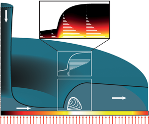
Free-surface liquid jet impingement is a practical cooling method in a wide range of technical applications. The design of jet-impingement cooling systems requires a good knowledge of the flow field on the target surface. Such a flow is schematically shown in figure 1, where the liquid spreads out from the stagnation region in a thin radial film and undergoes a sudden increase in the film height, called circular hydraulic jump (CHJ), at the jump radius,  $r_{j}$. The CHJs pose a major challenge in the analysis of jet impingement problems, because they exhibit different flow structures depending on the strength of the jump. Based on the interface curvature and the flow structure in the jump region, the following classification of CHJs can be inferred from the literature (see also figure 1):

Figure 1. Schematic illustration of a circular jet impinging vertically upon a horizontal plate subjected to a constant heat flux (CHF)  $( \dot {q} )$. Various flow structures, type 0 to type IIb, can occur depending on the strength of the jump. Finally the jump can also become unstable with air entrainment.
(i) type 0 – CHJ without any reversal flow in the jump region (Liu & Lienhard Reference Liu and Lienhard1993; Ellegaard et al. Reference Ellegaard, Hansen, Haaning and Bohr1996);
(ii) type Ia – CHJ with a single separation bubble on the wall (Ellegaard et al. Reference Ellegaard, Hansen, Haaning and Bohr1996);
(iii) type Ib – CHJ with a single roller underneath the interface (Askarizadeh et al. Reference Askarizadeh, Ahmadikia, Ehrenpreis, Kneer, Pishevar and Rohlfs2020, Reference Askarizadeh, Ehrenpreis, Kneer and Rohlfs2021);
(iv) type IIa – CHJ with a roller underneath the interface and a separation bubble directly afterwards on the wall (Liu & Lienhard Reference Liu and Lienhard1993; Ellegaard et al. Reference Ellegaard, Hansen, Haaning and Bohr1996);
(v) type IIb – double CHJ containing both a roller and a separation bubble (Liu & Lienhard Reference Liu and Lienhard1993; Bush, Aristoff & Hosoi Reference Bush, Aristoff and Hosoi2006; Askarizadeh et al. Reference Askarizadeh, Ahmadikia, Ehrenpreis, Kneer, Pishevar and Rohlfs2020);
(vi) the unstable CHJ with air entrainment (Liu & Lienhard Reference Liu and Lienhard1993; Ellegaard et al. Reference Ellegaard, Hansen, Haaning and Bohr1996).
Unfortunately, there is currently no comprehensive theory that characterises all types of CHJs and reflects the flow structure in the jump region. A typical approach in the investigation of CHJs is to reduce the Navier–Stokes equations to boundary layer equations (BLEs), since the radial thin film flow has a very small height compared with the radial dimensions. The main difference in comparison with regular BLEs is that an additional equation to determine the height of the film is required. Furthermore, this height determines the pressure term in the radial momentum equation. Such BLEs for thin film flows were numerically solved by Higuera (Reference Higuera1994) and de Vita et al. (Reference de Vita, Lagrée, Chibbaro and Popinet2020) for two-dimensional planar flows and also for radially spreading axisymmetric flows (Higuera Reference Higuera1997). The latter is of interest in this study.
A common approach to analytically describe the axisymmetric jump problem, is to find descriptions for the flow before and after the jump and to connect these by a discontinuous change of the flow variables at the jump position (Watson Reference Watson1964; Bohr, Dimon & Putkaradze Reference Bohr, Dimon and Putkaradze1993). However, such an approach is not able to reproduce the internal structure of CHJs. In this context, Bohr, Putkaradze & Watanabe (Reference Bohr, Putkaradze and Watanabe1997) introduced an averaging theory (AT) in which a third-order polynomial is assumed for the radial velocity profile over the film height, whose coefficients depend on the radius. The coefficients are determined using the boundary conditions (BCs), evaluation of the radial momentum equation on the plate and the radial momentum equation integrated over the height of the film. The chosen order of the polynomial together with the conditions for determining the coefficients lead to a non-self-similar velocity profile along the radius. The hereby achieved flexibility of the velocity profile results in a model which is able to render the flow structures ahead, in and after the jump region of the type Ia (Bohr et al. Reference Bohr, Putkaradze and Watanabe1997; Watanabe, Putkaradze & Bohr Reference Watanabe, Putkaradze and Bohr2003).
Being able to describe the flow field in the jump region, the introduced AT (Bohr et al. Reference Bohr, Putkaradze and Watanabe1997) can be used to study heat transfer in CHJs of type Ia. So far, jet impingement heat transfer has been thoroughly studied from the stagnation point (Liu, Gabour & Lienhard Reference Liu, Gabour and Lienhard1993; Rohlfs et al. Reference Rohlfs, Ehrenpreis, Haustein and Kneer2014) up to the jump position (Liu & Lienhard Reference Liu and Lienhard1989; Liu, Lienhard & Lombara Reference Liu, Lienhard and Lombara1991) and corresponding correlations for determining the heat transfer coefficient have been proposed. However, theoretical analysis of the heat transfer problem in the jump region has not yet been reported. In addition, relevant numerical (Sung, Choi & Yoo Reference Sung, Choi and Yoo1999; Askarizadeh et al. Reference Askarizadeh, Ahmadikia, Ehrenpreis, Kneer, Pishevar and Rohlfs2020) and experimental (Ishigai et al. Reference Ishigai, Nakanishi, Mizuno and Imamura1977; Stevens Reference Stevens1988) studies on heat transfer in the jump region are seldom in the literature. The complicated flow physics in the jump region, the lack of a comprehensive theory to determine the flow structure of CHJs, and a possible laminar to turbulent transition through the jump (Ishigai et al. Reference Ishigai, Nakanishi, Mizuno and Imamura1977) can be pointed out as reasons for the little available information on heat transfer in the jump region. In this regard, the AT introduced by Bohr et al. (Reference Bohr, Putkaradze and Watanabe1997) is further developed in this study to describe heat transfer in CHJs of type Ia. The extended AT, called AT for heat transfer (ATHT), is then compared with fully resolved numerical simulations (FRNSs) to show the applicability of the model to predict the temperature field in the jump region.
2. Problem statement
This section briefly presents the conservation equations describing the flow and heat transfer in radial thin film flows. The governing equations are simplified by applying boundary layer (BL) assumptions and physical constraints inherent to thin-layer film flows. This set of simplified equations together with the BCs will be used in the following section to develop a model for determining the flow and temperature fields.
2.1. Conservation equations
For an axisymmetric, incompressible, steady state thin film flow with constant fluid properties, the governing equations can be written in cylindrical coordinates as follows:
 $$\begin{gather} \frac{\partial (\tilde{r}\tilde{u})}{\partial \tilde{r}} + \frac{\partial (\tilde{r}\tilde{w})}{\partial \tilde{z}} = 0, \end{gather}$$
 $$\begin{gather}\tilde{u}\frac{\partial \tilde{u}}{\partial \tilde{r}} + \tilde{w} \frac{\partial \tilde{u}}{\partial \tilde{z}} =-\frac{1}{\rho}\frac{\partial \tilde{p}}{\partial \tilde{r}} + \nu \left( \frac{\partial^{2} \tilde{u}}{\partial \tilde{r}^{2}} + \frac{\partial}{\partial \tilde{r}} \left( \frac{\tilde{u}}{\tilde{r}} \right) + \frac{\partial^{2} \tilde{u}}{\partial \tilde{z}^{2}} \right), \end{gather}$$
 $$\begin{gather}\tilde{u}\frac{\partial \tilde{w}}{\partial \tilde{r}} + \tilde{w} \frac{\partial \tilde{w}}{\partial \tilde{z}} =-\frac{1}{\rho}\frac{\partial \tilde{p}}{\partial \tilde{z}} + \nu \left( \frac{\partial^{2} \tilde{w}}{\partial \tilde{r}^{2}} + \frac{1}{\tilde{r}} \frac{\partial \tilde{w}}{\partial \tilde{r}} + \frac{\partial^{2} \tilde{w}}{\partial \tilde{z}^{2}} \right) - g, \end{gather}$$
where the tilde signifies dimensional variables;  $\tilde {r}$ and
  $\tilde {z}$ represent the radial and axial coordinates, respectively;
  ${\boldsymbol {v}} = \tilde {u} \hat {e}_{r} + \tilde {w} \hat {e}_{z}$ is the velocity field with
  $\hat {e}_{r}$ and
  $\hat {e}_{z}$ as unit vectors;
  $\rho$ stands for the density;
  $\nu$ is the kinematic viscosity;
  $g$ depicts the gravitational acceleration;
  $p$ indicates the pressure.
The thermal energy conservation equation can be expressed as follows (Schlichting & Gersten Reference Schlichting and Gersten2006):
 \begin{equation} \tilde{u}
\frac{\partial \tilde{T}}{\partial \tilde{r}} + \tilde{w}
\frac{\partial \tilde{T}}{\partial \tilde{z}} =
\frac{k}{\rho c_{p}} \left( \frac{\partial^{2}
\tilde{T}}{\partial \tilde{r}^{2}} + \frac{1}{\tilde{r}}
\frac{\partial \tilde{T}}{\partial \tilde{r}} +
\frac{\partial^{2} \tilde{T}}{\partial \tilde{z}^{2}}
\right) + \frac{\tilde{\epsilon}}{\rho c_{p}},
\end{equation}
\begin{equation} \tilde{u}
\frac{\partial \tilde{T}}{\partial \tilde{r}} + \tilde{w}
\frac{\partial \tilde{T}}{\partial \tilde{z}} =
\frac{k}{\rho c_{p}} \left( \frac{\partial^{2}
\tilde{T}}{\partial \tilde{r}^{2}} + \frac{1}{\tilde{r}}
\frac{\partial \tilde{T}}{\partial \tilde{r}} +
\frac{\partial^{2} \tilde{T}}{\partial \tilde{z}^{2}}
\right) + \frac{\tilde{\epsilon}}{\rho c_{p}},
\end{equation}
where  $\tilde {T}$ is the temperature,
  $c_{p}$ the specific thermal capacity,
  $k$ the thermal conductivity and
  $\epsilon$ the viscous dissipation term, which can be represented by
 \begin{equation} \frac{\tilde{\epsilon}}{\rho} = \nu \left\lbrace 2 \left[ \left( \frac{\partial \tilde{u}}{\partial \tilde{r}} \right)^{2} + \left( \frac{\tilde{u}}{ \tilde{r}} \right)^{2} + \left( \frac{\partial \tilde{w}}{\partial \tilde{z}} \right)^{2} \right] + \left( \frac{\partial \tilde{u}}{\partial \tilde{z}} + \frac{\partial \tilde{w}}{\partial \tilde{r}} \right)^{2} \right\rbrace. \end{equation}
2.2. Boundary layer equations for radial thin film flows
The thin film thickness, compared with the radial dimension of the flow, suggests that (2.1)–(2.5) can be simplified to BLEs. Detailed information on the simplification by means of dimensional analysis can be found in Watanabe et al. (Reference Watanabe, Putkaradze and Bohr2003). The simplified equations describing the flow are
 \begin{equation} \frac{\partial \left( u r \right)}{\partial r} + \frac{\partial \left(w r\right)}{\partial z} = 0, \quad u \frac{\partial u}{\partial r} + w \frac{\partial u}{\partial z} =-\frac{\mathrm{d} h}{\mathrm{d} r} + \frac{\partial^{2} u}{\partial z^{2}}, \end{equation}
where all variables are non-dimensionalised using the following characteristic scales introduced by Bohr et al. (Reference Bohr, Dimon and Putkaradze1993):
 \begin{equation} \left.\begin{gathered} r_{*} = \left( \frac{q^{5}}{\nu^{3} g} \right)^{{1}/{8}}, \quad z_{*} = \left( \frac{q \nu}{g} \right)^{{1}/{4}}, \quad u_{*} = \left( q \nu g^{3} \right)^{{1}/{8}}, \\ w_{*} = \left( \frac{\nu^{3} g}{q} \right)^{{1}/{4}}, \quad p_{*} = \rho\!\left( q \nu g^{3} \right)^{{1}/{4}}. \end{gathered}\right\}\end{equation}
In (2.6),  $h$ denotes the film height non-dimensionalised using the characteristic vertical length scale
  $z_*$, and in (2.7)
  $q$ is defined as
  $q = Q / ( 2 {\rm \pi})$, where
  $Q$ indicates the volume flux of the film. Note that
  $q$ should not be confused with
  $\dot {q}$, which denotes the heat flux imposed on the plate.
To simplify the heat transfer equation, (2.4), a dimensionless temperature needs to be introduced. In this study, two classical thermal BCs are investigated: (i) a constant heat flux (CHF)  $( \dot {q} )$, and (ii) a constant plate temperature (CPT)
  $( T_0 )$. For the case of a CHF, the dimensionless temperature reads
 \begin{equation} \theta = \frac{k}{\dot{q} \cdot z_{*}} \left( \tilde{T} - T_{{f}}\right) = \frac{\tilde{T}-T_{{f}}}{\theta_*} \end{equation}
and for the case of a CPT,
 \begin{equation} \theta = \frac{\tilde{T} - T_{{f}}}{T_0 - T_{{f}}} = \frac{\tilde{T} - T_{{f}}}{\theta_*}. \end{equation}
In both cases  $T_{{f}}$ is the reference temperature signifying the liquid temperature before heat transfer from the plate to the liquid takes place. Additionally, a Reynolds number is defined as
  ${{Re} = (u_{*} z_{*} ) / \nu }$. The thermal energy equation can then be reformulated as follows:
 \begin{equation} u \frac{\partial \theta}{\partial r} + w \frac{\partial \theta}{\partial z} = \frac{1}{{Pr}} \left[ \frac{\partial^{2} \theta}{\partial z^{2}} + \frac{1}{{Re}^{2}} \left( \frac{1}{r} \frac{\partial \theta}{\partial r} + \frac{\partial^{2} \theta}{\partial r^{2}} \right) \right] + \frac{r_*}{\rho c_{p} \theta_* u_*} \tilde{\epsilon} , \end{equation}
where  ${Pr} = \nu / a$ denotes the Prandtl number and
  $a = k / (\rho c_p )$ signifies the thermal diffusion coefficient. The last term in (2.10) is the dimensionless dissipation of kinetic energy that can be written as
 \begin{equation} \frac{r_*}{\rho c_{p} \theta_* u_*} \tilde{\epsilon} = \frac{{Ec}}{{Re}^{2}} \left\lbrace 2 \left[ \left( \frac{\partial u}{\partial r} \right)^{2} + \left( \frac{u}{ r} \right)^{2} + \left( \frac{\partial w}{\partial z} \right)^{2} \right] + \left( {Re} \frac{\partial u}{\partial z} + \frac{1}{{Re}} \frac{\partial w}{\partial r} \right)^{2} \right\rbrace, \end{equation}
where  ${Ec} = u_{*}^{2} / (c_{p} \theta _{*})$ is the Eckert number. Equations (2.6a) and (2.6b) are based on the assumption that the Reynolds number is large, which will be used here as well. Furthermore, the assumption of a high heat flux transferred from the plate leads to a small Eckert number, so that dissipation can be neglected, resulting in the following simplified dimensionless energy equation:
 \begin{equation} u \frac{\partial \theta}{\partial r} + w \frac{\partial \theta}{\partial z} = \frac{1}{{Pr}} \frac{\partial^{2} \theta}{\partial z^{2}}. \end{equation}
 Note that due to the assumed constant thermophysical properties, ((2.2), (2.3) and consequently (2.6)) are independent of temperature. Hence, the predicted flow field is not affected by temperature. In reality, an influence of the inhomogeneous temperature field through, for example, buoyancy forces originated by the temperature dependency of the density, might influence the flow field. Typically, the Boussinesq approximation is used to evaluate the buoyancy effect. This approximation adds an additional force to the otherwise unchanged terms in the momentum equations (Schlichting & Gersten Reference Schlichting and Gersten2006). For the simplified set of equations treated in this study, this means that the equation for the pressure resulting from (2.3)  $\partial p / \partial y = -1$ must be extended as follows:
 \begin{equation} \frac{\partial p}{\partial y} =-1 + \beta \theta_* \theta , \end{equation}
where  $\beta$ represents the thermal expansion coefficient. Since the non-dimensional temperature is of the order of unity,
  $\beta \theta _* \ll 1$ needs to hold for buoyancy effects to be negligible.
2.3. Boundary conditions
To fully describe the problem, BCs need to be specified. For the flow field, the no-slip condition holds on the plate surface, the shear stress disappears on the interface, and the flux conservation must hold at any radius. These conditions can be expressed as follows:
 \begin{equation} u |_{z = 0} = w |_{z = 0} = 0, \quad \left. \frac{\partial u}{\partial z} \right|_{z = h} = 0, \quad r\int_{0}^{h} u \, \mathrm{d}z = 1. \end{equation}
For the temperature field, the temperature gradient is assumed to vanish on the free surface due to the small conductivity of the gas phase in comparison with the liquid phase. This assumption might be inaccurate for lower Prandtl numbers, because the thermal BL thickness may meet the free surface and the temperature gradient at the interface may become important. However, as the results show, the proposed ATHT works well for low Prandtl numbers where the thermal BL thickness has already reached the free surface before the jump. The deviations in the temperature field predicted by ATHT compared with numerical simulations are at sufficiently high Prandtl numbers (discussed in § 4.2). Thus, the assumption of a negligible temperature gradient at the interface does not lead to observed deviations. In addition, two classical thermal BCs for the plate are considered: (i) a CHF and (ii) a CPT. The dimensionless form of these conditions is
 \begin{equation} \left. \frac{\partial \theta}{\partial z} \right|_{z = h} = 0,\quad \left. \frac{\partial \theta}{\partial z} \right|_{z = 0} =-1, \quad \left. \theta \right|_{z = 0} = 1. \end{equation}
3. Solution method
This section presents the AT introduced by Bohr et al. (Reference Bohr, Putkaradze and Watanabe1997) to approximate the solution of the flow field described by the set of (2.6) and the BCs (2.14). Then, the AT is further developed to approximate the solution of (2.12) with the BCs (2.15) and to describe heat transfer. Developing such an AT implies assuming a profile for the quantities that shall be described, i.e. velocity and temperature. This profile has to be chosen so that it fulfils the BCs and the BLEs at specific positions along the film height, while still containing an unknown parameter. This parameter is finally determined by imposing that equations derived by integrating the BLEs along the film height are satisfied. The described methodology fits into the category of integral methods for the approximate solution of BLEs first introduced by von Kármán (Reference von Kármán1921) and Pohlhausen (Reference Pohlhausen1921).
3.1. Averaged flow equations
Integrating the momentum BLE over the film height leads to the following averaged equation:
 \begin{equation} \frac{1}{h r} \frac{\mathrm{d}}{\mathrm{d} r} \left( r \int_{0}^{h} u^{2} \,\mathrm{d}z \right) =-\frac{\mathrm{d}h}{\mathrm{d}r} - \frac{1}{h} \left. \frac{\partial u}{\partial z} \right|_{z = 0}. \end{equation}
Furthermore, introducing the average radial velocity  ${v}(r) = h^{-1} \int _{0}^{h} u(r , z) \, \textrm {d}z$ allows us to represent the flux conservation equation, which can be interpreted as the averaged mass conservation equation, and the averaged momentum equation as
 $$\begin{gather} v hr = 1, \end{gather}$$
 $$\begin{gather}v \frac{\mathrm{d}(G v)}{\mathrm{d}r}
=-\frac{\mathrm{d}h}{\mathrm{d}r} - \frac{1}{h}\left.
\frac{\partial u}{\partial z} \right|_{z=0},
\end{gather}$$
$$\begin{gather}v \frac{\mathrm{d}(G v)}{\mathrm{d}r}
=-\frac{\mathrm{d}h}{\mathrm{d}r} - \frac{1}{h}\left.
\frac{\partial u}{\partial z} \right|_{z=0},
\end{gather}$$ $$\begin{gather}G = \frac{1}{h} \int_{0}^{h} \left( \frac{u}{v} \right)^{2} \mathrm{d} z, \end{gather}$$
where  $G$ is the ratio of radial momentum fluxes resulting from
  $u(r , z)$ and its average over the flow height,
  ${v}(r)$, respectively. In order to derive a model capable of reproducing CHJs including a separation bubble, the radial velocity is assumed to be a polynomial of the form
 \begin{align} u(r , z) = v(r) f(r , \eta) = v(r) {\cdot} \left[ C_{0}(r) + C_{1}(r) \eta + C_{2}(r) \eta^{2} + C_{3}(r) \eta^{3} \right], \quad \eta = \frac{z}{h}. \end{align}
Equation (2.14) provides three conditions for determining the coefficients of the above polynomial, leaving one undetermined coefficient. This coefficient is chosen to be the so-called shape parameter,  $\lambda (r)$, introduced by Bohr et al. (Reference Bohr, Putkaradze and Watanabe1997). The radial velocity profile then takes the following form:
 \begin{equation} u(r)(r , z) = v (r)f(r , \eta) = \frac{1}{hr} \left[ ( \lambda + 3 ) \eta - \frac{5\lambda + 3}{2} \eta^{2} + \frac{4\lambda}{3} \eta^{3} \right]\!. \end{equation}
 To fully describe the velocity field,  $h(r)$ and
  $\lambda (r)$ must be determined. An ordinary differential equation (ODE) for
  $h(r)$ can be obtained by evaluating the momentum BLE (2.6b) on the plate surface while using the velocity profile (3.6). This results in
 \begin{equation} \frac{\mathrm{d} h}{\mathrm{d} r} = \left. \frac{\partial^{2} u}{\partial z^{2}} \right|_{z = 0} \Rightarrow \frac{\mathrm{d} h}{\mathrm{d} r} =-\frac{5 \lambda + 3}{r h^{3}}. \end{equation}
Note that  $G$ is only a function of
  $\lambda$ for the velocity profile (3.6),
  $G = 1/105 \lambda ^{2} - 1/15 \lambda + 6/5$. Applying this to (3.3), replacing
  ${v}$ through (3.2) with
  $(hr)^{-1}$, and inserting the ODE (3.7) as well as the velocity profile (3.6) in (3.3) gives the following relation for
  $\lambda (r)$:
 \begin{equation} \frac{\mathrm{d} \lambda}{\mathrm{d} r} = \frac{1}{\displaystyle\dfrac{\mathrm{d}G}{\mathrm{d}\lambda}} \left[ \frac{4 \lambda r}{h} + G \frac{h^{4} - (5 \lambda +3)}{r h^{4}} \right]\!. \end{equation}
3.2. Averaged energy equations
Similar to the AT for the flow, instead of solving the thermal BL equation, (2.12), the integral of this equation over the film height will be used, which reads
 \begin{equation} \int_{0}^{h} \left( u \frac{\partial \theta}{\partial r} + w \frac{\partial \theta}{\partial z} = \frac{1}{{Pr}} \frac{\partial^{2} \theta}{\partial z^{2}} \right) \mathrm{d}z \Rightarrow \frac{1}{r} \frac{\mathrm{d}}{\mathrm{d}r} \left( r \int_{0}^{h} u \theta \, \mathrm{d}z \right) =-\frac{1}{{Pr}} \left. \frac{\partial \theta}{\partial z}\right|_{z = 0}. \end{equation}
Note that (3.2) and the kinematic condition at the free surface,  $\textrm {d}h/\textrm {d}r = ( u/w )_{z=h}$ are employed to derive (3.9). The kinematic condition is a condition the flow field needs to fulfil. However, it does not need to be imposed in the hydrodynamic problem as it holds if (2.14c) holds. Introducing an average temperature as
 \begin{equation} \vartheta (r) = \frac{1}{v (r) h (r)} \int_0^{h(r)} u \theta \,\mathrm{d}z, \end{equation}
equation (3.9) results in
 \begin{equation} \frac{1}{r} \frac{\mathrm{d}\vartheta}{\mathrm{d}r} =-\frac{1}{{Pr}} \left. \frac{\partial \theta}{\partial z} \right|_{z = 0}. \end{equation}
 For the case of a CHF, (2.15b) can be directly inserted into (3.11), which results in the right-hand side of (3.11) being just  $1/{Pr}$. Therefore, (3.11) can be integrated from
  $0$ to
  $r$ leading to the following equation:
 \begin{equation} \vartheta (r) = \frac{r^2}{2\,{Pr}}.\end{equation}
Interestingly, the resulting equation for a CHF (3.12) is an algebraic equation, while for the case of a CPT the ODE (3.11) needs to be used. Therefore, an additional initial condition (IC) is required when dealing with a CPT. This difference results from the possibility of integrating (3.11) when the heat flux, which is related to the temperature gradient at the plate, is known along the entire radial domain. Physically interpreted, the amount of heat transported with the flow is known for all radial positions. If a CPT is assumed, this information, however, is unknown and an IC, which then fixes the amount of heat transported with the flow at the initial radius of the investigated domain of integration, becomes necessary.
For the selection of the radial velocity profile, the AT assumes that the viscous BL has already reached the film surface (Bohr et al. Reference Bohr, Putkaradze and Watanabe1997; Watanabe et al. Reference Watanabe, Putkaradze and Bohr2003). This is supported by the study of Watson (Reference Watson1964), where an analytic model of the viscous BL growth was used to show that the BL reaches the film surface relatively close to the stagnation region. Such an assumption cannot be made for modelling the temperature as the thickness of the thermal BL with respect to that of the viscous BL depends on the Prandtl number. Therefore, cases when the thermal BL  $\delta _T$ is equal to the film height (thermally developed/fully diffused) and when
  $\delta _T$ is smaller than the film height (thermally developing) are separately treated in the following sections. As in the description of the flow, polynomials are used to describe the temperature profile along the height.
3.2.1. Fully developed thermal boundary layer ( $\delta _T = h$)

For this case the temperature profile reads
 \begin{equation} \theta = A_{0}(r) + A_{1}(r) \eta + A_{2}(r) \eta^{2} + A_{3}(r) \eta^{3} + A_{4}(r) \eta^{4} , \end{equation}
where  $\eta$ has been defined in (3.5a,b). The BCs given in (2.15) and the evaluation of the thermal BLE (2.12) on the plate surface, showing
  $A_{2}(r) = 0$, provide three conditions to determine five coefficients of the temperature profile given in (3.13). The two undetermined coefficients are then represented by the free-surface temperature
  $( \theta |_{z = h} = \theta _{{s}} )$ and the plate temperature
  $( \theta |_{z = 0} = \theta _{0} )$, in case of a CHF, or by the free-surface temperature
  $( \theta |_{z = h} = \theta _{{s}} )$ and the dimensionless plate heat flux
  $( \partial \theta / \partial z |_{z=0} = -\dot {q}(r) )$. The temperature profile can be expressed, depending on the BC imposed at the plate, a CHF or a CPT, as follows:
 \begin{equation} \left.\begin{gathered} \mathrm{CHF} \quad\theta = \theta_0 \left( 1 - 4 \eta^{3} + 3 \eta^{4} \right) - h \left( 2 \eta^{4} - 3 \eta^{3} + \eta \right) + \theta_{{s}} \left( 4 \eta^{3} - 3 \eta^{4} \right), \\ \mathrm{CPT} \quad\theta = \left( 1 - 4 \eta^{3} + 3 \eta^{4} \right) - h \dot{q}(r) \left( 2 \eta^{4} - 3 \eta^{3} + \eta \right) + \theta_{{s}} \left( 4 \eta^{3} - 3 \eta^{4} \right)\!. \end{gathered}\right\} \end{equation}
Substituting the respective temperature profile (3.14) together with the velocity profile (3.6) in (3.11) or (3.12) results in
 \begin{equation} \theta_{0} + \left( \theta_{0} - \theta_{{s}} \right) {M}(\lambda) - h {N}(\lambda) = \frac{1}{2}\frac{r^{2}}{{Pr}}, \end{equation}
for a CHF or
 \begin{equation} \frac{\mathrm{d}\left(\dot{q}(r) h \right)}{\mathrm{d}r} = \frac{1}{{N}(\lambda)} \left[\zeta_{1}\dot{q}(r)h + \zeta_{2}\left( 1 - \theta_{{s}}\right) \right] \end{equation}
for a CPT, where
 \begin{equation} \zeta_{1} = \frac{6 r {M}(\lambda)}{{Pr} \, h \, f(r,\eta = 1)} \left[ 2 - \dot{q}(r)h - 2\theta_{{s}}\right] \quad\zeta_{2} = \frac{\mathrm{d}{M}(\lambda)}{\mathrm{d}r} - \frac{12 r {M}(\lambda)}{{Pr} \, h \, f(r,\eta = 1)}. \end{equation}
In both cases, CHF and CPT, the functions  ${N}(\lambda )$ and
  ${M}(\lambda )$ are determined as
 \begin{align} \left.\begin{gathered} \begin{array}{l} {M}(\lambda) = \displaystyle\int\nolimits_{0}^{1} f(r , \eta) \left( 3\eta^{4} - 4\eta^{3} \right) \mathrm{d}\eta \\[10pt] \quad\quad\enspace= \dfrac{1}{30} \lambda - \dfrac{19}{35}, \end{array} \quad \begin{array}{l} {N}(\lambda) = \displaystyle\int\nolimits_{0}^{1} f(r , \eta) \left( 2\eta^{4} - 3\eta^{3} + \eta \right) \mathrm{d}\eta \\[10pt] \quad\quad\!\enspace= \dfrac{1}{168} \lambda + \dfrac{41}{280}. \end{array} \end{gathered}\right\} \end{align}
To close the system of equations, evaluation of the thermal BLE, (2.12), at the free surface is used, as follows:
 \begin{equation} u\frac{\mathrm{d}\theta_{{s}}}{\mathrm{d}r} = \frac{1}{{Pr}\,h^2} \left. \frac{\partial^2 \theta}{\partial \eta^2}\right|_{\eta = 1}. \end{equation}
Inserting the velocity profile (3.5a,b) and the respective temperature profile (3.14) into the above equation leads to
 \begin{equation} \left.\begin{gathered} \mathrm{CHF} \quad\displaystyle\frac{\mathrm{d} \theta_{{s}}}{\mathrm{d} r} = \displaystyle\frac{6 r}{{Pr} \, h \, f (r , \eta = 1)} [ 2 ( \theta_{0} - \theta_{{s}} ) - h ], \\ \mathrm{CPT} \quad\displaystyle\frac{\mathrm{d} \theta_{{s}}}{\mathrm{d} r} = \displaystyle\frac{6 r}{{Pr} \, h \, f (r , \eta = 1)} [ 2 ( 1 - \theta_{{s}} ) - \dot{q}(r) h ]. \end{gathered}\right\} \end{equation}
3.2.2. Developing thermal boundary layer ($\delta _T < h$)

For this case, a temperature profile of the form
 \begin{equation} \theta = \left\{\!\!\begin{array}{ll} A_{0}(r) + A_{1}(r) \eta_T + A_{2}(r) \eta_T^{2} + A_{3}(r) \eta_T^{3} + A_{4}(r) \eta_T^{4} & \mathrm{for} \ z < \delta_T \\ 0 & \mathrm{for} \ z \geq \delta_T \end{array} \right. \end{equation}
is assumed, where  $\eta _T = z/\delta _T$. As the thermal BL thickness is smaller than the height of the film, the partial derivative
  $\partial \theta / \partial z$ already vanishes at the height
  $z = \delta _T$. Furthermore, the thermal BLE (2.12) is evaluated at
  $z = \delta _T$. Consequently, the two following equations hold:
 \begin{equation} \left. \frac{\partial \theta}{\partial z} \right|_{z = \delta_T} = 0, \quad \left. \frac{\partial^2\theta}{\partial z^2} \right|_{z=\delta_T} = 0. \end{equation}
 The above conditions together with the respective condition at the plate (2.15b,c), evaluation of the thermal BLE (2.12) on the plate, and  $\theta |_{z=\delta _T} = 0$ allow the determination of all but one coefficient in (3.21):
 \begin{equation} \left.\begin{gathered} \mathrm{CHF} \quad\theta = \delta_T( \tfrac{1}{2} - \eta_T + \eta_T^3 - \tfrac{1}{2} \eta_T^4 ), \\ \mathrm{CPT} \quad\theta = 1 - 2\eta_T + 2\eta_T^3 - \eta_T^4. \end{gathered}\right\} \end{equation}
 Introducing  $\varPhi = \delta _T / h$, using
  $\eta = \varPhi \eta _T$ and inserting the velocity profile, (3.6), and the temperature profile for a CHF, (3.23), into (3.12) results in
 \begin{equation} h \varGamma ( \varPhi,\lambda ) = \frac{1}{2} \frac{r^2}{{Pr}}, \end{equation}
where
 \begin{align} \varGamma(\varPhi,\lambda) &= \varPhi^2 \int_{0}^{1} f( r, \eta_T ) \left( \frac{1}{2} - \eta_T + \eta_T^3 - \frac{1}{2} \eta_T^4 \right) \mathrm{d}\eta_T \nonumber\\ &= \frac{\lambda + 3}{30} \varPhi^3 - \frac{5\lambda + 3}{168} \varPhi^4 + \frac{\lambda}{140} \varPhi^5. \end{align}
For the case of a CPT, the velocity profile, (3.6), and the respective temperature profile, (3.23), are inserted into (3.11), leading to
 \begin{align} \frac{\mathrm{d}\varPhi}{\mathrm{d}r} = \frac{1}{\displaystyle\dfrac{\partial \xi(\varPhi,\lambda)}{\partial \varPhi}} \left[ \frac{2r}{\varPhi h \,{Pr}} - \frac{\partial\xi(\varPhi,\lambda)}{\partial \lambda} \frac{\mathrm{d} \lambda}{\mathrm{d}r} \right] \quad \mathrm{with} \ \xi(\varPhi,\lambda) = \frac{\lambda + 3}{15} \varPhi^{2} - \frac{5\lambda +3}{84} \varPhi^{3} + \frac{\lambda}{70} \varPhi^{4}. \end{align}
Note, the reason for using a fourth-order instead of a third-order polynomial for the determination of the temperature field has been discussed in Appendix A.
3.3. Numerical solution of the AT
The simplified hydrodynamic problem described by the ODEs (3.7) and (3.8) can be solved as a boundary value problem, prescribing  $h_{{i}}$ and
  $h_{{end}}$ at two different radii
  $r_{i}$ and
  $r_{{end}}$ before and after the jump, respectively. A thorough analysis of the equations and the solution properties can be found in Watanabe et al. (Reference Watanabe, Putkaradze and Bohr2003). In order to cope with the stiffness of the system of equations, a relaxation method (Press et al. Reference Press, Teukolsky, Vetterling and Flannery2007) is used in this study, which was first successfully applied to type Ia CHJs by Nielsen (Reference Nielsen2015). Details on this method can be found in Press et al. (Reference Press, Teukolsky, Vetterling and Flannery2007). An exemplary visualisation of the resulting flow is shown in figure 2, where a recirculation bubble is formed on the plate surface in the jump region in a clockwise direction.

Figure 2. Streamlines in the region of the hydraulic jump determined by the AT. The working fluid is water:  $\rho =998.2 \ \mathrm {kg}\ \mathrm {m}^{-3}$;
  $\mu = 10.03 \times 10^{-4} \ \mathrm {kg}\ (\mathrm {ms})^{-1}$;
  $c_p = 4182 \ \mathrm {J}\ (\mathrm {kg}\ \mathrm {K})^{-1}$;
  ${Pr}=6.991$. The volume flow rate is
  $Q = 15 \ \mathrm {ml}\ \mathrm {s}^{-1}$.
Once  $h(r)$ and
  $\lambda (r)$ are known, the results can be used to solve the heat transfer problem. If a CHF is prescribed as the BC at the plate, this means that (3.15) and (3.20) or (3.24) shall be solved depending on whether the thermal BL thickness has reached the flow height. If a CPT is imposed, a solution of (3.16) and (3.20) or (3.26) will be required.
As it is initially not known which region of the flow field can be described by which equations, values for  $\varPhi$ are determined on the entire domain using (3.24) or (3.26). Solving (3.24) implies determining the roots of a fifth-order polynomial and the only physically relevant ones are those located between
  $0$ and
  $1$. Depending on the values of
  $\lambda$,
  $h$ and
  $r$ there will either be a single one or none in this interval. Solving (3.26) means solving a first-order ODE, therefore, an IC is required. For the investigations presented in the next section of this study,
  $\varPhi (r_{{i}})$ was chosen by fixing the Nusselt number at
  $r_{{i}}$.
After determining  $\varPhi$, the first radius is determined, to which
  $\varPhi > 1$ applies. Thenceforward, the set of (3.15) and (3.20) is used, starting with an IC
  $\theta _{{s}} = 0$. For the case of a CPT, an additional IC for
  $\dot {q}(r)$ is needed. For this, the equality of the temperature profiles determined with (3.23) and (3.14) is used. This equality is guaranteed where the thermal BL meets the free surface. The resulting condition is
  $\dot {q}(r) = 2/h$.
If  $\varPhi > 1$ already applies for
  $r_{{i}}$, it means that the thermal BL has reached the film surface before
  $r_{{i}}$. Consequently, (3.15) and (3.20) or (3.16 and (3.20), depending on the thermal BC, are solved from
  $r_{{i}}$ onwards.
To carry out the solution, the initial value of  $\theta _{{s}}$ and, if necessary, that of
  $\dot {q}(r)$ must still be determined. For the case of a CHF condition, this can be done, for example, by solving (3.7), (3.8) and (3.24) in the direction of decreasing
  $r$ until the radius
  $r_T$ is found, for which the thermal BL reaches the film height. Equations (3.15) and (3.20) can then be solved from this new initial radius onwards using the initial condition
  $\theta _{{s}} = 0$.
Note that  $r_T$ decreases if the Prandtl number decreases. For
  ${Pr} \lesssim 1$, the thermal BL will eventually reach the film surface before the viscous BL does. In such a case, the assumption of a fully viscous BL is not valid around
  $r_T$. It is therefore reasonable that this approach will not be valid for very small Prandtl numbers. Moreover, this approach cannot be used for the case of a CPT as the equation determining
  $\varPhi$, (3.26), is not an algebraic equation and an initial value for
  $\theta _{{s}}$ as well as
  $\dot {q}(r)$ needs to be chosen.
The entire process to compute the parameters describing the temperature field, i.e.  $\delta _T$,
  $\theta _0$ and
  $\theta _{{s}}$, is shown in the flowchart provided in figure 3. The algorithm for solving the AT for heat transfer was implemented in MATLAB and is freely accessible under the link given in the Supplementary data.

Figure 3. Flowchart of the solution method for the heat transfer problem.
4. Results
In the following, the results of the ATHT are compared with the available studies on the heat transfer in CHJs with a separation bubble. Validation of the original AT introduced by Bohr et al. (Reference Bohr, Putkaradze and Watanabe1997) with the numerical study of Higuera (Reference Higuera1997), experimental study of Duchesne, Lebon & Limat (Reference Duchesne, Lebon and Limat2014) and also with analytical approaches for upstream and downstream regions of the jump is presented in Appendix B.
4.1. Evaluation of the ATHT: comparison with Sung et al. (Reference Sung, Choi and Yoo1999)
The first comparison is with the numerical results presented by Sung et al. (Reference Sung, Choi and Yoo1999), where the simulated region starts at a radius of  $r_{{i}} = 10$ mm before the jump and ends after the jump at a radius of
  $r_{{end}} = 100$ mm. Sung et al. studied four cases with different volume flow rates. The height at the starting radius
  $r_{{i}}$ is equal for all cases.
Figure 4 shows the comparison of the flow heights (figure 4a) and the Nusselt number profiles for both thermal BCs, a CHF (figure 4b) and a CPT (figure 4c). The film heights in figure 4(a) before and after the jump as well as the jump location are well captured by the AT. However, the sudden increase in the film height predicted by the AT is steeper than that of the numerical simulations. In addition, the small decrease in the film height just before the jump in the numerical results, called capillary ripple, cannot be captured by the AT. These differences can be ascribed to the neglect of surface tension in the AT.

Figure 4. Comparison of the heights (a) and the Nusselt number profiles (b) predicted by the AT to the results presented by Sung et al. (Reference Sung, Choi and Yoo1999). The working fluid in all cases is water:  $\rho =998.2 \ \mathrm {kg}\ \mathrm {m}^{-3}$;
  $\mu = 10.03 \times 10^{-4} \ \mathrm {kg}\ (\mathrm {ms})^{-1}$;
  $c_p = 4182 \ \mathrm {J}\ (\mathrm {kg}\ \mathrm {K})^{-1}$;
  ${Pr} = 6.991$. Results for four different volume fluxes
  $Q = 15$, 20, 25 and
  $30 \ \mathrm {ml}\ \mathrm {s}^{-1}$ are shown. The solutions were initialised at a radius of
  $r_{{i}} = 10\ \mathrm {mm}$ with an initial height of
  $h_{{i}} = 0.2 \ \mathrm {mm}$ and constant temperature and radial velocity across the film height. Accordingly, the range of the entrance Reynolds numbers is
  ${Re}_{h_{{i}}} = Q/(2 {\rm \pi}r_{{i}} \nu ) \approx 237.59\unicode{x2013} 475.18$. For the AT, apart from the initial height, the final heights were fixed at a radius of
  $r_{{end}} = 100 \ \mathrm {mm}$ for the four different cases in the order of increasing volume flux as
  $h_{{end}} = 1.55\ \mathrm {mm}$,
  $1.60 \ \mathrm {mm}$,
  $1.63 \ \mathrm {mm}$ and
  $1.68 \ \mathrm {mm}$, respectively. Sung et al. (Reference Sung, Choi and Yoo1999) used the definition of
  ${Nu}_{h_{{i}}} = q_{w} h_{{i}} /[ ( T_0 - T_{{i}} ) k ]$ for the Nusselt number, where
  $T_{{i}}$ is the temperature across the film height at
  $r_{{i}}$. According to the notations in this study, the equivalent definition for the Nusselt number reads
  ${Nu}_{h_{{i}}} = h_{{i}}/(\theta _0 )$, with
  $h_{{i}}$ denoting the non-dimensional height at
  $r_{{i}}$. Note that the ICs for the temperature field determined by the ATHT in the order of increasing volume flow rate for the case of a CPT are
  ${Nu} = 5.12$,
  $5.44$,
  $5.53$ and
  $6.11$, respectively. These hold for a radius of
  $r = 10.8\ \mathrm {mm}$, because the Nusselt number at the initial radius,
  $r_{{i}}$, was not exactly extractable from the original work by Sung et al. (Reference Sung, Choi and Yoo1999).
Figures 4(b) and 4(c) present the Nusselt number profiles over the entire radial range for a CHF imposed on the plate and a CPT, respectively. The Nusselt number curves are well predicted for both cases by the ATHT with related deviations from the numerical results of the same order as the deviations seen for the height profiles.
Note that the Nusselt number curves bend upwards close to the initial radius  $r_{{i}}$ (see figure 4b). This is because Sung et al. imposed a constant temperature along the height at
  $r_{{i}}$ and used this temperature as the reference temperature for calculating the heat transfer coefficient. It means that the Nusselt numbers tend to infinity if
  $r \rightarrow r_{{i}}$ and it can be interpreted as if the heat transfer between the plate and the flow starts at radius
  $r_{{i}}$. The same behaviour is reproduced with the ATHT for the CHF condition by replacing (3.12) with
  $\vartheta = ( r^2 - r_{{i}}^2) / (2\,{Pr})$. For the case of a CPT, the Nusselt number at the first data point is used as IC so no adaptation was necessary.
Figure 4(c) shows that the Nusselt number drops slightly below zero for the two cases with lower volume flow rates, i.e.  $15$ ml s
 $^{-1}$ and
  $20$ ml s
 $^{-1}$ (see the first two profiles from the left side in the inset of figure 4c). The reason is the following: when a constant temperature is considered as the thermal BC, the Nusselt number is proportional to the heat transmitted from the plate to the fluid. A negative Nusselt number, therefore, means that heat is being transmitted from the fluid to the plate. This behaviour should not happen in this case because the inlet temperature of the flow is lower than the plate temperature. Such errors can be attributed to the solution method that only satisfies the averaged conservation equations but cannot guarantee physical values in the entire domain. However, the Nusselt number profiles presented by Sung et al. (Reference Sung, Choi and Yoo1999) are otherwise well captured.
4.2. Evaluation of the ATHT: comparison with Askarizadeh et al. (Reference Askarizadeh, Ahmadikia, Ehrenpreis, Kneer, Pishevar and Rohlfs2020)
The second comparison is with the numerical study by Askarizadeh et al. (Reference Askarizadeh, Ahmadikia, Ehrenpreis, Kneer, Pishevar and Rohlfs2020), who analysed several CHJs with different internal structures (type Ia to IIb, see also figure 1).
Figure 5 shows the variation of the flow height  $h(r)$ and that of the shape parameter
  $\lambda (r)$ with radius (figure 5a) and also those of the Nusselt number profiles (figure 5b,c) for a CHJ of type Ia together with the results obtained applying the ATHT. Nusselt number profiles are presented for different Prandtl numbers,
  ${Pr} = 7$, 50, 100 and
  $164$, and these for the two thermal BCs, CHF (figure 5b) and CPT (figure 5c).

Figure 5. Comparison of the height profile (a) and the Nusselt number profiles in the case of a CHF (b) and in the case of a CPT (c) predicted by the AT with that of the FRNS following Askarizadeh et al. (Reference Askarizadeh, Ahmadikia, Ehrenpreis, Kneer, Pishevar and Rohlfs2020). The working fluid is ethylene–glycol (antifreeze) mixed with water with a kinematic viscosity of  $\nu = 10^{-5}\ \mathrm {m}^2\ \mathrm {s}^{-1}$ and a volume flow rate of
  $Q = 30 \ \mathrm {ml}\ \mathrm {s}^{-1}$ emerges from a nozzle with a diameter of
  $d = 5 \ \mathrm {mm}$. The entrance Reynolds number of the jet is
  ${Re}_d= 4Q/{\rm \pi} \,d \nu \approx 764$ and the Prandtl number is
  ${Pr} \approx 164$. Comparisons were carried out for four Pr numbers:
  $Pr = 7$, 50, 100 and 164. For the AT, the BCs are
  $h_{{i}} = 0.60 \ \mathrm {mm}$ at
  $r_{{i}} = 5 \ \mathrm {mm}$ and
  $h_{{end}} = 3.1 \ \mathrm {mm}$ at
  $r_{{end}} = 40 \ \mathrm {mm}$. Askarizadeh et al. (Reference Askarizadeh, Ahmadikia, Ehrenpreis, Kneer, Pishevar and Rohlfs2020) used the definition of
  ${Nu}_d = \dot {q}(r) {\cdot } d/[ ( T_0 - T_f ) k ]$ for the Nusselt number, where the inlet diameter of the jet (
 $d = 5 \ \mathrm {mm}$) was used as characteristic length. The equivalent definition with the notation used in this study is
  ${Nu}_d = d/(\theta _0 z^{*} )$. Figure 5(a) also shows the variation of the shape parameter, which indicates sudden changes of the radial velocity profile in the jump region. This is used in § 4.3.2 to describe the convective effects in the jump region. The abscissa and ordinate are made dimensionless applying the nozzle diameter. The ICs for the temperature field determined by the ATHT in the order of increasing Prandtl number for the case of a CPT are
  ${Nu} = 22.35$,
  $43.33$,
  $54.70$ and
  $64.63$, respectively. These hold for a radial position of
  $r/d = 2$. This point was chosen because the flow field predicted by the FRNS for
  $r/d < 2$ is still influenced by the stagnation zone.
The Nusselt number profile for  ${Pr} = 164$ determined by FRNS is also to be found in Askarizadeh et al. (Reference Askarizadeh, Ahmadikia, Ehrenpreis, Kneer, Pishevar and Rohlfs2020). Note that all the results obtained by FRNS have been calculated again in this study, including the case of a CPT that was not treated by Askarizadeh et al. (Reference Askarizadeh, Ahmadikia, Ehrenpreis, Kneer, Pishevar and Rohlfs2020). Following Askarizadeh et al., numerical simulations have been carried out in this study by solving the Navier–Stokes equations under the assumption of a laminar, incompressible, immiscible two-phase flow using the SMICFoam (smooth interface compression) solver (Rohlfs, Figueiredo & Pischke Reference Rohlfs, Figueiredo and Pischke2020). This solver was developed to fix the shortcomings of the standard interFoam solver of the open field operation and manipulation (OpenFOAM) library in the presence of sudden changes in the pressure field and in the interface. See Appendix C for more details on the numerical solution.
Figure 5(a) shows that the height profile is well captured by the AT, suggesting that the flow field should also have been well captured. A more detailed comparison of the predicted flow fields will be given in § 4.3.1. Concerning the heat transfer characteristics in the jump region, figures 5(b) and 5(c) show that the ATHT is capable of correctly predicting the Nusselt number for  ${Pr} = 7$. However, for higher Prandtl numbers, e.g.
  ${Pr} = 164$, the ATHT underestimates the Nusselt number from the beginning of the jump onwards, while correctly predicts the Nusselt number before the jump. This holds true regardless of the imposed BC.
For the case of a CHF, figure 5(b) indicates that the Nusselt number predicted by the ATHT increases again in the final segment of the jump region for the two higher Prandtl numbers,  ${Pr} = 100$ and
  $164$. Such an increase is not seen for the two lower Prandtl numbers. This is because of the existence of a threshold value for the Prandtl number (
 ${Pr_{th}}$), above which the thermal BL predicted by the ATHT does not reach the film surface throughout the flow field and there is no transition from a region described by (3.24) to a region described by (3.15) and (3.20).
For the presented cases in figure 5(b), the threshold Prandtl number is  ${Pr_{th}} \approx 52$. Figure 6(a) indicates that for a Prandtl number slightly lower than
  ${Pr_{th}}$, the thermal BL reaches the free surface, while it stays below the free surface throughout the flow field for higher Prandtl numbers than
  ${Pr_{th}}$. Figure 6(b) shows that the Nusselt number profiles signify the same qualitative difference shown in figure 5(b) for
  ${Pr} = 7$ and 164, i.e. the different behaviour of the ATHT in the prediction of the Nusselt number depending on the Prandtl number. Although the two Prandtl numbers are close to each other, the resulting Nusselt number curves in the jump region differ from each other, since different sets of equations must be solved for determining the temperature field. Concluding, there exists a discontinuous behaviour of the solution with respect to the Prandtl number, because different sets of equations are needed to determine the temperature field.

Figure 6. Comparison of the thermal BLs (a) and Nusselt number profiles (b) predicted by the ATHT for two Prandtl numbers slightly higher and lower than  ${Pr_{th}} = 52$. The flow conditions are the same as in figure 5. The abscissa and ordinate are made dimensionless applying the diameter of the nozzle (
 $d = 5 \ \mathrm {mm}$), from which the jet emerges.
For the case of a CPT (figure 5c), discontinuity in the solution procedure was not observed. In fact, the ATHT predicts the thermal BL to reach the surface before the jump or in the jump region for all cases shown. Increasing the Prandtl number further, a threshold Prandtl number can also be found for the case of a CPT.
4.3. Physical insights into the ATHT
To further analyse the accuracy of the ATHT and understand the differences compared with the FRNS, four additional investigations are carried out. First, the flow structure obtained by the two methods will be compared. Second, the predicted temperature field will be compared for different Prandtl numbers. Third, the flow field predicted by the FRNS is used as input for the ATHT to study the temperature field while avoiding possible inaccuracies in the prediction of the flow field properties by the AT. Finally, the thermal BLE (2.12) will be used to investigate the influence of the Prandtl number on the temperature field and the applicability of the AT.
4.3.1. Flow field and velocity profile in the jump region
To signify the differences between the flow fields in the jump region resulting from the AT and FRNS, figure 7 is shown in addition to figure 5(a), where the good agreement in the prediction of the height profile suggests that the flow field can also be captured well.

Figure 7. Comparison of the streamlines (a,c) and velocity profiles (b,d) in the jump region. Streamlines are plotted on the temperature field: FRNS (a); AT (b). Temperature field is presented for the case of  ${Pr} = 164$, for which the AT does not properly capture the temperature field. Velocity profiles in the jump region and at the centre of the separation bubble obtained by the FRNS (c) and AT (d) signify the differences in the captured flow fields. The abscissa and ordinate are made dimensionless applying the nozzle diameter
  $d = 5 \ {\mathrm {mm}}$, from which the jet emerges.
Figures 7(a) and 7(c) show the streamlines plotted on the temperature field for  ${Pr} = 164$ and for the case of a CHF BC. There is good agreement between the FRNS and AT in predicting the leading edge of the separation bubble. However, the separation bubble predicted by the AT is smaller and the kink in the height profile is closer to the leading edge of the separation bubble. This results in a smaller cross-sectional area above the separation bubble, through which the main flow must pass, and consequently in higher positive velocities over the separation bubble. Hence, negative velocities in the separation bubble must also be higher, because higher positive velocities make the separation bubble circulate faster (see figures 7b and 7d).
Comparing figures 5(b) and 7 shows that the strongest change in the Nusselt number takes place at the leading edge of the separation bubble. Thus, a good prediction of this leading edge is important to correctly predict the heat transfer characteristics in the jump region.
As a conclusion, the flow height is well captured (figure 5a), the separation bubble can be resolved in the jump region and the position of its leading edge is well determined (figure 7a,c) applying AT. However, there are dissimilarities between the flow field obtained in comparison with that of FRNS (figure 7a). This is in due to the neglect of surface tension effects and due to the assumed velocity profile in the AT. As the flow field is crucial to determining the temperature field, the dissimilarities in the flow fields can also lead to dissimilarities in the temperature fields.
4.3.2. Temperature field and temperature profile in the jump region
The temperature distribution in the jump region determined by ATHT is examined in more detail in this section by making comparisons with the one determined by FRNS for two different Prandtl numbers,  ${Pr} = 7$ and
  $164$ (figure 8).

Figure 8. Comparison of the temperature fields and profiles in the jump region obtained from the AT (a,b), and from the FRNS (c,d). The flow conditions are the same as those given in figure 5 for  ${Pr} = 7$ and
  ${Pr} = 164$. The abscissa and ordinate are made dimensionless applying the nozzle diameter
  $d = 5 \ {\mathrm {mm}}$, from which the jet emerges. The temperature profiles resulted from the AT (a,b), regardless of the Prandtl number, are monotonically decreasing from the plate onwards, while those of the FRNS (c,d) exhibit a local maximum away from the plate for high Prandtl numbers. In the FRNS
  $\delta _T$ is defined as the line where
  $\theta = 10^{-6}$ holds.
The temperature fields obtained by the FRNS exhibit significant differences in the jump region for low and high Prandtl numbers. For low Prandtl numbers (figure 8c), where the thermal BL thickness has already reached the free surface before the jump, the temperature profiles remain monotonically decreasing throughout the jump. However, the situation is different for high Prandtl numbers (figure 8d), where the thermal BL thickness does not reach the free surface across the jump. In this case, the temperature profiles in the jump region exhibit a local maximum away from the plate; an important feature not captured by the ATHT. After the jump, this maximum disappears and a monotonically decreasing profile is seen again. Such a maximum in the temperature profile occurs because of the following: first, the highest temperatures occur at the leading edge of the separation bubble due to the vanishing flow velocity in the radial direction; and second, the generated heat in this region is transported by the separated flow that circumvents the separation bubble leading to the local maximum in the temperature profile. For high Prandtl numbers, i.e. when the influence of diffusive heat transfer is low, this transported heat reaches a region over the separation bubble not affected by diffusive heat transfer from the plate. Furthermore, the higher the Prandtl number, the longer it takes for the transported heat to be transferred to adjacent streamlines.
In the ATHT, however, the selected temperature profile remains monotonically decreasing and concave over the entire flow regardless of the Prandtl number. This can also be deduced from the simple temperature profile (3.23). As a result, the ATHT captures the temperature field for  ${Pr} = 7$ (figure 8a) but not completely for
  ${Pr} = 164$ (figure 8b). Besides, the missing local maximum away from the plate that can be seen in the FRNS (figure 8d), the temperature is overestimated in the jump region, leading to the previously shown underestimation of the Nusselt number (figure 5b).
The behaviour of the thermal BL thickness also differs from the one predicted by the FRNS. First, the thermal BL reaches the free surface at smaller values of the radial coordinate in the ATHT than in the FRNS for small Pr numbers (figure 8a,c). This location is equal to  $r/d \approx 3$ for AHAT and
  ${\approx }4$ for FRNS in this case. Second, for
  $Pr = 164$, the BL thickness shows a more pronounced increase at the leading edge of the separation bubble and decreases more strongly after the separation bubble in the ATHT than in the FRNS.
The overestimation of the plate temperature in the jump region as well as the curve of the thermal BL thickness in the ATHT (figure 8b) can be explained by the fact that the ATHT adopts the concave and monotonically decreasing profile (3.23), whose only variable is  $\delta _T$, to satisfy the integral energy equation (3.12). As there is a backflow close to the plate and no local temperature maximum away from it in the ATHT, higher temperatures over the entire height are required to balance the negative heat flux, which means an increase in the thermal BL thickness. This phenomenon is further strengthened by overestimation of the velocities in the separation bubble shown in figure 7. Since there is no heat flux transported in the negative radial direction after the separation bubble, the predicted temperatures decrease again together with the thermal BL thickness. This decrease is much stronger than the one in the FRNS.
4.3.3. Averaging theory using the full Navier–Stokes velocity field
In order to rid the ATHT of the possible shortcomings in predicting the velocity field, which may lead to inaccuracies in predicting the temperature field, the heat transfer problem was studied with the ATHT using the flow field determined by the FRNS.
Figures 9(a) and 9(b) show the temperature fields obtained in this way for  $Pr = 7$ and
  $Pr = 164$, respectively. Compared with figure 8, the temperature field for
  $Pr = 7$ is reasonably predicted by this approach. This is comprehensible as this case was already well predicted by the ATHT (see figure 5b as well).

Figure 9. (a,b) Temperature fields and profiles determined by the ATHT using the flow field determined by the FRNS. (c,d) Nusselt number profiles for  $Pr = 7$ and 164 determined by the FRNS, by the FRNS and ATHT (FRNS–ATHT), and by the ATHT alone. Nusselt number profiles over the entire radial range (c), and over the jump region (d).
For  $Pr = 164$, the increase in BL thickness in the initial region of the jump is not as steep as when the flow field is determined by the AT, and the behaviour of the thermal BL thickness (figure 9b) is closer to the results of the FRNS alone (figure 8d). However, a stronger decrease in the final part of the recirculation bubble is still seen in the results of ATHT.
Figures 9(c) and 9(d) present the Nusselt number profiles for both Prandtl numbers (7 and 164) using the three approaches (FRNS, FRNS–ATHT and ATHT). Figure 9(c) shows the entire radial range, for which the ATHT has been applied and figure 9(d) depicts the near jump region for a better illustration of the largest variations in the Nusselt number.
Note, the ATHT does not correctly reproduce the values and especially the slope of the Nusselt number profiles for small radii as shown in figure 9(c). The result of the FRNS–ATHT approach, however, is close to the FRNS in this region, because the flow in the FRNS is still affected by the stagnation region, an effect that is not captured in the AT (this is the case in figures 5 and 6 as well, while a stagnation region does not exist in the study of Sung et al. (Reference Sung, Choi and Yoo1999) investigated in figure 4), and hence the resulting velocity profiles cannot be captured by the AT. Nevertheless, both simplified methods, ATHT and FRNS–ATHT, are capable of well describing the Nusselt number profiles before the jump regardless of the Prandtl number, while they only capture the profile correctly for  $Pr = 7$ from the jump onwards.
Note, the separation bubble predicted by the FRNS is longer than the one predicted by the AT (see figure 7a,c). Accordingly, using the FRNS flow field in the ATHT (FRNS–ATHT) leads to a longer region with small Nusselt number in the jump region in comparison with ATHT (figure 9d). Taking a closer look at the jump region (figure 9d), an influence of the flow field on the steepness the of the sudden decrease in the Nusselt number is observed. The drop predicted by the ATHT is steeper and occurs in a shorter radial range than that of the FRNS–ATHT. This can be traced to the changes in the flow field, occurring much faster in case of the ATHT (see figure 7). In addition, comparing the FRNS with FRNS–ATHT, the sudden decrease in the Nusselt number predicted by the FRNS–ATHT happens prior to that of FRNS.
In general, using the FRNS velocity field in the ATHT improves the predictions before the jump. However, in and after the jump region, the failure of the ATHT in the prediction of the temperature field for high Prandtl numbers cannot still be reduced in the jump region because this failure is caused by the concave nature of the temperature profile.
4.3.4. Influence of the Prandtl number on the temperature field in the jump region
To study the influence of the Prandtl number in more detail, the thermal BLE (2.12) is examined. For this, the radial velocity is reformulated as  $u(r ,\eta ) = {v}(r) {\cdot } g(r , \eta )$, with
  $\eta = z/h$. Here
  ${v}(r)$ is once again the average radial velocity defined as
  ${v}(r) = h^{-1}\int _{0}^{h}u(r,z)\,\mathrm {d}z$. Inserting
  $u(r , \eta )$ into the continuity equation (2.6a) and integrating the resulting equation from 0 to
  $z$, the vertical velocity component can be obtained as follows:
 \begin{equation} w(r,\eta) = \frac{\mathrm{d}h}{\mathrm{d}r}u\eta - \frac{1}{r} \int_{0}^{\eta} \frac{\partial g}{\partial r} \mathrm{d}\hat{\eta} . \end{equation}
Note that the no-slip condition  $w(r,0) = 0$, (3.2) and the transformation from the
  $(r , z)$ coordinate system to the
  $(r , \eta )$ coordinate system have been used to derive (4.1) (see Appendix D). Applying the same transformation to the thermal BLE (2.12) leads to
 \begin{equation} u\frac{\partial \theta}{\partial r} - \left[ \frac{1}{rh} \int_{0}^{\eta} \frac{\partial g}{\partial r} \mathrm{d}\hat{\eta} \right] \frac{\partial \theta}{\partial \eta}= \frac{1}{{Pr}\,h^2} \frac{\partial^2 \theta}{\partial \eta^2}. \end{equation}
 From (4.1) it can be derived that the lines along which  $\eta$ is constant describe streamlines if the integral term in (4.1) is zero. For this, the equations describing streamlines and lines along which
  $\eta$ is constant are compared:
 $$\begin{gather} \left.\frac{\mathrm{d}z}{\mathrm{d}r}\right|_{{Streamline}} = \frac{w}{u} , \end{gather}$$
 $$\begin{gather}\left.\frac{\mathrm{d}z}{\mathrm{d}r}\right|_{\eta = \mathrm{const.}} = \eta \frac{\mathrm{d}h}{\mathrm{d}r} . \end{gather}$$
 If (4.1) is inserted in (4.3), under the assumption that the integral term in (4.1) is zero, the right-hand side of (4.4) is recovered. The integral term is clearly zero at  $\eta =0$. Replacing the radial velocity using
  $u(r,\eta ) = {v}(r){\cdot } g(r,\eta )$ in the definition of
  ${v}(r)$ shows that the integral term is also zero at
  $\eta =1$. Therefore, the free surface is a streamline, as enforced by the kinematic BC. Furthermore, all lines, along which
  $\eta$ is a constant, are streamlines if
  $\partial g / \partial r = 0$, i.e. when the radial velocity profile is self-similar. In general, analytical models can successfully describe the regions before and after the jump using self-similar profiles. This self-similar behaviour upstream and downstream of the jump region is also recovered by the AT. To see this, the function
  $g(r,\eta )$ can be replaced by the function
  $f(r,\eta )$ defined in (3.6). Equations (4.1) and (4.2) can then be written as follows:
 $$\begin{gather} w = \frac{\mathrm{d}h}{\mathrm{d}r}u\eta - \frac{1}{r}\frac{\mathrm{d}\lambda}{\mathrm{d}r} \int_{0}^{\eta} \frac{\partial f}{\partial \lambda} \mathrm{d}\hat{\eta}, \end{gather}$$
 $$\begin{gather}u\frac{\partial \theta}{\partial r} - \left[ \frac{1}{rh} \frac{\mathrm{d}\lambda}{\mathrm{d}r} \int_{0}^{\eta} \frac{\partial f}{\partial \lambda} \mathrm{d}\hat{\eta} \right] \frac{\partial \theta}{\partial \eta} = \frac{1}{{Pr}\,h^2} \frac{\partial^2 \theta}{\partial \eta^2}. \end{gather}$$
 The integral term in these equations becomes negligible when  $\mathrm {d} \lambda / \mathrm {d} r \approx 0$. The distribution of
  $\lambda (r)$ in figure 5(a) shows that this occurs before and after the jump region. If the lines of constant
  $\eta$ are streamlines, the advective heat transfer will occur along such lines and the term containing
  $\partial \theta / \partial \eta$ disappears. Furthermore, the conductive heat transfer occurs only in the vertical direction, which leads to a concave temperature profile along the vertical axis and may be approximated by a polynomial. This is done in this work and has also been done in the relevant studies (Liu & Lienhard Reference Liu and Lienhard1989; Liu et al. Reference Liu, Lienhard and Lombara1991). However, due to the recirculation zone in the jump region, transformation of the
  $z$ axis in such a way that streamlines are represented by constant values of the transformed coordinate is not possible. Therefore, the convective term including
  $\partial \theta / \partial \eta$ becomes relevant. Furthermore, the contributions of conduction will be confined to a small region for a high Prandtl number and heat transport in vertical direction will be dominated by convection (the second term on the left-hand side of (4.2)). This is why the AT can correctly predict the Nusselt number in the jump region for low Prandtl numbers but leads to deviations in comparison with the FRNS for high Prandtl numbers.
4.3.5. The role of thermal boundary layer
Based on the previous discussions it is also interesting to re-evaluate the concept of the thermal BL thickness as employed in the context of the ATHT. The concept is based on the observation that the highest gradients in the temperature occur close to the boundary where the heat flux is applied, while no relevant gradients exist sufficiently away from the boundary. The region with significant temperature gradients is where the conductive heat transfer in the wall normal direction is significant. In simplified models such as Liu & Lienhard (Reference Liu and Lienhard1989) and Liu et al. (Reference Liu, Lienhard and Lombara1991), a thermal BL thickness  $\delta _T$ is introduced which separates a region described by a certain profile and a region with a homogeneous temperature. It is important to note that this thickness is not a magnitude which results from the BLEs, it is imposed in the models used to approximate it. Therefore, when performing numerical simulations, an arbitrary condition, e.g.
  $\theta = 10^{-6}$, is used to determine the thermal BL thickness.
Figure 8 shows that this concept becomes inapplicable in the recirculation region. The local maximum away from the plate seen in figure 8(d) originates from heat transported by the separated flow from the leading edge of the separation bubble. Around this local maximum, conduction becomes important and this region is not strongly affected by the region close to the plate for enough high Prandtl numbers. Thus, a region not strongly affected by conduction from the plate lies between the plate and the local maximum. In fact, for high Prandtl numbers,  ${Pr} \rightarrow \infty$, and away from the leading and trailing edges of the separation bubble, the heat transfer between the plate and the liquid occurs in a region very close to the wall where the velocity depends linearly on the vertical coordinate and a solution such as the one determined by Leveque (Reference Leveque1928) should describe the heat transfer. Consequently, dividing the flow only into two sections by means of a single parameter
  $\delta _T$, one being affected by heat transferred from the plate while the other is not, no longer seems to be possible. Especially if temperature is described by a simple profile which is adapted to satisfy the integral thermal BLE. Therefore, future models should separately treat the region close to the plate, which transports heat in negative radial direction, and the region around the local maximum for high Prandtl numbers.
For low Prandtl numbers, conduction outweighs convection transporting heat in the vertical direction. Thus, the heat transported with the recirculating flow rapidly diffuses over the height and the influence of the plate engulfs the entire recirculation bubble, making the concept of the thermal BL applicable as the comparison of the figures 8(a) and 8(c) indicates.
A criterion for determining a range of Prandtl numbers, for which the ATHT is applicable, is derived in Appendix E.
5. Conclusion
To analytically describe the heat transfer problem in CHJs with a separation bubble, the AT introduced by Bohr et al. (Reference Bohr, Putkaradze and Watanabe1997) and further developed by Watanabe et al. (Reference Watanabe, Putkaradze and Bohr2003) was extended for heat transfer, called ATHT. The extended theory was compared with numerical studies available in the literature. Following Askarizadeh et al. (Reference Askarizadeh, Ahmadikia, Ehrenpreis, Kneer, Pishevar and Rohlfs2020), FRNSs were also carried out in this study to compare the ATHT for a wide range of Prandtl numbers. Accordingly, heat transfer characteristics predicted by the ATHT in the jump region were discussed for different Prandtl numbers. For low Prandtl numbers, e.g.  ${Pr} = 7$, temperature field and Nusselt number profile in the jump region were predicted quite well. However, for high Prandtl numbers, e.g.
  ${Pr} = 164$, the developed ATHT underestimates the Nusselt number in the jump region. The main reason for the discrepancies is the inaccuracy of ATHT in capturing the temperature field that occurs when convective heat transfer contributes significantly to the vertical transport of heat, especially at the beginning of the jump region (leading edge of the separation bubble). This is rooted in: (i) the selected temperature profiles (see § 4.3.2); and (ii) the inapplicability of the concept of thermal boundary layer thickness (see § 4.3.4) in the jump region. A criterion for the evaluation of a critical Prandtl number,
  ${Pr}_{{crit}}$, below which, i.e.
  ${Pr} < {Pr}_{{crit}}$, the ATHT can predicts the heat transfer characteristics in the jump region, was introduced in Appendix E. In addition, the influence of using the velocity field predicted by the FRNSs in the ATHT on the predicted temperature field was investigated. However, the expected improvement in predictions by ATHT was suppressed by the selected temperature profile. Notably, a discontinuous behaviour around a threshold Prandtl number (
 ${Pr_{th}}$) was observed in the ATHT because of the need for solving two different sets of equations to describe the temperature field. In general, the ATHT gives good results for moderate Prandtl numbers,
  ${Pr} < {Pr}_{{crit}}$, while being simple and having low computational costs. Further modifications on the model, e.g. on the assumed velocity and temperature profiles, may allow us to improve its validity for higher Prandtl numbers and to suppress the discontinuous behaviour.
Supplementary data
The algorithm implemented in MATLAB together with a detailed description is published by the RWTH library under DOI 10.18154/RWTH-2023-11532.
Acknowledgements
The authors would like to sincerely thank the reviewers for their precious comments on the paper, which brought new aspects to the paper, helped the authors to complete the paper, and gave the authors interesting and new ideas for future work.
Funding
R.S.G. is a doctoral candidate in the SFB/TRR 129 ‘Oxyflame’ (215035359) funded by the German Research Foundation (DFG). H.A. is a research assistant in the SFB/TRR 129 ‘Oxyflame’ (215035359) and gratefully acknowledges the financial support of the German Academic Exchange Service (DAAD) – Bi-nationally Supervised Doctoral Degrees (no. 57299293).
Declaration of interests
The authors report no conflict of interest.
Author contributions
R.S G. methodology; software; validation; formal analysis; investigation; visualisation; writing – original draft; writing – review and editing. T.B. conceptualisation; resources; supervision; review and editing. S.M.N. investigation; software. W.R. review and editing; supervision. R.K. review and editing; supervision; project administration; funding acquisition. H.A. conceptualisation; data curation; writing – original draft; writing – review and editing; methodology; formal analysis; visualisation; supervision.
Appendix A. Fourth versus third-order polynomial for the temperature profile in the ATHT
In this appendix, ATHT derived using a third-order polynomial is compared with the one using a fourth-order polynomial for the case of a CHF BC. The resulting temperature profiles for the thermally developing (§ 3.2.2) and fully developed (§ 3.2.1) cases are
 \begin{equation} \theta = \left\{\begin{array}{@{}ll} \delta_T (\tfrac{2}{3} -\eta_T + \tfrac{1}{3} \eta_{T}^{3} ) & \mathrm{for} \ z < \delta_T \\[5pt] 0 & \mathrm{for} \ z \geq \delta_T \end{array} \right. \end{equation}
and
 \begin{equation} \theta = \theta_{0}(1 - 4\eta^{3} + 3\eta^{4}) -h(\eta - 3\eta^{3} + 2\eta^{4}) + \theta_{{s}} (4\eta^{3} - 3\eta^{4}), \end{equation}
respectively. The equation for determining  $\varPhi$ reads
 \begin{equation} h \varGamma ( \varPhi,\lambda ) = \frac{1}{2} \frac{r^2}{{Pr}}, \end{equation}
where
 \begin{equation} \varGamma(\varPhi,\lambda) = \frac{\lambda + 3}{5} \varPhi^2 - \frac{5\lambda + 3}{18} \varPhi^3 + \frac{2\lambda}{21} \varPhi^4. \end{equation}
 The same equation is obtained using a fourth-order polynomial as well (see (3.24)). However,  $\varGamma$ represents a different integral. The equation for determining
  $\theta _0$ is
 \begin{equation} \theta_{0} = \frac{r^2}{2\,{Pr}} + h\left(\frac{61}{120} -\frac{41}{2520}\lambda \right)\!. \end{equation}
Figure 10 shows that the resulting model using a third-order polynomial is also capable of predicting the Nusselt number. However, a fourth-order profile results in a better comparison in the jump region.

Figure 10. Comparison of the Nusselt numbers determined by the FRNS and ATHT using a third-order and a fourth-order polynomial for the case of a CHF condition and  ${Pr} = 7$. Details on the flow conditions are given in the caption of figure 5.
Note, the temperature profile for the developed/fully diffused region ( $\delta _T = h$) resulting from a third-order polynomial is less flexible than the one from a fourth-order polynomial. Using a third-order polynomial, the shape of the temperature profile is fixed and is simply displaced by changing
  $\theta _0$ such that the averaged heat transfer equation, (3.9), is satisfied. Using a fourth-order polynomial, on the other hand, the shape of the profile changes such that the interface temperature fulfils the thermal BLE, (2.12). As figure 11 shows, such a relation for the temperature at the interface is needed to avoid unrealistic changes of the temperature close to the interface across the jump.

Figure 11. Comparison of the temperature fields/profiles determined by the ATHT using a third-order and a fourth-order polynomial for the case of a CHF condition and  ${Pr} = 7$. Details on the flow conditions are given in the caption of figure 5.
Appendix B. Validation of the original AT presented by Bohr et al. (Reference Bohr, Putkaradze and Watanabe1997)
This appendix is dedicated to the validation of the original AT introduced by Bohr et al. (Reference Bohr, Putkaradze and Watanabe1997) for solving the flow field in the jump region with a separation bubble. For this purpose, the AT is compared with numerical (Higuera Reference Higuera1997) (figure 12), experimental (Duchesne et al. Reference Duchesne, Lebon and Limat2014) (figure 13) and analytical Watson (Reference Watson1964) studies.

Figure 12. Comparison of the AT with the numerical study by Higuera (Reference Higuera1997). The dimensionless start and end radii and heights are  $r_{{i}} = 0.13$,
  $r_{{end}} = 1$,
  $h_{{i}} = 0.008$ and
  $h_{{end}} = 0.4$, respectively. The non-dimensionalisation was performed according to Higuera (Reference Higuera1997).

Figure 13. Comparison of the AT with the experimental study by Duchesne et al. (Reference Duchesne, Lebon and Limat2014). Details on the experimental data are given in § C.1.5. For the AT, the start and end radii and heights are  $r_{{i}}/d = 1.33$,
  $r_{{end}}/d = 44.22$,
  $h_{{i}}/d = 0.15$ and
  $h_{{end}} = 0.5$, respectively. The diameter of the nozzle is equal to
  $d = 3.2$ mm, from which the jet emerges.
B.1. Comparison with numerics
Higuera (Reference Higuera1997) solved BLEs numerically for an axisymmetric CHJ with a separation bubble. Figure 12 shows that the AT accurately reproduces the height profile before and after the jump; however, in the jump region deviations are seen. Since Higuera (Reference Higuera1997) solved the BLEs numerically, the assumed velocity profile in the AT is the main reason for deviations. Nevertheless, the jump position, leading edge and height of the separation bubble are accurately predicted by the AT; while the length of the separation bubble is approximately half of that predicted by the numerical results.
B.2. Comparison with experiments
Comparison with the experimental study by Duchesne et al. (Reference Duchesne, Lebon and Limat2014) in figure 13 reveals that the AT accurately predicts the height profile before and after the jump for the silicon oil jet with a surface tension of  $\sigma = 20\ \textrm {mN}\ \textrm {m}^{-1}$, see figure 13(a). The trend of the variation of the height profile in the jump region is also well captured, see figure 13(b); however, the jump position is a bit underestimated, see the left-hand inset in figure 13(a). A same validation study for the AT was carried out by Nielsen (Reference Nielsen2015), where the relaxation method (Press et al. Reference Press, Teukolsky, Vetterling and Flannery2007), used in this study, was applied to the CHJ problem for the first time.
Note, the validation study for the FRNS presented in § C.1.5 uses the same experimental data, where the entire jet (emerging from the nozzle up to the edge of the plate) has been simulated. For the AT, however, only the film flow over the plate is solved.
B.2.1. Froude number scaling
Duchesne et al. (Reference Duchesne, Lebon and Limat2014) calculated the critical Froude number from experimental data at the jump exit and claimed that this Froude number is essentially constant. This observation can also be verified by the AT that was carried out by Nielsen (Reference Nielsen2015). The results are presented in figure 14.

Figure 14. Verification of a constant Froude number at the jump exit claimed by Duchesne et al. (Reference Duchesne, Lebon and Limat2014). Except for the values of the volume flow rate  $Q$, all other conditions of the flow are given in § C.1.5.
The critical Froude number was calculated by Duchesne et al. (Reference Duchesne, Lebon and Limat2014) as follows:
 \begin{equation} {Fr} = \frac{U_{{J}}}{\sqrt{g H_{{J}}}} = \frac{Q}{2 {\rm \pi}R_{{J}} \, g^{1/2} H_{{J}}^{3/2}}, \end{equation}
where  $R_{{J}}$ is the jump radius,
  $g$ gravitational acceleration,
  $U_{{J}}$ averaged flow velocity at
  $R_{{J}}$, and
  $H_{{J}}$ height of the jump. Duchesne et al. (Reference Duchesne, Lebon and Limat2014) proposed to determine
  $H_{{J}}$ either by extracting it directly from the experimental data or by using the following correlation:
 \begin{equation} H(r) = \left[ H_{\infty}^4 + \frac{6 \nu Q}{{\rm \pi} g} \ln \left( \frac{R_{\infty}}{r} \right) \right]^{{1}/{4}}, \end{equation}
where  $H_\infty$ is the liquid thickness at the disk perimeter at
  $r = R_\infty$ and
  $\nu$ the kinematic viscosity. Duchesne et al. (Reference Duchesne, Lebon and Limat2014) found a constant Froude number independent of the method used for determining
  $H_{{J}}$. Nielsen (Reference Nielsen2015) compared the Froude numbers computed using the experimental values of
  $H_{{J}}$ with the Froude numbers at the jump predicted by the AT. The jump radius was determined by Nielsen (Reference Nielsen2015) as the radius with the highest slope in the height profile and the height of the jump as the largest value of the height profile.
B.3. Comparison with analytical studies
Watanabe et al. (Reference Watanabe, Putkaradze and Bohr2003) carried out asymptotic analysis of the equations of the AT, (3.7) and (3.8), for small and large radii, i.e. for upstream and downstream of the jump. Upstream of the jump, Watanabe et al. (Reference Watanabe, Putkaradze and Bohr2003) derived the following equations:
 $$\begin{gather} h = \frac{4}{5G(-3/5)} r^2 + \frac{C_1}{r} , \end{gather}$$
 $$\begin{gather}\lambda =-\frac{3}{5} + \frac{h^4}{5} - \frac{105}{272}r^{3}h^{3}, \end{gather}$$
where  $G$ was introduced in (3.4).
Watson (Reference Watson1964) studied the region upstream of the jump neglecting hydrostatic pressure, which is a valid assumption considering the high velocity of the film flow and small heights upstream of the jump. A self-similar solution for the velocity profile and the following correlation for the film height were obtained by Watson (Reference Watson1964):
 \begin{equation} \frac{\rm \pi}{3\sqrt{3}} \frac{r^3 + l^3}{r}.\end{equation}
This correlation has been non-dimensionalised according to (2.7). The length parameter  $l$ was determined by Watson (Reference Watson1964) by matching the region in which the velocity BL thickness has not yet reached the free surface to the fully viscous region (described by the similarity solution found by Watson (Reference Watson1964)). If the constant
  $C_{1}$ in (B3) is set to
  $C_{1} = 4/(5G(-3/5)l^3$, the factor of (B3) is only
  $6\,\%$ higher than the one of (B5). The velocity profiles determined by Watson (Reference Watson1964) and by the AT for
  $\lambda = -3/5$ are provided in figure 15(a) showing a good agreement. Note,
  $\lambda = -3/5$ is a good approximation for the jump position (see figure 5a).

Figure 15. Comparison of the velocity profiles determined by the AT in upstream (a) and downstream (b) of the jump region with the analytical approximations of Watson (Reference Watson1964) (a) and a Poiseuille-type flow (b).
Downstream of the jump,  $\lambda$ tends to 0 (Watanabe et al. Reference Watanabe, Putkaradze and Bohr2003). The velocity profile is then identical to the Poiseuille-type flow determined by balancing the pressure terms and viscous terms in the BLE for the radial momentum, which is
  $f(r,\eta ) = 2\eta (1- 0.5\eta )$ (see figure 15). For the height profile downstream of the jump, Watanabe et al. (Reference Watanabe, Putkaradze and Bohr2003) found the following expression:
 \begin{equation} h = (C - \ln (r))^{{1}/{4}}, \end{equation}
where  $C$ is an unknown constant. Assuming a height
  $h_\infty$ to be known at a radius
  $r_\infty$,
  $C$ can be determined resulting in
 \begin{equation} h = \left(h_{\infty}^{4} + \mathrm{ln} \left( \frac{r_{\infty}}{r} \right)\right)^{{1}/{4}}. \end{equation}
This correlation is identical to the one determined by Duchesne et al. (Reference Duchesne, Lebon and Limat2014) for the region downstream of the jump and shows that the AT includes a point for which the height of the film vanishes. This can be interpreted as the radial position for which the liquid falls off the edge of the plate. This singularity in the AT coincides with the outer BC used by Higuera (Reference Higuera1994) for the investigation of planar hydraulic jumps. Figure 16 shows profiles of  $h$ and
  $\lambda$ for a flow extended to a radius close to its singularity. While
  $h$ drops down to
  $0$,
$0$,  $\lambda$ diverges away from
  $0$.
$0$.

Figure 16. Variation of  $h(r)$ and
  $\lambda (r)$ for a flow extended close to the singularity in the AT.
Appendix C. Fully resolved numerical simulations
A detailed description of the numerical method used in this study can be found in Rohlfs et al. (Reference Rohlfs, Figueiredo and Pischke2020) and Askarizadeh et al. (Reference Askarizadeh, Ehrenpreis, Kneer and Rohlfs2021). This appendix presents the most important aspects of the solution procedure needed to reproduce the results.
C.1. Numerical methodology
C.1.1. Governing equations
Under the assumption of a laminar immiscible free-surface flow, the fully incompressible Navier–Stokes equations in the volume-of-fluid (VOF) approach (Hirt & Nichols Reference Hirt and Nichols1981) can be expressed using the Einstein summation convention for continuity, momentum, volume fraction ( $\alpha$) and temperature (
 $T$) as follows, respectively:
 $$\begin{gather} \frac{\partial u_{{i}}}{\partial x_{{i}}}=0, \end{gather}$$
 $$\begin{gather}\frac{\partial \rho u_{{i}}}{\partial t}+u_{{j}} \frac{\partial \rho u_{{i}}}{\partial x_{{j}}}=-\frac{\partial p}{\partial x_{{i}}}+\nu \frac{\partial^{2} \rho u_{{i}}}{\partial x_{{j}}\partial x_{{j}}} + f_{{i}}^{\sigma}+f_{{i}}^{g}, \end{gather}$$
 $$\begin{gather}\frac{\partial \alpha}{\partial t}+\frac{\partial \alpha u_{{i}}}{\partial x_{{i}}}=0, \end{gather}$$
 $$\begin{gather}\frac{\partial T}{\partial t}+u_{{j}} \frac{\partial T}{\partial x_{{j}}}=a \frac{\partial^{2} T}{\partial x_{{j}}\partial x_{{j}}}. \end{gather}$$
In (C2),  $\boldsymbol {f}^{\sigma }$ indicates surface tension forces incorporated through the continuum surface force model (Brackbill, Kothe & Zemach Reference Brackbill, Kothe and Zemach1992):
 \begin{equation} \boldsymbol{f}^{\sigma}=\sigma \kappa \boldsymbol{\nabla} \alpha. \end{equation}
The surface curvature  $\kappa$ is estimated from the divergence of the interface normal vector
  $\hat {n}$:
 \begin{equation} \kappa =-\boldsymbol{\nabla} \boldsymbol{\cdot} \hat{n}, \end{equation}
where  $\hat {n}$ is obtained from normalising the gradient of the volume fraction,
 \begin{equation} \hat{n} = \frac{\boldsymbol{\nabla}\alpha}{\|\boldsymbol{\nabla} \alpha\|}. \end{equation}
Note that the numerical approach benefits from solving an interface compression scheme together with the scalar transport equation of volume fraction (C3) to overcome the interface smearing caused by numerical diffusion. The interface comparison scheme reads
 \begin{equation} \frac{\partial \alpha}{\partial t}+\frac{\partial \alpha u_{{i}}}{\partial x_{{i}}}+\frac{\partial u_{{i,r}} \alpha(1-\alpha)}{\partial x_{{i}}}=0, \end{equation}
where  $u_{{i,r}}$ signifies the artificial compression velocity.
In the VOF approach, the volume fraction values are employed in the following manner to calculate any required property,  $\xi$, for the mixed fluid:
 \begin{equation} \xi =\alpha \xi_{{l}}+(1-\alpha)\xi_{{g}}, \end{equation}
where the subscripts l and g stand for the liquid and gas, respectively. The indicator function  $\alpha$ accounts for the volume fraction of the liquid phase.
C.1.2. Simulations
Numerical simulations are carried out using the interFoam solver of the OpenFOAM library (Jasak Reference Jasak1996; Ubbink Reference Ubbink1997; Rusche Reference Rusche2002), which is a finite-volume implementation of the VOF method (Hirt & Nichols Reference Hirt and Nichols1981). It solves the advection of the volume fractions and the Navier–Stokes equations for mass and momentum to obtain the interface of two immiscible and incompressible fluids.
The finite-volume method captures the interface through mixed cells that contain both fluids. The divergence of the interface normal vector is then used by the solver to obtain the curvature of the interface, which is applied to calculate the interfacial forces. The resulting interfacial forces are converted into cell-averaged volume forces through the continuum surface force method (Brackbill et al. Reference Brackbill, Kothe and Zemach1992).
Due to some accuracy limitations inherent to the interFoam solver caused by artificial oversharpening of the interface (Deshpande, Anumolu & Trujillo Reference Deshpande, Anumolu and Trujillo2012), a limiter has been introduced that amends the interface compression scheme (Rohlfs et al. Reference Rohlfs, Figueiredo and Pischke2020). This limiter is included in the SMICFoam solver whereby interfacial forces are calculated using the continuum surface stress method (Lafaurie et al. Reference Lafaurie, Nardone, Scardovelli, Zaleski and Zanetti1994). A detailed description of the solver together with its validation has been given by Rohlfs et al. (Reference Rohlfs, Figueiredo and Pischke2020).
C.1.3. Computational domain and BCs
The computational domain and BCs are shown in figure 17(a) and the qualitative grid distribution in figure 17(b). The wall group with the no-slip condition consists of a circular impinged plate under a CHF, an obstacle at the end of the impinged plate with a variable height and a constant length of 10 mm (length of the obstacle), and an upper wall that stands for the outer diameter of the nozzle. The dimensionless height and length of the obstacle are  $h_{{o}}/d$ and
  $l_{{o}}/d = 2$ (
 $d$ is the nozzle diameter), respectively. The numerical procedures are similar to those provided in Rohlfs, Pischke & Scheid (Reference Rohlfs, Pischke and Scheid2017) and Askarizadeh et al. (Reference Askarizadeh, Ahmadikia, Ehrenpreis, Kneer, Pishevar and Rohlfs2019, Reference Askarizadeh, Ahmadikia, Ehrenpreis, Kneer, Pishevar and Rohlfs2020, Reference Askarizadeh, Ehrenpreis, Kneer and Rohlfs2021). For the surrounding condition where the static atmospheric pressure is specified and either an inflow or an outflow may occur, a velocity inlet/outlet BC is applied in which the patch normal velocity is calculated according to the pressure gradient. At the inlet, a fully developed parabolic velocity profile in conjunction with static atmospheric pressure is imposed.

Figure 17. Computational domain and BCs together with the qualitative grid cells distribution in axial and radial directions.
C.1.4. Verification
To verify the independence of numerical results from the grid with a uniform distribution of cells in both directions, figure 18 is provided. The independence can be seen in the insets of figures 18(a) and 18(b), where the variations in the hydraulic jump region have been magnified showing the eligibility of the grid resolution with a dimensionless cell size equal to  $\Delta r / d = \Delta z / d = 2.5 \times 10^{-3}$.

Figure 18. Independence of the interface profile (a) and the Nusselt number profile for the case of  $Pr = 164$ (b) from the grid resolution. The parameters of the grid study are the dimensionless nozzle-to-plate distance
  $H/d = 2$, dimensionless plate radius
  $R/d = 8$, dimensionless obstacle height
  $h_{{o}}/d = 0.2$, entrance Reynolds number
  ${Re}_{{i}} = 4 Q / \nu {\rm \pi}d = 764$, entrance Weber number
  ${We}_{{i}} = {Re}_{{i}}^{2} \rho \nu ^{2} / \sigma d = 288$ and a parabolic inlet velocity profile. Further details on the flow conditions are given in figure 5.
C.1.5. Validation
To show the validity of the fully resolved numerical simulations, figure 19 is provided comparing the variation of the interface over the radius. The insets in the figure magnify the comparison before, in and after the jump and show good agreement between the numerical and experimental results for the jump radius and for the upstream and downstream heights of the flow, demonstrating the validity of the numerical approach.

Figure 19. Comparison of the fully resolved numerical simulations with the experimental study by Duchesne et al. (Reference Duchesne, Lebon and Limat2014) for the interface of a laminar oil jet. The working fluid is silicon oil at room temperature ( $\nu = 20$ cSt,
  $\sigma = 20\ \textrm {mN}\ \textrm {m}^{-1}$ and
  $\rho = 0.96 \ \textrm {g}\ \textrm {cm}^{-3}$). The oil jet emerges from a circular nozzle with the diameter of
  $d$ = 3.2 mm as a fully developed flow. The volume flow rate is
  $Q = 17 \ \textrm {cm}^{3}\ \textrm {s}^{-1}$ and the jet impinges normally on a circular plate with a diameter of 30 cm, which is located 4 cm below the nozzle. The entrance Reynolds number of the oil jet is
  ${Re}= 4Q/{\rm \pi} \,\textrm {d} \nu \approx 338.204$.
Appendix D. Derivation of the normal velocity component
The axial velocity profile is determined using the continuity equation (2.6a):
 \begin{equation} \frac{\partial ur}{\partial r} + \frac{\partial w r}{\partial z} = 0. \end{equation}
Integrating this equation from  $0$ to
  $z$ and solving it for
  $w$ taking into account the no-slip condition,
  $w(r , 0) = 0$, results in
 \begin{equation} w =- \frac{1}{r} \int_0^z \frac{\partial ur}{\partial r} \mathrm{d}z^*. \end{equation}
 Replacing the radial velocity with  $u(r , \eta ) = {v}(r) {\cdot } g(r , \eta )$, where
  $\eta = z/h$, (D2) can be rewritten as
 \begin{equation} w =- \frac{1}{r} \int_0^z v g + r \frac{\partial v g}{\partial r}\mathrm{d}z^* =- \frac{1}{r} \int_0^z v g + rg \frac{\mathrm{d}v}{\mathrm{d}r} + r v \frac{\partial g}{\partial r}\mathrm{d}z^*. \end{equation}
To describe the derivative  $\textrm {d}{v}/\textrm {d}r$, the relation
  $rh{v} = 1$ is applied:
 \begin{equation} \frac{\mathrm{d}v}{\mathrm{d}r} = \frac{\mathrm{d}}{\mathrm{d}r}\left(\frac{1}{rh}\right) =- \frac{1}{\left(rh\right)^2}\left(h + r\frac{\mathrm{d}h}{\mathrm{d}r}\right)\!. \end{equation}
Additionally, the partial derivative ( $\partial g/\partial r$) needs to be transformed from the
  $(r , z)$ coordinate system into the
  $(r , \eta )$ coordinate system:
 \begin{equation} \left.\frac{\partial g}{\partial r}\right|_{z=\mathrm{const}.} = \left.\frac{\partial g}{\partial r}\right|_{\eta=\mathrm{const}.} + \left.\frac{\partial g}{\partial \eta}\right|_{r = \mathrm{const}.} {\cdot} \left.\frac{\partial \eta}{\partial r}\right|_{z=\mathrm{const}.} , \end{equation}
where
 \begin{equation} \left.\frac{\partial \eta}{\partial r}\right|_{z=\mathrm{const}.} = \left.\frac{\partial}{\partial r} \left( \frac{z}{h}\right)\right|_{z=\mathrm{const}.} =-\frac{z}{h^2}\frac{\partial h}{\partial r} =- \frac{\eta}{h}\frac{\mathrm{d}h}{\mathrm{d}r}. \end{equation}
In the following, the partial derivatives are expressed in the  $( r , \eta )$ coordinate system, but the indexes used in (D5) will be omitted for the sake of simplicity. Inserting (D4) and (D5) in (D3) leads to
 \begin{equation} w =- \frac{1}{r} \int_0^z v g + rg\left(-\frac{1}{(rh)^2}\left(h + r \frac{\mathrm{d}h}{\mathrm{d}r}\right)\right) - r v \frac{\eta}{h}\frac{\mathrm{d}h}{\mathrm{d}r}\frac{\partial g}{\partial \eta} + \frac{1}{h} \frac{\partial g}{\partial r} \mathrm{d}z^*. \end{equation}
Replacing  ${v}$ in this equation with
  $(rh)^{-1}$ and simplifying the result yields
 \begin{equation} w =-\frac{1}{r} \int_0^z - \frac{1}{h^2} \frac{\mathrm{d}h}{\mathrm{d}r} \left( g + \eta \frac{\partial g}{\partial \eta}\right) + rv\frac{\partial g}{\partial r} \mathrm{d}z^*, \end{equation}
which can be transformed into
 \begin{equation} w =-\frac{1}{r} \int_0^z - \frac{1}{h^2} \frac{\mathrm{d}h}{\mathrm{d}r} \frac{\partial g \eta}{\partial \eta} + rv\frac{\partial g}{\partial r} \mathrm{d}z^* =-\frac{h}{r} \int_0^\eta - \frac{1}{h^2} \frac{\mathrm{d}h}{\mathrm{d}r} \frac{\partial g \eta}{\partial \eta} + \frac{1}{h}\frac{\partial g}{\partial r} \mathrm{d}\eta^*. \end{equation}
This finally leads to the desired equation,
 \begin{equation} w = \frac{1}{rh} \frac{\mathrm{d}h}{\mathrm{d}r}g\eta - \frac{1}{r} \int_0^\eta\frac{\partial g}{\partial r} \mathrm{d}\eta^* = \frac{\mathrm{d}h}{\mathrm{d}r}u\eta - \frac{1}{r} \int_0^\eta\frac{\partial g}{\partial r} \mathrm{d}\eta^*. \end{equation}
Appendix E. Derivation of a critical Prandtl number for the applicability of the ATHT
In this appendix, a critical Prandtl number is derived, below which (i.e. for  ${Pr} < {Pr_{crit}}$) the ATHT is applicable for the determination of the Nusselt number in the jump region. The main difference in the results of the ATHT in comparison with the FRNS is the shape of the temperature profile for high Prandtl numbers (see figure 8) in the jump region. As argued in §§ 4.3.2, 4.3.4 and 4.3.5, this profile possesses a local maximum away from the plate that cannot be predicted by the ATHT. This local maximum occurs when the advection of heat in the vertical direction, starting from the leading edge of the separation bubble, becomes relevant. This means, a critical Prandtl number (
 ${Pr}_{{crit}}$), below which advection of heat in vertical direction does not play a major role in the formation of the temperature profile in the jump region and, hence, the ATHT can be applied, must exist.
A possible criterion to assess if the influence of heat conduction is strong enough such that heat transfer in the jump region is not dominated by advection is whether the thermal BL thickness reaches the free surface before the jump. If this is the case, ATHT works well for the determination of heat transfer characteristics in the jump region. This condition is, therefore, used as the criterion for determining the critical Pr number,  ${Pr}_{{crit}}$ for the applicability range of the ATHT. Correlations for
  ${Pr}_{{crit}}$ are derived for both considered BCs in this study: a CHF and a CPT.
E.1. Constant heat flux
For the determination of an approximate value for  ${Pr}_{{crit}}$, the flow height before the jump,
  $h(r)$, is approximated using the following asymptotic expression derived by Watanabe et al. (Reference Watanabe, Putkaradze and Bohr2003), which is in good agreement with that of presented by Watson (Reference Watson1964):
 \begin{equation} h = \frac{4}{5G(\lambda)}\frac{r^3 + l^3}{r} . \end{equation}
Furthermore,  $\lambda = -3/5$ is assumed, which is a good approximation in the region before the jump (see figure 5a). In the context of the AT,
  $l$ can be determined such that (E1) satisfies the initial BC:
 \begin{equation} l^3 = \frac{5G(-3/5)}{4}r_{{i}}h_{{i}} - r_{{i}}^3. \end{equation}
 To determine the position of the jump, the condition  $r \approx 1$ introduced by Bohr et al. (Reference Bohr, Dimon and Putkaradze1993) is used, where
  $r$ is non-dimensionalised using the reference values in (2.7).
Substituting  $r$,
$r$,  $h$ and
  $\lambda$ in (3.24) and using the condition of
  $\delta _T / h = 1$, i.e.
  $\varPhi = 1$,
  ${Pr}_{{crit}}$ can be determined as follows:
 \begin{equation} {Pr}_{{crit}} = \frac{5G(-3/5)}{8\varGamma(1,-3/5)(1-l^3)}. \end{equation}
 To evaluate the applicability of this relation, FRNS of the case investigated in figure 5 has been carried out for several Prandtl numbers in the range of  $1\leq {Pr} \leq 164$ and the resulting averaged Nusselt number is compared with the ATHT in figure 20(a). For all cases, the Nusselt number is averaged according to
 \begin{equation} \overline{{Nu}}_d = \frac{2}{r^2_{{end}} - r^2_{\lambda}} \int^{r_{{end}}}_{r_{\lambda}} {Nu}_d r \,\mathrm{d}r,\end{equation}
where,  $r_\lambda$ was chosen to be the radius with the highest gradient in
  $\lambda (r)$, which can be interpreted as the jump radius. This coincides with the position where the Nusselt number drops suddenly. The final radius was chosen so that
  $\tilde {r}_{{end}} = 7.5d$ to prevent the influence of the obstacle used in the FRNS on the Nusselt number.

Figure 20. Comparison of the Nusselt numbers averaged over the surface from the jump onwards determined by FRNS and ATHT for the case of (a) a CHF and (b) a CPT. In the case of a CPT, the IC for  $\dot {q}(r)$ has been chosen such that
  ${Nu}_{r/d=2} = {Nu}_{r/d=2,{Pr}=7}{\cdot }({Pr}/7)$, where
  ${Nu}_{r/d=2,{Pr}=7}$ is the value for the Nusselt number at the position
  $r/d=2$ determined by FRNS for
  ${Pr}=7$. When required, the initial value of
  $\theta _{{s}}$ is set to
  $0$. For all Prandtl numbers, for which FRNS were carried out, the ATHT was also determined fixing the Nusselt number at
  $r/d =2$ to the value determined by the FRNS. The results are represented by the blue crosses. Different scenarios for the determination of the IC have no influence on the final results.
The averaged Nusselt numbers over the Prandtl number for the case of a CHF BC are shown in figure 20(a). Results show that the ATHT agrees well with the FRNS for  ${Pr} < {Pr}_{{crit}}$. For
  ${Pr} > {Pr}_{{crit}}$,
  $\overline {{Nu}}_d$ predicted by the FRNS continuously increases, while that of the ATHT starts to gradually deviate from the results of FRNS. This is due to the underestimation of the Nusselt number in the jump region by the ATHT.
Note, the value of  ${Pr}_{{crit}}$ depends on the temperature profile selected in the ATHT. However, figure 20 shows that using a fourth-order polynomial, this value can be determined appropriately. Furthermore, using lower-order polynomials, whose parameters are determined by fewer conditions, e.g. a third-order polynomial, will only lead to smaller values for
  ${Pr}_{{crit}}$.
E.2. Constant plate temperature
Following a similar approach, a correlation is derived for the case of a constant plate temperature. Again, (E1) and  $\lambda = -3/5$ are used. In this case, (3.26) needs to be solved. Using
  $\mathrm {d} \lambda / \mathrm {d} r = 0$ and rearranging the terms in (3.26) results in
 \begin{equation} \varPhi \frac{\partial \xi}{\partial \varPhi} \frac{\mathrm{d}\varPhi}{\mathrm{d} r} = \frac{2}{h\,{Pr}} . \end{equation}
Integrating this relation from  $r_{{i}}$ (the initial radius for the given case) to
  $r_{{j}}$ (jump radius) leads to
 \begin{equation} {Pr}_{{crit}} = \frac{5G(-3/5)}{6}\mathrm{ln}\left( \frac{r_{{j}}^{3} + l^{3}}{r_{{i}}^{3} + l^{3}} \right) \frac{(8/75)\varPhi_{{j}}^{3} - (6/875) \varPhi_{{j}}^{5}}{(8/75)\varPhi_{{i}}^{3} - (6/875) \varPhi_{{i}}^{5}} .\end{equation}
 The condition of  $r_{{j}} = 1$ is again used for the jump position. At this position,
  $\varPhi$ must become equal to 1. For
  $r_{{i}}$, a value for
  $\varPhi$ is still required. A conservative estimation to bound
  ${Pr}_{{crit}}$ at most is
  $\varPhi _{{i}} = 0$. Substituting these conditions into (E6) leads to
 \begin{equation} {Pr}_{{crit}} = \frac{13125 G(-3/5)}{1572}\mathrm{ln}\left( \frac{r_{{j}}^{3} + l^{3}}{r_{{i}}^{3} + l^{3}} \right)\!. \end{equation}
 Figure 20(b) shows the average Nusselt number from the jump onwards, defined according to (E4) for the case of a CPT. Similar to the case of a CHF (figure 20a), good agreement between the predictions of FRNS and ATHT is observed for small Prandtl numbers, in this case for  ${Pr} < {Pr_{crit}} \approx 22$. Notably, the average Nusselt number predicted by the ATHT approaches a constant value for increasing Prandtl numbers while the one predicted by the FRNS keeps increasing.
Comparison of figures 20(a) and 20(b) shows that the agreement between the FRNS and the ATHT is better for the case of CHF conditions. The reason is the following: ATHT is based on integrals of the conservation equations. For the heat transfer problem, this means the total amount of heat transported by the flow, left-hand side of (3.11), is balanced by the heat transferred from the plate to the liquid, right-hand side of (3.11). For a CHF condition, the heat transferred from the plate is a known quantity while for the case of a CPT it depends on the determined temperature profiles. Thus, deviation caused by the chosen profile will be more significant. Notably, the used criterion for  ${Pr}_{{crit}}$ seems to overestimate the critical Prandtl number.


