2.1. Two-dimensional dNLS equation for an uneven bottom

For a 2-D flow field, we continue to assume the flow is irrotational, inviscid and incompressible with a free water surface. A coordinate system $(x,y,z)$ is defined with origin O, as shown in figure 1. Plane $Oxy$ is defined along the quiescent water surface, and z axis is defined in the vertically upward direction, opposite to gravitational acceleration g. An incident directional random wave train comes from an external field, and its principal wave direction is along the x axis. The bottom $z ={-} h(x,y)$ mainly varies in the principal direction in the region between dashed lines A and B. Velocity potential $\varPhi $ and free surface elevation $\eta $ are defined as

(2.1)\begin{equation}\varPhi = \varPhi (x,y,z,t),\quad \eta = \eta (x,y,t),\end{equation}

where t represents time.

Figure 1. Sketch of the wave propagating over an uneven bottom in a 2-D wavefield.

In the entire flow field, $\varPhi $ is a solution of the Laplace equation to satisfy continuity

(2.2)\begin{equation}{\nabla ^2}\varPhi = \frac{{{\partial ^2}\varPhi }}{{\partial {x^2}}} + \frac{{{\partial ^2}\varPhi }}{{\partial {y^2}}} + \frac{{{\partial ^2}\varPhi }}{{\partial {z^2}}} = 0.\end{equation}

On the boundary of the free surface $\; z = \eta (x,y,t)$, $\varPhi $ and $\eta $ satisfy the kinematic boundary condition (i.e. free surface equation) and the dynamic boundary condition (i.e. Bernoulli equation)

(2.3)\begin{gather}\frac{{\partial \varPhi }}{{\partial z}} = \frac{{\partial \eta }}{{\partial t}} + \frac{{\partial \varPhi }}{{\partial x}}\frac{{\partial \eta }}{{\partial x}} + \frac{{\partial \varPhi }}{{\partial y}}\frac{{\partial \eta }}{{\partial y}},\quad z = \eta ,\end{gather}

(2.4)\begin{gather}2\frac{{\partial \varPhi }}{{\partial t}} + 2g\eta + {\left( {\frac{{\partial \varPhi }}{{\partial x}}} \right)^2} + {\left( {\frac{{\partial \varPhi }}{{\partial y}}} \right)^2} + {\left( {\frac{{\partial \varPhi }}{{\partial z}}} \right)^2} = 0,\quad z = \eta .\end{gather}

At the bottom of the flow field, $\varPhi $ satisfies the no-flux boundary along the seafloor. If the water depth h is constant at a flat bottom $z ={-} h$, $\varPhi $ satisfies the flat bottom equation

(2.5)\begin{equation}\frac{{\partial \varPhi }}{{\partial z}} = 0,\quad z ={-} h.\end{equation}

If we assume, the bottom is uneven, and water depth varies at $z ={-} h(x,y)$, $\varPhi $ satisfies the uneven bottom equation

(2.6)\begin{equation}\frac{{\partial \varPhi }}{{\partial z}} + \frac{{\partial h}}{{\partial x}}\frac{{\partial \varPhi }}{{\partial x}} + \frac{{\partial h}}{{\partial y}}\frac{{\partial \varPhi }}{{\partial y}} = 0,\quad z ={-} h(x,y).\end{equation}

Based on the periodicity of time and space in the propagation of gravity waves, wave frequency $\omega $ and wavenumber k satisfy the linear dispersion relation

(2.7)\begin{equation}\omega = \sqrt {gk\sigma } ,\end{equation}

where $\sigma = \tanh kh$. For a medium that has no temporal variation, carrier wave frequency $\omega = {\omega _0}$, where subscript 0 represents a constant angular frequency independent of the variable bathymetry. For a flat bottom with a constant water depth h, carrier wavenumber $k = {k_0}$ is also constant as $\omega $; for an uneven bottom, wavenumber k will be changed because of spatial inhomogeneity due to the bottom topography. The change in wave dispersion will also be reflected in the group speed ${c_g}$

(2.8)\begin{equation}{c_g} = \frac{g}{{2{\omega _0}}}[\sigma + kh(1 - {\sigma ^2})].\end{equation}

In other words, k and ${c_g}$ are functions of h.

For a weakly nonlinear wave train, the modulation parameter comes from the contribution from the small perturbation in high-order harmonic, so we further expand the velocity potential $\varPhi $ and free surface elevation $\eta $ into harmonic functions. In this research, we assume the modulation caused by the nonlinear effect and the depth variations are of the same order of magnitude, referring to Liu & Dingemans (Reference Liu and Dingemans1989). Therefore, we make this small parameter equal to wave steepness $\varepsilon $, and expand $\varPhi $ and $\eta $ in the form of

(2.9)\begin{gather}\varPhi (x,y,z,t) = \sum\limits_{n = 1}^\infty {{\varepsilon ^n}} \left[ {\sum\limits_{m ={-} n}^n {{\Phi_{nm}}(x,y,z,t){E^m}} } \right],\end{gather}

(2.10)\begin{gather}\eta (x,y,t) = \sum\limits_{n = 1}^\infty {{\varepsilon ^n}} \left[ {\sum\limits_{m ={-} n}^n {{\eta_{nm}}(x,y,t){E^m}} } \right],\end{gather}

(2.11)\begin{gather}E = \exp \left\{ {\textrm{i}\left[ {\int_{}^x {k(x)\,\textrm{d}\kern0.7pt x - {\omega_0}t} } \right]} \right\},\end{gather}

where E represents the harmonic functions, and the complex conjugates part satisfy ${\varPhi _{n, - m}} = {\tilde{\varPhi }_{nm}},{\eta _{n, - m}} = {\tilde{\eta }_{nm}}$. We take $n \le 3$ in the derivation since $\varepsilon $ is very small.

With the expansion of $\varPhi $ and $\eta $ to the third order of $\varepsilon $, the method of multiple scales introduced in Davey & Stewartson (Reference Davey and Stewartson1974) is applied to give the solution at different orders and harmonic. The details in this process are similar to Hasimoto & Ono (Reference Hasimoto and Ono1972). To simplify the problem, we suppose that the water depth h varies slowly. Additionally, we want to concentrate on the variation of depth in the wave propagation direction, so we assume the magnitude of the gradient of depth change satisfies $h^{\prime}(x)\sim O({\varepsilon ^2})$ and $h^{\prime}(y)\sim O({\varepsilon ^3})$. Considering the expansion form in (2.9) and (2.10), the effect of bottom topography change is only reflected in the third order $O({\varepsilon ^3})$ and $h^{\prime}(y)\sim O({\varepsilon ^3})$ is equivalent to $h^{\prime}(y) = 0$. As for the dispersion relation between wavenumber and frequency, the carrier $\omega = {\omega _0}$ is still constant since there is no temporal variation, but the carrier wavenumber k changes. Based on the above inference, we can get $k = k(x)$ and ${c_g} = {c_g}(x )$ on the principal wave direction, and we can introduce a specific variable substitution of t and $\; x$, referring to Djordjevié & Redekopp (Reference Djordjevié and Redekopp1978)

(2.12)\begin{equation}\tau = \varepsilon \left[ {\int_{}^x {\frac{{\textrm{d}\kern0.7pt x}}{{{c_g}(x)}}} - t} \right],\quad \xi = {\varepsilon ^2}x,\;\zeta = \varepsilon y.\end{equation}

We apply (2.12) to transfer $(x,y,t)$ to $(\xi ,\zeta ,\tau )$ and put (2.9)–(2.11) into (2.1)–(2.6), then the evolution equation of envelope $\bar{A}(\xi ,\zeta ,\tau )$ for a very mild slope can be given in the form of

(2.13)\begin{equation}\textrm{i}{\beta _h}\bar{A} + \textrm{i}\frac{{\partial \bar{A}}}{{\partial \xi }} + {\beta _t}\frac{{{\partial ^2}\bar{A}}}{{\partial {\tau ^2}}} + {\beta _y}\frac{{{\partial ^2}\bar{A}}}{{\partial {\zeta ^2}}} = {\beta _n}|\bar{A}{|^2}\bar{A},\end{equation}

where

(2.14a)\begin{gather}{\beta _h} = \frac{{(1 - {\sigma ^2})(1 - kh\sigma )}}{{\sigma + kh(1 - {\sigma ^2})}}\frac{{\textrm{d}(kh)}}{{\textrm{d}\xi }} = \frac{1}{{2{c_g}}}\frac{{\textrm{d}({c_g})}}{{\textrm{d}\xi }},\end{gather}

(2.14b)\begin{gather}{\beta _t} ={-} \frac{1}{{2{\omega _0}{c_g}}}\left[ {1 - \frac{{gh}}{{c_g^2}}(1 - {\sigma^2})(1 - kh\sigma )} \right],\end{gather}

(2.14c)\begin{gather}{\beta _y} = \frac{1}{{2k}}\frac{{\partial \omega }}{{\partial k}} \equiv \frac{{{c_g}}}{{2k}},\end{gather}

(2.14d) \begin{gather}\begin{gathered} {\beta _n} = {k^2}{\omega _0}\left[ {\dfrac{1}{{16}}(9 - 10{\sigma^2} + 9{\sigma^4}) - \dfrac{1}{{2\textrm{sin}{\textrm{h}^2}2kh}}} \right]\\ + \left[ {\dfrac{{\omega_0^3}}{g}\dfrac{1}{{2g}}({\sigma^2} - 1) + \dfrac{k}{{{c_g}}}} \right]\left( {\dfrac{{c_g^2}}{{c_g^2 - gh}}} \right)\left[ {\dfrac{{{g^2}k}}{{2{\omega_0}{c_g}}} + \dfrac{{\omega_0^2}}{{4\textrm{sinh}{{(kh)}^2}}}} \right]. \end{gathered}\end{gather}

Here, ${\beta _h}$ represents the contribution from topography change, which is proportional to the derivative of the wavenumber with respect to coordinate $\xi $. When the topography change becomes very small, ${\beta _h} \approx 0$ and (2.13) is equivalent to the evolution equation in Davey & Stewartson (Reference Davey and Stewartson1974). Here, ${\beta _t}$ and ${\beta _y}$ give the local curvature based on the linear dispersion relation for carrier wave period and lateral component of wavenumber, respectively, and ${\beta _n}$ represents the contribution from the nonlinear effect due to the quasi-resonant four-wave interaction.

2.2. Numerical solution and freak wave estimation

In the 1-D problem of the unidirectional wave train, as in Lyu et al. (Reference Lyu, Mori and Kashima2021), the evolution equation of $\bar{A}$ is numerically solved in a spatial step by the pseudo-spectral method. Based on the periodicity of the wave envelop in time and space, the partial differential term in the evolution equation can be transformed into a more concise form by using Fourier transform. In the 1-D problem, we can simplify the partial differential term with respect to time and express it in the frequency domain. In the 2-D problem, the variation in the lateral direction requires the consideration of one more dimension. Based on the periodicity of time and space for a 2-D wavefield, the 2-D Fourier transform is applied to transform (2.13) into an ordinary differential equation

(2.15)\begin{equation}\frac{{\textrm{d}\bar{A}}}{{\textrm{d}\xi }} ={-} \textrm{i}{\beta _n}|\bar{A}{|^2}\bar{A} - \textrm{i}{\beta _t}\omega _\tau ^2\bar{A} - \textrm{i}{\beta _y}k_\zeta ^2\bar{A} - {\beta _h}\bar{A},\end{equation}

where we take the Fourier transformation ${F_\tau }$ with respect to $\tau $ on time and ${F_\zeta }$ with respect to $\zeta $ on lateral spatial coordinate, respectively, and ${\omega _\tau }$ and ${k_\zeta }$ represent corresponding variables about the frequency and the lateral wavenumber in the Fourier transform

(2.16)\begin{equation}\dot{A}({\omega _\tau },\xi ,\zeta ) = {F_\tau }[\bar{A}(\tau ,\xi ,\zeta )],\quad \; \ddot{A}({\omega _\tau },\xi ,{k_\zeta }) = {F_\zeta }[\dot{A}({\omega _\tau },\xi ,\zeta )].\end{equation}

Through the spatial evolution of $\xi $ in (2.15), the wave envelope can be numerically simulated from an initial condition at $\xi = {\xi _0}$. We assume the initial Fourier amplitude $\ddot{A}({\omega _\tau },{\xi _0},{k_\zeta })$ satisfies the 2-D Gaussian shape directional spectral

(2.17)\begin{align}\ddot{A}({\omega _\tau },{\xi _0},{k_\zeta }) = \ddot{A}({\omega _\tau },{\xi _0},{\theta _\zeta }) = \frac{a}{{2{\rm \pi}{\sigma _\omega }{\sigma _\theta }}}\exp \left\{ { - \frac{1}{2}\left[ {{{\left( {\frac{{{\omega_\tau } - {\omega_0}}}{{{\sigma_\omega }}}} \right)}^2} + {{\left( {\frac{{{\theta_\zeta } - {\theta_0}}}{{{\sigma_\theta }}}} \right)}^2}} \right] + \textrm{i}\psi } \right\},\end{align}

where $\; a$ represents the standard deviation of the envelop and $\varepsilon = ka$, ${\theta _\zeta } = \arctan ({k_\zeta }/{k_0})$ represents the direction of a single wave with the lateral wavenumber ${k_\zeta }$, ${k_0}$ and ${\omega _0}$ are carrier wavenumber and frequency, ${\sigma _\theta }$ is dimensionless directional width, $\psi $ is the random phase uniformly distributed at $[0,2{\rm \pi}],\; {\sigma _\omega }$ is frequency spectral width and we will also use its dimensionless form ${\sigma _s} = {\sigma _\omega }/{\omega _0}$ in the following discussion. Also, ${\theta _0}$ is the principal wave direction, and here we set ${\theta _0}$ is fixed at ${\theta _0} = 0$. When ${\theta _0} \ne 0$, the incident wave is oblique with the contour line of topography, and wave refraction will occur due to the inhomogeneity of the dispersion relation on the wave front line. This part of the discussion will be given in Part 2.

In this problem, the initial spectrum is decided by the contribution from both the temporal and spatial frequency, and $\ddot{A}$ distributed in a 2-D plane about frequency ${\omega _\tau }$ and ${k_\zeta }$ (or ${\theta _\zeta }$). Referring to the 1-D problem as in Janssen (Reference Janssen2003), the Benjamin–Feir index (BFI) is defined as the ratio between wave steepness $\varepsilon $ and dimensionless spectral bandwidth ${\sigma _s}$

(2.18)\begin{equation}BFI = \frac{{\sqrt 2 \varepsilon }}{{{\sigma _s}}}.\end{equation}

In this study, we hope to separate the effect from different contributions in the temporal and spatial parts and concentrate more on the directional dispersion effect, so we continue to use (2.18) as the definition of BFI in the initial condition. The parameter ${\sigma _\theta }$ will be taken as an individual parameter in the spectral bandwidth, and ${\sigma _s}$ is set as constant (i.e. ${\sigma _\omega }$ is constant in (2.17)).

In the principal wave propagation direction, we can solve the wave envelope $\bar{A}$ at each spatial step on x (or $\xi $) through (2.15), and give the wave surface elevation $\eta $ by (2.19)

(2.19)\begin{equation}\eta (x,y,t) = \varepsilon Re \left[ {\frac{1}{2}\bar{A}(x,y,t)E} \right] + {\varepsilon ^2}Re \left[ {\frac{{k\cosh kh}}{{8{{\sinh }^3}kh}}(2{{\cosh }^2}kh + 1){{\bar{A}}^2}(x,y,t){E^2}} \right].\end{equation}

Similar to Lyu et al. (Reference Lyu, Mori and Kashima2021), we integrate $\eta (y,t)$ in (2.19) at each step from offshore to onshore, assuming periodic boundary conditions in time, and construct the surface elevation in a discrete 2-D + T form. Equation (2.19) considers the contribution from first order to second order and second harmonic. The progressive wave is established on the periodicity only in $({\smallint ^x}k(x)\,\textrm{d}\kern0.7pt x - {\omega _0}t)$, because of the contribution of ${k_{\zeta 0}} = 0$ to the component of lateral length y of the carrier propagating direction.

Because of the very small probability of freak wave occurrence, an ensemble simulation size is necessary to provide a more reliable prediction. In this study, we continue to estimate the nonlinear interaction in wave evolution by the fourth-order moment kurtosis ${\mu _4}$ and the third-order moment skewness ${\mu _3}$, and their variation will be compared with the wave height distribution directly obtained from the 2-D + T surface elevation data in a large-size Monte Carlo simulation.

Parameters ${\mu _4}$ and ${\mu _3}$ of a fixed point $({x_\ast },{y_\ast })$ in the wavefield are derived from the discrete surface elevation $\eta ({x_\ast },{y_\ast },t)$ in time series

(2.20a,b)\begin{equation}{\mu _4} = \frac{{Ex{{({\eta _i} - \bar{\eta })}^4}}}{{\eta _{rms}^4}},\quad {\mu _3} = \frac{{Ex{{({\eta _i} - \bar{\eta })}^3}}}{{\eta _{rms}^3}},\end{equation}

where $Ex$ represents expected value, i represents the index number of the data sample, $\bar{\eta }$ is the mean value and ${\eta _{rms}}$ is the root mean square value of $\eta $. For a wave train in a Gaussian process (i.e. linear random waves), ${\mu _4} = 3$ and ${\mu _3} = 0$. The theoretical value of ${\mu _4}$ can be changed with different nonlinear processes or hypotheses. For a narrowband second-order nonlinear wave train, the Stokes wave model gives the contribution from bound waves (Longuet-Higgins Reference Longuet-Higgins1963). Thus, the values of ${\mu _4}$ and ${\mu _3}$ of an estimated inbound wave (marked as $\mu _4^b$, $\mu _3^b$) are related to the wave steepness $\varepsilon $

(2.21a,b)\begin{equation}\mu _4^b = 3 + 24{\varepsilon ^2},\quad \mu _3^b = 3\varepsilon .\end{equation}

In Janssen (Reference Janssen2003) and Mori & Janssen (Reference Mori and Janssen2006), ${\mu _4}$ (marked as $\mu _4^\ast $) can change the quasi-resonant and non-resonant interactions in (2.21). It is parameterized by the fourth-order cumulant ${\kappa _{40}}$, which is proportional to the square of BFI defined by Janssen (Reference Janssen2003)

(2.22)\begin{equation}\mu _4^\ast= {\kappa _{40}} + 3,\quad {\kappa _{40}} = \frac{\rm \pi}{{\sqrt 3 }}BF{I^2}.\end{equation}

Based on the contribution from the quasi-resonant four-wave interactions in (2.22) to wave height H, Mori & Janssen (Reference Mori and Janssen2006) gave the exceeding probability $P(H)$

(2.23)\begin{equation}P(H) = {\textrm{e}^{ - {H^2}/8}}\left[ {1 + \frac{{{\kappa_{40}}}}{{384}}({H^4} - 16{H^2})} \right],\end{equation}

and exceeding probability ${P_m}({H_{max}})$ of maximum wave height ${H_{max}}$

(2.24)\begin{equation}{P_m}({H_{max}}) = 1 - \exp \left\{ { - {N_0}\,{\textrm{e}^{ - H_{max}^2/8}}\left[ {1 + \frac{{{\kappa_{40}}}}{{384}}(H_{max}^4 - 16H_{max}^2)} \right]} \right\},\end{equation}

where ${N_0}$ represents the number of waves in a wave train. Equation (2.24) is well validated by ${\mu _4}$ in wave tank experiments from Mori et al. (Reference Mori, Onorato, Janssen, Osborne and Serio2007) and Kashima & Mori (Reference Kashima and Mori2019). With the consideration of the directional effect, Mori et al. (Reference Mori, Onorato and Janssen2011) gave the estimation of maximum ${\kappa _{40}}$ with the directional spread ${\sigma _\theta }$ by

(2.25)\begin{equation}{\kappa _{40}} = \frac{\rm \pi}{{\sqrt 3 }}BF{I^2}\left( {\frac{\alpha }{{{\sigma_\theta }}}} \right),\end{equation}

where $\alpha $ is an empirical coefficient, and $\alpha = 0.0276$ from their asymptotic analysis in Monte Carlo simulation.

3.1. Model set-up

With the 2-D Gaussian shape directional spectrum in (2.17) and inverse Fourier transform, we give the initial envelope $\bar{A}(\tau ,{\xi _0},\zeta )$ in the matrix of time series and the spatial distribution in the lateral direction. As a pseudo-spectral method, discrete Fourier transform requires a sufficient length of the target variable to ensure the result has enough information in the evolution. On the other hand, Fourier transforms for a 2-D matrix require a large amount of time in calculation compared with the 1-D model, which is a critical problem since we apply the Monte Carlo method simulation.

From (2.17), the shape of the initial directional spectrum is decided by the dimensionless spread ${\sigma _\theta }$ and the frequency spectral width ${\sigma _\omega }$. In Lyu et al. (Reference Lyu, Mori and Kashima2021), the effect from ${\sigma _\omega }$ has been discussed from the unidirectional wave train with different initial BFI. For a 2-D wavefield, the dimensionless spread ${\sigma _\theta }$ in different sea states varies from 0.15 to 0.5 from research on observations and wave age (Banner & Young Reference Banner and Young1994; Ewans Reference Ewans1998; Forristall & Ewans Reference Forristall and Ewans1998). Yuen & Lake (Reference Yuen and Lake1982) indicated a limitation of the 2-D NLS-like wave model such that the instability of the wave train continually increases in a certain interval, which reflects in our numerical model that the result cannot reach convergence in Monte Carlo simulation when ${\sigma _\theta } \le 0.25$. Therefore, we set the ${\sigma _\theta } = 0.3$, 0.4, 0.5 in the following comparison for different directional spreadings.

To ensure the accuracy and computational efficiency, we make the calculation step constant at $\textrm{d}\xi = 2 \times {10^{ - 5}}{L_0}$, where ${L_0}$ is carrier wavelength. For the initial condition, carrier angular frequency $\omega = 2.5\;{\textrm{s}^{ - 1}}$, sampling time $\textrm{d}t = 0.1\;\textrm{s}$, time length ${L_T} = 40{T_0}$, where ${T_0}$ is wave period, and carrier lateral wavenumber ${k_{\zeta 0}} = 0$, sampling distance ${d_y} = 0.5{L_0}$. To ensure that the initial condition given by (2.17) converges to a Gaussian process, we generate the initial Fourier amplitude by a sufficiently large number $(N = {L_T}/\textrm{d}t = 1000)$ of component waves with different frequencies ${\omega _\tau }$ uniformly distributed around the carrier frequency. The kurtosis ${\mu _4}$ and skewness ${\mu _3}$ of the initial surface elevation $\eta ({x_0},y,t)$ satisfy the Gaussian distribution such that ${\mu _4} = 3$ and ${\mu _3} = 0$. The initial water depth starts at a medium depth $kh = 5$, wave steepness $\varepsilon = 0.1$. The width of the 2-D computational domain ${L_y} = 30{L_0}$ to reflect the propagation of directional waves (the analysis and discussion to decide the appropriate set of ${d_y}$ and ${L_y}$ is given in the supplementary materials available at https://doi.org/10.1017/jfm.2023.73). For different forms of bottom topography, the length of the computational domain in the principal direction varies from $30{L_0}$ to $150{L_0}$, and the calculation stops at the shallow water $kh = 1.1$, where wave steepness $\varepsilon = 0.1343$. This study assumes the water surface basically maintains the form of a mechanical wave in the evolution, so the wave-breaking case is not taken into consideration. Therefore, our simulation stops before the wave steepness reaches the threshold value of breaking in very shallow water.

Mei & Benmoussa (Reference Mei and Benmoussa1984) introduced a normalization to make all parameters dimensionless in the realization process. We apply a different normalization for the variable $(\bar{A},\xi ,\zeta ,{k_\zeta },{\omega _\tau },\tau )$ in programming as follows:

(3.1a–c)\begin{gather}A^{\prime} = \frac{{2{\rm \pi}}}{{{L_0}}}\bar{A},\quad \xi ^{\prime} = \frac{{2{\rm \pi}}}{{{L_0}}}\xi ,\quad \zeta ^{\prime} = \frac{{2{\rm \pi}}}{{\varepsilon {L_y}}}\zeta ,\end{gather}

(3.2a–c)\begin{gather}{k^{\prime}_\zeta } = \varepsilon \frac{{{L_y}}}{{2{\rm \pi}}}{k_\zeta },\quad \omega ^{\prime} = \varepsilon \frac{{{L_T}}}{{2{\rm \pi} }}{\omega _\tau },\quad \tau ^{\prime} = \frac{{2{\rm \pi}}}{{\varepsilon {L_T}}}\tau .\end{gather}

3.2. Evolution of modulated wave over flat bottoms

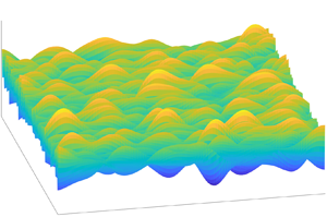
Firstly, we consider the wave evolution over a flat bottom to investigate the effect of initial conditions as reference runs for uneven bottom cases. If we set ${\beta _h} = 0$, (2.13) is equivalent to the 2-D NLS equation in Davey & Stewartson (Reference Davey and Stewartson1974), and the evolution process is constructed by a spatial step in the principal wave direction. The surface elevation is given in discrete 2-D + T form. In figure 2, we give the transient surface elevation $\eta $ at $t = 40{T_0}$ from three random samples with different directional spreads ${\sigma _\theta }$ and the initial BFI = 1 $({\sigma _s} = 0.14)$ at water depth $kh = 5$. The viewing angle is vertical to the horizontal plane, and we use the colour gradient to represent the elevation. The 2-D irregular waves propagate from the left to the right side, and we can figure out the multi-directions from the wavefront lines. As ${\sigma _\theta }$ increases from 0.3 to 0.5, the propagation becomes more divergent in different directions, which makes the wavefront appear to be more discontinuous.

Figure 2. Transient surface elevation $\eta $ at $t = 40{T_0}$ from different directional spreads ${\sigma _\theta }$ with initial BFI = 1, $kh = 5$. (a) ${\sigma _\theta } = 0.3$, (b) ${\sigma _\theta } = 0.4$ and (c) ${\sigma _\theta } = 0.5$.

The initial condition with a random phase in (2.17) helps generate an irregular wave train, and a Monte Carlo simulation is conducted. For a domain in strict-sense stationary (SSS), the statistical properties remain invariant to any shift at any order, and the surface elevation for a 2-D irregular wave at a fixed point will be generally closed to a zero-mean SSS process when the Monte Carlo simulation for random wave phase has enough ensemble size. In this study, we set the ensemble size to 300 and give the average value of kurtosis ${\mu _4}$ and skewness ${\mu _3}$ in time series to each space node. The deciding process of the ensemble size is also discussed in the supplementary materials.

The result in 2-D form can be modified into 1-D form by being averaged again in one space dimension because the statistical significance is uniformly distributed in this 2-D domain. To show the wave evolution process, we take the averaged value on the lateral direction of the principal wave direction and give the Monte Carlo result of the unidirectional wave train and the 2-D wavefield with initial BFI = 0.5 $({\sigma _s} = 0.28)$ for a flat bottom $kh = 7$ to discuss the effect from the directional spread ${\sigma _\theta }$ in figure 3. The result in the unidirectional wave train can be regarded as ${\sigma _\theta } = 0$. As ${\sigma _\theta }$ increases, both kurtosis ${\mu _4}$ and skewness ${\mu _3}$ decrease, which implies the increase of directional spreading disperses the nonlinear interactions in the wave train.

Figure 3. Spatial evolution of kurtosis ${\mu _4}$ and skewness ${\mu _3}$ of surface elevation from directional spread ${\sigma _\theta }$ with initial BFI = 0.5, $kh = 7$ (1-D $({\sigma _\theta } = 0)$, blue; 2-D: red, ${\sigma _\theta } = 0.3$; yellow, ${\sigma _\theta } = 0.4$; black, ${\sigma _\theta } = 0.5$). (a) Kurtosis ${\mu _4}$ and (b) skewness ${\mu _3}$.

For the 2-D propagation in a directional wavefield, both short-time and long-time behaviour of ${\kappa _{40}}$ for a narrowband wave train is related to the directional width and a frequency width (Janssen & Bidlot Reference Janssen and Bidlot2009). We are also interested in the kurtosis distribution at the intermediate stages in freak wave forecasting. Mori et al. (Reference Mori, Onorato and Janssen2011) conducted an asymptotic analysis of ${\kappa _{40}}$, BFI and ${\sigma _\theta }$ by numerical simulation, and gave (2.25) with empirical coefficient $\alpha $. Table 1 shows the ensemble-averaged result of the expected maximum ${\kappa _{40}}$ and mean ${\kappa _{40}}$ at $x \in [20{L_0},30{L_0}]$ from Monte Carlo simulation of the wave model in this study, and gives the empirical coefficients ${\alpha _{max}}$ and ${\alpha _{mean}}$ by (2.25) for maximum ${\kappa _{40}}$ and mean ${\kappa _{40}}$, respectively. Due to different calculation conditions, we give different empirical coefficients from Mori et al. (Reference Mori, Onorato and Janssen2011) $(\alpha = 0.0276)$, and the expected maximum ${\kappa _{40}}$ is significantly larger than their prediction. Nevertheless, the result from $kh = 7$ shows that the increase of ${\sigma _\theta }$ and the decrease of BFI lead to the decrease of both maximum and mean ${\kappa _{40}}$, but the change in empirical coefficient $\alpha $ represents that ${\kappa _{40}}$ is not strictly inversely proportional to ${\sigma _\theta }$ as in (2.25), and the case from different initial BFI will ask for a different $\alpha $. The value of ${\alpha _{mean}}$ for mean ${\kappa _{40}}$ at $kh = 7$ is better than ${\alpha _{max}}$ to describe the kurtosis of the wavefield, and its value is around 0.09~0.14. When the water depth becomes shallow ($kh = 5$, 3, 1.1), (2.25) is no longer applicable and ${\alpha _{mean}}$ and ${\alpha _{max}}$ significantly decrease. For $kh = 1.1$, the increase of ${\sigma _\theta }$ leads to the increase of ${\kappa _{40}}$ and ${\alpha _{mean}}$, which seems anomalous. The behaviour of ${\kappa _{40}}$ further indicates that the occurrence of extreme wave height in medium and shallow water cannot only be predicted by the four-wave interaction as in deep water. The contribution from water depth becomes important, especially in shallow water, and the simulation over a changing depth may reveal this process more effectively.

Table 1. The ensemble-averaged ${\kappa _{40}}$ dependence on BFI and ${\sigma _\theta }$ at different $kh$.

3.3. Evolution of modulated wave over uneven bottoms

This section considers Monte Carlo simulation of the 2-D wave model for uneven bottoms. The variation in the bottom topography brings about the spatial inhomogeneity in the dispersion, which reflects in both second-order and third-order effects. Our numerical model by (2.13) assumes the depth mildly changes in the principal wave direction, and the bottom topography does not vary in its lateral direction. Therefore, the statistical properties remain stationary on the y-axis but vary on the x-axis.

As a simulation of the bottom topography from offshore to onshore, we set the depth to slowly decrease from a medium-water depth to shallow water. In previous research (e.g. Kashima & Mori Reference Kashima and Mori2019; Li et al. Reference Li, Draycott, Zheng, Lin, Adcock and Bremer2021; Lyu et al. Reference Lyu, Mori and Kashima2021), the abrupt change in depth or slope led to significant local peaks in ${\mu _3}$ and ${\mu _4}$ due to the after effect. Usually, the water depth decreases in a smoother way in the natural seabed. On the other hand, the local peak caused by this unusual topography is so significant that it may cover the difference caused by the directional effect. To make our simulation closer to the natural seabed, we adjust the sloping region in figure 1 between A and B to become smoother and to continuously decrease, as shown in figure 4. The sloping region is divided into two parts by the dividing line C at $kh = 1.2$: the depth linearly decreases with a slope ${\gamma _s}$ from $kh = 5$ to $kh = 1.2$; the depth decreases with a decaying slope ${\gamma ^{\prime}_s} = {\gamma _s}{(h/1.55)^{40}}$ from $kh = 1.2$ to $kh = 1.1$. In the shallow-water area, the derivative of the decreasing depth is approximately continuous, and we set ${\gamma _s} = 0.05$, 0.02, 0.01 to ensure the depth changes very mildly under the assumption $h^{\prime}(x)\sim O({\varepsilon ^2})$.

Figure 4. The variation of water depth $kh$ on the bottom topography with ${\gamma _s} = 0.02$.

Figures 5 and 6 shows the averaged values of kurtosis and skewness from the Monte Carlo simulation of the bottom type in figure 4. In figure 5, we give the averaged kurtosis ${\mu _4}$ in 2-D form at the different directional spread ${\sigma _\theta }$ and slope angle ${\gamma _s}$ with initial BFI = 0.4 $({\sigma _s} = 0.35)$. Comparing the result from different ${\sigma _\theta }$ in figure 5(a–c), we find that ${\mu _4}$ decreases in the deep-water depth but increases in the shallow water when the initial directional spreading ${\sigma _\theta }$ increases from 0.3 to 0.5, which shows that the same phenomenon results in a flat bottom in § 3.1. In the medium-water depth region between locations A and C, ${\mu _4}$ decreases with the decrease of water depth, and it rebounds at the end of the constant sloping region (location C) where $kh = 1.2$. In the region between C and B, where the slope angle mildly decreases, ${\mu _4}$ decreases and becomes stable at the same level as the final flat bottom in shallow water $kh = 1.1$. The evolution of ${\mu _4}$ indicates that the directional dispersion effect decreases the occurrence probability of freak waves in deep and medium water but increases it in shallow water. As the wave propagates from the medium water to shallow water, the wave evolution is significantly affected by the bottom topography, and the 1-D result in figure 5(d) clearly gives the rebound of ${\mu _4}$ due to the slope angle. To further study the effect from the bottom topography, we give the mean ${\mu _4}$ at ${\gamma _s} = 0.02$ and ${\gamma _s} = 0.01$ with initial BFI = 0.4 and ${\sigma _\theta } = 0.3$ in figures 5(e) and 5( f). The result shows that the rebound of ${\mu _4}$ decreases as the bottom change become milder, and figure 5(g) provides the variation of ${\mu _4}$ in the principal wave direction in one dimension. Comparing ${\mu _4}$ over uneven bottoms between the unidirectional wave train and the 2-D wavefield, we find the slope angle similarly affects the wave evolution. However, its contribution is more significant in two dimensions due to the dispersion effect in the four-wave interaction, which implies the second-order effect plays a more important role in a directional 2-D wavefield.

Figure 5. Mean kurtosis of surface elevation $\eta $ for uneven bottoms at different directional spreads ${\sigma _\theta }$ and slope angles ${\gamma _s}$ with initial BFI = 0.4 (blue, ${\sigma _\theta } = 0.3$; red, ${\sigma _\theta } = 0.4$; yellow, ${\sigma _\theta } = 0.5$; g: blue, ${\gamma _s} = 0.05$; red, ${\gamma _s} = 0.02$; yellow, ${\gamma _s} = 0.01$). (a) ${\sigma _\theta } = 0.3$, ${\gamma _s} = 0.05$, (b) ${\sigma _\theta } = 0.4$, ${\gamma _s} = 0.05$, (c) ${\sigma _\theta } = 0.5$, ${\gamma _s} = 0.05$, (d) ${\sigma _\theta } = 0.3$, 0.4, 0.5, ${\gamma _s} = 0.05$, (e) ${\sigma _\theta } = 0.3$, ${\gamma _s} = 0.02$, ( f) ${\sigma _\theta } = 0.3$, ${\gamma _s} = 0.01$ and (g) ${\sigma _\theta } = 0.3$, ${\gamma _s} = 0.05$, 0.02, 0.01.

Figure 6. Mean skewness of surface elevation $\eta $ for uneven bottoms at different directional spreads ${\sigma _\theta }$ and slope angles ${\gamma _s}$ with initial BFI = 0.4 (blue, ${\sigma _\theta } = 0.3$; red, ${\sigma _\theta } = 0.4$; yellow, ${\sigma _\theta } = 0.5$; g: blue, ${\gamma _s} = 0.05$; red, ${\gamma _s} = 0.02$; yellow, ${\gamma _s} = 0.01$). (a) ${\sigma _\theta } = 0.3$, ${\gamma _s} = 0.05$, (b) ${\sigma _\theta } = 0.4$, ${\gamma _s} = 0.05$, (c) ${\sigma _\theta } = 0.5$, ${\gamma _s} = 0.05$, (d) ${\sigma _\theta } = 0.3$, 0.4, 0.5, ${\gamma _s} = 0.05$, (e) ${\sigma _\theta } = 0.3$, ${\gamma _s} = 0.02$, ( f) ${\sigma _\theta } = 0.3$, ${\gamma _s} = 0.01$ and (g) ${\sigma _\theta } = 0.3$, ${\gamma _s} = 0.05$, 0.02, 0.01.

In figure 6, we give skewness ${\mu _3}$ in the same form as ${\mu _4}$ in figure 5 at the same condition. Different from ${\mu _4}$, ${\mu _3}$ does not influence directional spread from figure 6(a–d) due to the unchanging second-order nonlinear interaction. When the bottom topography changes, figure 6(e–g) shows that ${\mu _3}$ increases as the water depth become shallow. This process will slow down if the slope angle becomes mild, but it only means ${\mu _3}$ is determined by the water depth $kh$ and the change from slope angle ${\gamma _s}$ has little influence. Different from the unidirectional wave train, ${\mu _3}$ in the 2-D wavefield is basically only determined by the variation in dispersion due to depth change, and is hardly affected by the local bathymetry effect. When the wave trains propagate into shallow water, ${\mu _3}$ increases with the increase of wave steepness $\varepsilon $.

3.4. Quantitative analysis of the extreme wave height

In §§ 3.2 and 3.3, the evolutions of the nonlinear resonant interactions have been discussed with the bathymetry effect at different water depths. Parameters ${\mu _4}$ and ${\mu _3}$ represent different nonlinear mechanisms, and they show different characteristics on the directional wavefield over an uneven bottom. However, the final result of the occurrence of extreme wave height is their combined effect, and we cannot simply give the estimation until giving a quantitative analysis of the distribution of surface elevation $\eta $.

In figure 7, we give the expected maximum wave height ${H_{max}}$ and maximum wave crest ${\eta _{max}}$ in the principal wave direction. In the same form as ${\mu _4}$ and ${\mu _3}$ in figures 5 and 6, ${H_{max}}$ and ${\eta _{max}}$ are counted from the time series sampling data at a fixed point in the 2-D wavefield, and their ensemble-averaged value is given by Monte Carlo simulation. We make the wave height dimensionless by taking ${H_{max}}/{\eta _{rms}}$ and ${\eta _{max}}/{\eta _{rms}}$, and continue to write them as ${H_{max}}$ and ${\eta _{max}}$ for convenience. The result contains the wave train with different directional spreadings ${\sigma _\theta } = 0.3$, 0.4, 0.5 over the bottom topography ${\gamma _s} = 0.05$, 0.02, 0.01, and the theoretical result from the linear model (Rayleigh distribution) and the numerical result from the second-order bound wave model in ${\sigma _\theta } = 0.3$, ${\gamma _s} = 0.05$ are given for comparison. The Rayleigh distribution can be referred to as the standard linear narrow-banded wave theory in Goda (Reference Goda1970, Reference Goda2000), in which the wave height H follows the Gaussian distribution and the exceeding probability ${P_m}({H_{max}})$ follows

(3.3)\begin{equation}{P_m}({H_{max}}) = 1 - \exp ( - {N_0}\,{\textrm{e}^{ - H_{max}^2/8}}),\end{equation}

where the number of waves ${N_0} = 40$ in our simulation. From deep water to shallow, ${H_{max}}$ in 2-D model monotonically decreases with the water depth in comparison with the second-order model. Similar with ${\mu _4}$, the peak of ${H_{max}}$ is suppressed by the increase of ${\sigma _\theta }$ in deep water but is enhanced in shallow water. However, there is no significant change in the slope. In figure 7(b), the ${\eta _{max}}$ significantly increases in shallow water, and the local peak reflects the contribution from the slope. Even when the bottom changes in a relatively continuous process, this local peak still occurs, and is consistent with the variation of ${\mu _4}$. Different from ${H_{max}}$ in shallow water, the increase of ${\eta _{max}}$ is related to ${\mu _3}$, in keeping with the general deformation of waves in the shoaling process. In the Rayleigh distribution, ${H_{max}}$ and ${\eta _{max}}$ are independent of the bathymetry. The linear model underestimates ${H_{max}}$ in deep water and overestimates it in the shallow water, and significantly underestimates ${\eta _{max}}$. As a result of the second-order bound wave model, ${H_{max}}$ is hardly affected by the bottom topography and ${\eta _{max}}$ is determined by wave steepness. Comparing different models, the present model provides more consideration of the different effects of the four-wave interaction at various depths. Comparing the result in figures 5–7, we find the rebound of ${\mu _4}$ at location C does not reflect in ${H_{max}}$ but shows in ${\eta _{max}}$, which implies the wave height distribution at this area is more determined by the topography effect at second order rather than the four-wave interaction at third order.

Figure 7. Ensemble-averaged expected maximum wave height and free surface elevation distribution at initial BFI = 0.4 from different ${\sigma _\theta }$ and ${\gamma _s}$ (present model: black, ${\sigma _\theta } = 0.3\;{\gamma _s} = 0.05$; blue, ${\sigma _\theta } = 0.4\;{\gamma _s} = 0.05$; red, ${\sigma _\theta } = 0.5\;{\gamma _s} = 0.05$; yellow, ${\sigma _\theta } = 0.3\;{\gamma _s} = 0.02$; grey, ${\sigma _\theta } = 0.3\;{\gamma _s} = 0.01$. Second-order model: dotted, ${\sigma _\theta } = 0.3\;{\gamma _s} = 0.05$. Rayleigh distribution: green line). (a) Maximum wave height ${H_{max}}$ and (b) maximum wave crest ${\eta _{max}}$.

When concentrating on the freak wave problem, only the expected value is insufficient to estimate the extreme case. Therefore, we integrate the distributions of ${H_{max}}$ and ${\eta _{max}}$ at each section in the principal wave direction. If we follow the common definition of the freak wave as the wave height exceeds the significant wave height by a factor two, then the occurrence probability of a freak wave height is $P_f(H_{max})$ when ${H_{max}} > 8{\eta _{rms}}$ and the corresponding probability estimated by the wave crest is $P_f(\eta_{max})$ when ${\eta _{max}} > 4{\eta _{rms}}$ under the standard linear narrow-banded wave theory from Goda (Reference Goda1970, Reference Goda2000) (f, freak wave). Figure 8 calculates the probabilities as mentioned above and gives the fit curves through the tenth-order polynomial. A little different from figures 5–7, the horizontal axis is set to be the water depth $kh$ in figure 8, so we can more easily check the effect from different ${\gamma _s}$ at the same depth. In figure 8(a), $P_f(H_{max})$ monotonically decreases with the water depth as expected ${H_{max}}$, but more details can be given: in relatively deep water such as $kh > 4$, the convergence of $P_f(H_{max})$ becomes worse, which implies the variance of surface elevation significantly rises; for the shallow water $kh < 2$, the increase of slope angle ${\gamma _s}$ enhances the probability of freak waves; the directional spreading ${\sigma _\theta }$ plays a more important role in deep water, but bottom topography has a greater impact in shallow water. Compared with figure 8(a), $P_f(H_{max})$ in figure 8(b) is much larger than $P_f(H_{max})$ in general, and it experiences a process of descending, ascending and descending again with the decrease of $kh$. In the linear model, the probabilities in figure 8(a,b) show the same result, and their deviation from current models corresponds to the evolution in figure 7. The result from the second-order bound wave model continues to show a strong correlation with wave steepness $\varepsilon $, and it gives an abnormal enhancement in both $P_f(H_{max})$ and ${P_f}({\eta _{max}})$ in very shallow water after the slope section, which is not consistent with the natural state and experiments.

Figure 8. Occurrence probability of the freak wave in wave height and free surface elevation distribution at initial BFI = 0.4 from different ${\sigma _\theta }$ and ${\gamma _s}$ (present model: black, ${\sigma _\theta } = 0.3\;{\gamma _s} = 0.05$; blue, ${\sigma _\theta } = 0.4\;{\gamma _s} = 0.05$; red, ${\sigma _\theta } = 0.5\;{\gamma _s} = 0.05$; yellow, ${\sigma _\theta } = 0.3\;{\gamma _s} = 0.02$; grey, ${\sigma _\theta } = 0.3\;{\gamma _s} = 0.01$. Second-order model: dotted, ${\sigma _\theta } = 0.3\;{\gamma _s} = 0.05$. Rayleigh distribution: green line). (a) probability of ${H_{max}} > 8{\eta _{rms}}$ and (b) probability of ${\eta _{max}} > 4{\eta _{rms}}$.

In figures 9 and 10, we give the wave height distribution in CDF in logarithmic coordinates at specific sections at different water depths. We choose five sections on the sloping region in figure 4: S1 (dashed line A in previous figures) where $kh = 5$; S2 where $kh = 3$; S3 where $kh = 2$; S4 (dashed line C in previous figures) where $kh = 1.2$; S5 (dashed line B in previous figures) where $kh = 1.1$. Figure 9 shows the CDF of ${P_m}({H_{max}})$ from the same conditions as before compared with the Rayleigh distribution (i.e. linear distribution). As the water depth decreases from S1 to S5, the occurrence probability of ${H_{max}}$ decreases from the comparison with the Rayleigh distribution (the linear distribution model does not change with water depth). The nonlinear model gives a higher exceeding probability of extreme events than the linear distribution in deep water (S1) but lower in shallow water (S4, S5). They have a similar prediction of wave heights distribution in medium-water depth (S2, S3). In S1–S3, the increase of directional spread ${\sigma _\theta }$ leads to the decrease in the probability of exceeding ${H_{max}}/{\eta _{rms}} > 6$. However, in shallow-water depth (S4, S5), the effect of ${\sigma _\theta }$ is very limited or even becomes opposite. The effect from ${\gamma _s}$ works mainly in the shallow region, and focuses on the distribution of larger values (i.e. the occurrence of a ‘freak wave’). The result from the second-order bound wave model is hardly affected by the water depth from S1 to S4, but increases in very shallow water S5, especially for the occurrence of extreme values, and exceeds the result from the present model. In figure 10, we give the CDF of ${P_m}({\eta _{max}})$ in the same form. Basically, ${P_m}({\eta _{max}})$ shows a similar variation as ${P_m}({H_{max}})$ under the effect from ${\sigma _\theta }$ and ${\gamma _s}$, but ${P_m}({\eta _{max}})$ markedly exceeds the Rayleigh distribution, which indicates that the wave deformation makes the wave crest exceed half the wave height due to the nonlinear effect. In shallow water, this deviation becomes more obvious for a smaller value ${\eta _{max}}/{\eta _{rms}} > 3$, even the extreme case decreases, which indicates the second-order nonlinear effect significantly rises due to the bottom topography change.

Figure 9. Exceedance probability of maximum wave height ${H_{max}}$ at initial BFI = 0.4 from different ${\sigma _\theta }$ and ${\gamma _s}$ (present model: black cross, ${\sigma _\theta } = 0.3\;{\gamma _s} = 0.05$; blue, ${\sigma _\theta } = 0.4\;{\gamma _s} = 0.05$; red, ${\sigma _\theta } = 0.5\;{\gamma _s} = 0.05$; yellow, ${\sigma _\theta } = 0.3\;{\gamma _s} = 0.02$; grey, ${\sigma _\theta } = 0.3\;{\gamma _s} = 0.01$. Second-order model: black circle, ${\sigma _\theta } = 0.3\;{\gamma _s} = 0.05$. Rayleigh distribution: green line); (a) S1 $(kh = 5)$, (b) S2 $(kh = 3)$, (c) S3 $(kh = 2)$, (d) S4 $(kh = 1.2)$ and (e) S5 $(kh = 1.1)$.

Figure 10. Exceedance probability of maximum wave crest ${\eta _{max}}$ at initial BFI = 0.4 from different ${\sigma _\theta }$ and ${\gamma _s}$ (present model: black cross, ${\sigma _\theta } = 0.3\;{\gamma _s} = 0.05$; blue, ${\sigma _\theta } = 0.4\;{\gamma _s} = 0.05$; red, ${\sigma _\theta } = 0.5\;{\gamma _s} = 0.05$; yellow, ${\sigma _\theta } = 0.3\;{\gamma _s} = 0.02$; grey, ${\sigma _\theta } = 0.3\;{\gamma _s} = 0.01$. Second-order model: black circle, ${\sigma _\theta } = 0.3\;{\gamma _s} = 0.05$. Rayleigh distribution: green line); (a) S1 $(kh = 5)$, (b) S2 $(kh = 3)$, (c) S3 $(kh = 2)$, (d) S4 $(kh = 1.2)$ and (e) S5 $(kh = 1.1)$.