Introduction
A method for measuring the mass balance for a small region of an ice sheet is needed, The usual method is to compare snow input with horizontal output (Reference Mosley-Thompsone.g. Kostecka and Whillans, 1988; Reference Whillans and BolzanWhillans and Bindschadler, 1988; Reference Bindschadler, Vornberger and ShabtaieBindschadler and others, 1993) but areas on the order of 10+ km2 must be considered so that uncertainties associated with the depth variation in velocity or the boundaries of the catchment area do not dominate the calculation. New methods use repeat satellite-radar altimetry to observe surface-elevation change (Reference ZwallyZwally, 1984; Reference Wingham, Rapley and MorelyWingham and others, 1993). The potential problems with this method are associated with signal penetration into the firn, ambiguity due to beam width and off-pointing, and uncertainties in satellite orbits and track positioning. Repeat laser altimetry from aircraft is another promising possibility. Both new methods have great merit in the ability to obtain locally specific changes over large regions. However, these techniques are limited in that they cannot distinguish between time changes in ice mass and changing firn density. Firn density may be expected to change most importantly at shallow depths, due, for example, to secular changes in mass loss by vapor transport, or especially warm or cool summers affecting densification. Also, it is well established that accumulation rate varies significantly over short time-scales (Reference Mosley-ThompsonMosley-Thompson, 1980; Reference Jouzel, Merlivat and LoriusJouzel and others, 1983), such as the several years between altimetric observations. Because they are linked strictly to the surface, remote observations arc especially sensitive to such changes. A locally applicable method is needed that is less affected by rapid, short-duration variations and that applies to long time-scales. Such measurements are valuable in themselves and would also provide calibration, or fiducial sites, for altimetric techniques.
The method proposed here, using the Global Positioning System (GPS), offers a rapid and precise local measure of ice-thickness change. The technique uses post-processing of simultaneous satellite tracking from receivers at remote sites on the ice sheet and at reference sites on rock to provide accurate horizontal and vertical positions for the remote sites. Markers are planted in the firn or ice at the remote site. Re-occupation at a later time to observe change in position of the marker yields a vertical velocity related to firn accumulation and rate of ice-thickness change. The extent to which the vertical velocity may not be compensated by the accumulation rate is a measure of ice-thickness imbalance.
Theory
An ice sheet might not be in steady state for two reasons. First, there may have been a change in the balance between surface-accumulation rate and ice flow and basal melting/freezing. This results in a net mass imbalance in which the downward motion of the ice is not being exactly matched by new addition of ice at the top. This difference, the net change in ice thickness,is the objective of the work here. Secondly, there may have been a change in firn properties or accumulation rate that affects the rate of firn settling. We seek to avoid this complication by placing the markers as deeply as possible in the firn so as to be less affected by short-term fluctuations in firn temperature and accumulation rate. Ideally, the markers should be set in solid ice but depths of some tens of meters may be all that is feasible.
As firn accumulates, it settles and thereby densifies. Each particle is continuously being displaced downward. If the accumulation rate, b, is constant, the firn moves downward at the rate: -b /ρ(z), where density, ρ, increases with depth, z. This relation is known as Sorge's law (Reference PatersonPaterson, 1981, p. 16). The negative sign indicates downward motion.
A marker in the firn moves downward with this firn settling and is also affected by any rate of change of thickness of the ice beneath. This quantity, the long-term rate of thickness change, H, is added to the settling velocity to obtain the vertical velocity of the marker, ω:
No separate account of basal melting or basal freezing need be taken. Any vertical velocity due to crustal motion has been neglected.Equation (1) is applied to measured velocities of markers planted at specific depths (and densities) and solved to compute a rate of ice-thickness change, H, from each marker. If markers at several depths are used, a linear relationship is expected between wand 1/ρ if Sorge's law applies.
A part of the vertical motion of the marker is due to down-slope ice flow. If the surface slope is constant with time, the effect of down-slope flow is removed by considering not quite the vertical velocity of markers but the surface-perpendicular component of velocity. For most ice sheets, slopes are on the order of 0.002, so the directions of vertical and surface-perpendicular are very similar.
Field method
Data collection has three elements: 1. Long-distance tie between remote site and stable GPS stations 2. Emplacement of deep vertical velocity markers and their survey connection to the long-distance tie. 3. Collection of ancillary data: a. Surface slope. b. Profile of firn density. c. Local accumulation rate Its application at Amundsen-Scott South Pole Station and Byrd Station is discussed here. Neither site has a complete suite of measurements. At South Pole, a new experiment was established in January 1993. Several markers were placed and surveyed once, surface slope was measured and firn-density profiles were recorded for each marker hole. The markers will be re-surveyed for rate of thickness-change calculations after several years. All CPS and density-profile discussions refer to this site. The firn settling evaluation is drawn from old surveys near Byrd Station (Reference GowGow, 1968; Reference WhillansWhillans, 1991). There is no survey tie to a fixed location for the Byrd Station data.
Long-distance tie to South Pole
GPS data are continually recorded by a receiver at Amundsen-Scott South Pole Station and by another, on rock, at McMurdo Station on Ross Island. The separation distance is about 1300km. Data are collected using geodetic quality receivers, sampling at a 30 s interval. Both L1 and L2 CPS frequencies are recorded so that ionospheric corrections can be made. Calculations for such long-distance ties require 24 h or longer data sets, precise orbits and orbit-relaxation techniques. At present, solutions of long base lines between stations on rock and ice are not complete. However, calculations for positions of receivers on rock are accurate to 0.01m (personal communication from P.J. Morgan, University of Canberra, 1993). It is possible that difficulties in accounting for the motion of ice during the CPS observations may degrade the results to about 0.05m.
Deep markers at South Pole
The vertical motion markers are distant enough from long-standing camps that artificial effects due to snow drifting or compaction are avoided. A minimum distance is 2-3km, the response distance of katabatic wind to a disturbance (Reference WhillansWhillans, 1975). The present site (Fig. 1) is about 7km along 1300 E from the station structures. The prevailing wind is from about 20°E. The site is too small to present a drifting problem of its own and was constructed with as little disturbance to the area as possible

fig. 1 Location of monitoring site installed near South Pole. Deep markers are Placed in a ring at the circled asterisk. Other asterisks indicate stations of the GPS surface-slope survey. Contours (in m) are of surface height relative to the marker site.
The vertical motion markers are long poles, spaced several meters apart, planted at depths of 4, 6, 8, 10, 12, 14, 16 and 20m within the firn during January 1993. Observations at multiple depths (and densities) are required to test the validity of Sorge's law in Equation (1). For each marker, a hole was hand-augered to the desired depth. Long poles were constructed by connecting sections of 19mm diameter hollow-steel conduit. A steel can 10.1m diameter) filled with slush was frozen on to the bottom of each long pole as a footing to prevent penetration below the bottom of the hole. In effect, it is the motion of the steel can that is being monitored. A plywood cap is placed around each pole and over the hole, and buried with snow to prevent filling by windblown snow. Thus, the hole remains open and the pole is not gripped by firn at any depth other than the hole bottom. This concern is also assuaged by the use of steel conduit with nearly flush connectors whose smooth surface is not easily gripped by firn. The poles flex slightly as constrained by the hole walls. The amount of flexure does not change with time. The elevations of the pole tops are measured over a span of years.
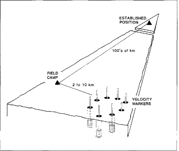
A static GPS technique is used to make the connection between the marker site and the long-distance tracker at Amundsen-Scott South Pole Station. Dual-frequency phase observations of an hour or more are made with an antenna placed directly on top of one of the marker poles. Post-processing produces a relative position accurate to 0.01m. The positions of the other markers are surveyed relative to the first, using the stop-and-go kinematic GPS technique (Reference Hulbe and WhillansHulbe and Whillans, 1993) and by optical levelling. For these GPS surveys, a fixed reference receiver is placed on the marker pole which has been surveyed relative to the South Pole receiver. With the fixed receiver continually tracking phase of the GPS signals, a second antenna, also continually tracking, is placed, in turn, on each of the other pole tops. Ten or more epochs of 5 s interval data are collected on each marker. Differential post-processing determines the positions of the pole tops with respect to the marker used as the fixed location. Because only the pole tops are used for the survey, antenna heights are zero. Thus, problems related to changing surface conditions and setting of the antenna are avoided. Similar kinematic GPS surveys elsewhere in Antarctica (Reference Hulbe and WhillansHulbe and Whillans, 1993) yield accuracies of 0.005m km-1 or better for horizontal and vertical components. The optical levelling for the example used here from near Byrd Station is internally consistent to 0.002m. The relationships of survey steps, from a permanent site on rock to vertical motion markers, are sketched in Figure 2.

fig. 2 The positions of firn markers are linked to a field camp and to a stable site.
Ancillary data
Surface slope at South Pole
The stop-and-go kinematic CPS technique is used to determine surface slope. A receiver was left tracking at the marker site and a vehicle carrying a second GPS antenna drove a 4 km by 4km grid around the site, stopping about every 500m. Five ten epochs of 5 s interval data were collected at each stop for a precise position calculation. The sites of such stops are shown in Figure 1. The area surveyed is large enough to represent accurately the local surface and enough points are observed to avoid biasing by local surface micro-relief.
At this site, the slope is 2.5m/1000m in the flow direction (known to be 8.5m a-1, 40° W at the station (United States Geological Survey, 1976)). Slope calculations along repeated grid lines agree to within 10%, leading to our estimate of 0.25 x 10⁻³ for the slope error.
The local surface topography may change between observation epochs. For example, surface slope may change or topographic features may migrate through the surveyed area. Such phenomena may indicate non-steady ice flow. This possibility should be assessed by repeating the local surface topography survey for each epoch.
Firn-density profile at South Pole
Firn density at the depth of each marker is needed. This is obtained from cores retrieved when the holes are drilled
Errors in density are mainly due to uncertainties in core diameter, which affect each density by about 2%. Uncertainties and the possibility of horizontal variation in density are evaluated from the reproducibility of density profiles. The standard error is 1% at 6m depth and 1.6% at 10m depth for the cores at the South Pole site, which are within 20m of one another. Such variability is within measurement uncertainty. A further estimate of density precision is obtained from the scatter of values in the test of Equation (1), as discussed in relation to Figure 3. The correlation coefficient for the regression suggests a density uncertainty of 3%.

fig. 3 Vertical velocity of marker versus inverse density at marker depth. The data are from deep anchors at several locations near Byrd Station. The observation interval is about 2years.
Uncertain core break and lost sections of core cause some uncertainty in the depths of density values. The depth uncertainty is calculated following Reference Whillans and BolzanWhilians and Bolzan (1988) and is about 0.0 15m. This is relatively unimportant
Accumulation rate
The accumulation rate is best obtained independently, at the marker site, using stratigraphic methods, such as the detection of horizons of gross β activity or dust layers in ice cores.Reference Whillans and Bindschadler Whillans and Bindschadler (1988) found that the largest error sources are with the densities of samples between the dated horizons. which affect accumulation rates by about 2% (Table 1, note II), and spatial irregularities in the strata due to sastrugi, which can affect accumulation rate by several per cent (Reference WhillansWhillans (1975) calculated about 0.01 ma-1 along the Byrd Station Strain Network). Note that density error affects the calculation in two places, first, at the marker depth (see above) and here, where the depth-integrated density between dated strata is needed. Spatial variability m accumulation rate is important.
Table 1. Uncertainties in mass-halance calculation

Notes
(1) Vertical position from a static calculation between a GPS receiver on the ice sheet (at Amundsen Scott South Pole Station; and an established GPS receiver (McMurdo Station, on rock).
(2) Vertical position of a vertical motion marker. made with a GPS tie relative to the field camp receiver (at Amundsen--Scott South Pole Station).
(3) The root of summed squares of the position errors (1) and (2).
(4) From a kinematic GPS survey around the marker site.
(5) From the same survey operation described in notes (1) and (2).
(6) The surface-perpendicular velocity is the dot product between the unit Vector normal to the snow, surface, n, and ice velocity u. That is: w=u.n = uxnx + uyny + uz,nz, in which the subscripts identify the vector components. This is simplified by considering only the vertical, z, and along-flow x, components. Let α represent slope angle. Then w = ux sinα + uz, cosα. Error propagation using this equation links standard errors in each quantity. The effect of error in slope is (ux. cos α + uz, sin α)σx and considering that α « 1 this becomes (ux+auz)σx This is evaluated, assuming a 5 year observation interval using estimates appropriate for South Pole ux͌8.5 ma1a͌2.5×10³,uz͌0.1 ma1 and σx =2 x 10⁴, to provide the value in the table.
(7) Density is calculated using ρ = 4M/LπD2 where M represents sample mass, L is sample length and D is sample diameter. Diameter uncertainty is the most limiting factor (Whillans and Bindsehadler, 1988). Neglecting other contributions, the error in density is ρρ = (8M / Lπ D3)ρD = (2ρ/D)ρD where ρD represents the error in diameter measurement. Representation values are (ρ = 0.5 Mg m 3, D = 0.076 m, ρD =0.001 m By this error propagation. ρρ is 0.013 .Mgm3. An independent estimate comes limn the standard deviation of the regression fit in Figure 2. That is 3% of 0.015 Mgm3. This slightly more pessimistic value is reported in Table 1.
(8) From Equation (2), the effect is: (b/ρ2)σρ The value in Table 1 is calculated with b = 0.14Mgm 2a 1 (typical for Byrd Station).
(9) Error obtained from the statistics of the regression in Figure 2.
(10) From Equation (2), the effect is σb/ρ.
(11) There are four important sources of error in accumulation rate determined by core stratigraphy. Two stem from data collection and two from natural phenomena. The first two uncertainties in accumulation rate are due to uncertainties in core-diameter measurement. The accumulation rate from a single core is calculated from b = 1/T Σ 4M/πD2 in Which T represents the time interval between dated strata. The sum is taken over N samples. The mass and diameter of each sample along the core are represented by M and D, respectively. Accuracy is almost entirely limited by the diameter in which there may be (1) random and (2) systematic, errors. Random measurement errors in diameter,σrandom affect the accumulation rate according- to σDrandom = (2√Np/TD)σDrandom systematic bias in diameter σDsystematic affects accumulation rate according to. σbsystematic=(2b/D)σDsystematic
Measurement errors are estimated for the case of accumulation rate determined by the detection of, β fall-out horizons, a common method. A core is augered to a depth of 15-20m to find the stratum containing- the start of radioactive fall-out in 1955. Typical values from such an analysis are N=40, T=.40a, D=0.076m, ρ= 0.5 Mgm 3. b= 0.14:Mgm 2a 1 σDrandom = 0.001 m. This leads to σbrandom =0.002 Mg m 2a 1 and σbsystematic=0.004 Mg m 2 a 1.
A third uncertainty arises because depositional strata are horizontally variable on the 10m scale due to sastrugi. Thus, there is a sampling error. Letting ( σs represent sastrugi roughness (for simplicity. taken to be the same for both the upper and lower strata), the associated standard error in accumulation rate is σbsastrugi= (√2/T)σ s. Using a value of 0.02m for σs as reported for near Byrd Station, (Whillans, 1978), the sastrugi effect is 0.0006 Mg m 2 a 1.
The fourth uncertainty arises from short-term variability in accumulation rate, as discussed in the text under “long-term significance”. The .standard error at South Pole due to this is 0.0038 Mg m 2 a 1 Combining all four sources of error, the net standard error is 0.006 Mg m 2 a 1.
(12) The solution of Equation (2).
Reference Jouzel, Merlivat and LoriusJouzel and others (1983) compared independent accumulation- rate determinations near South Pole. They found a variability of 30-40% between authors. All these authors assumed that spatial variations in density are unimportant and, indeed, the variations seem too large to be due to density. Reference WhillansWhillans (1978) found accumulation rates along the 168 km long Byrd Station Strain Network to vary by 14-40% over distances of about 10 km. These works point to the importance of obtaining the accumulation rate from cores taken at the marker site
The long-term accumulation rate may also be obtained from firn settling as a result of the solution of Equation (1) as discussed below.
Firn settling
An application near Byrd Station is illustrated in Figure 3 (Reference Whillansfrom Whillans, 1991). The markers were planted at depths ranging to 25 m and surveyed with optical techniques. Densities are obtained from Reference GowGow (1968). The surveying was done long ago and so there is no connection to a fixed location. Thus, there is an unknown constant error in the vertical velocity, W, and the data cannot be used to compute mass balance. However, they can be used to demonstrate a test of the model of firn settling. In Figure 3, measured vertical velocities are plotted against inverse density at marker depth. If Sorge's law applies, Equation (1) predicts a straight line. This seems to be the case, which supports the assumption that firn densification is steady. That is, past changes in firn temperature, or in the rate of loading by new snow, or in vapor transfer within the firn pack are not important. Should the relation not be linear, there would be some complicating process, which must be identified in order to determine which marker velocities are most meaningful.
A linear regression on the data of Figure 1 yields an accumulation rate (the slope of the best-fit line) of 0.137 Mg m2a1. The standard error on this estimate is 0.04 ),Mg m2a1 the scatter is taken as due to error in density and all values are assigned equal weight. This error is larger than the error associated with accumulation rate obtained stratigraphically. Therefore, it seems prudent to obtain the accumulation rate from stratigraphic studies on an ice core taken at the measurement site, rather than rely on this use of Sorge's law.
The accumulation rate derived from the regression is within the range of other estimates from nearby sites. A rate of 0.140 Mg m 2 a 1 is obtained for the interval 1925 60 from pit and core work at Old Byrd Station (Gow, 1961). A rate of 0.144 Mg m 2 a 1 is obtained for the interval 1930-61 from pit and core work at New Byrd Station (Reference KoernerKoerner, 1964). And, a rate of 0.104 Mg m-2 a-1 is obtained for the interval 1925-63 from a 10m pit at New Byrd Station (Reference CameronCameron, 1971). This agreement supports the general soundness of the method and Equation (1).
Long-term significance
The rate of snow accumulation varies with time, yet the motion of the glacier is linked to the response time of the glacier, which is thousands of years. An accumulation rate record spanning thousands of years is preferred
The time variability in accumulation rate is estimated from a long time series. There are 911 yearly accumulation rate values from a long core collected at South Pole (Reference Mosley-ThompsonMosley-Thompson, 1980, table 13). The values come from the spacing of dust layers and a density profile of uncertain accuracy. The standard deviation of 40 year averages is 0.0038Mgm-2a-1 (40 years is comparable to the time-scale applicable to accumulation rate from gross β activity). This standard deviation is a measure of the confidence with which accumulation rate from a single short core can be used to estimate long-term accumulation rate.
This standard error is similar to the accumulation-rate calculation error (0.0045 Mg m -2 a -1]; Table 1, note 11). For South Pole, the assumption that accumulation rate is constant, as required by Sorge's law, seems to be about as limiting as errors in field measurements
Error analysis
The rate of ice-thickness change,H,is obtained. By solution of Equation (1). The standard error for H is given by:
where 2σz 2 represents the combined vertical positioning error for surveys at two different epochs, σb represents the error in accumulation rate, up represents the error in density at marker depth and !1t represents the time interval between surveys. Each contribution is addressed in Table 1.
The largest uncertainty in the calculation is due to difficulties in obtaining a precise value for the long-term accumulation rate, σb, In that, the problems are with obtaining good core diameters for density determination and short-term variability in accumulation rate. Measurement errors can be reduced by making frequent and precise observations. Collecting- as long a record as possible may reduce the importance of short-term changes in accumulation rate.
The error produced by uncertainty in density at the marker depth, σρ, is much smaller. It could be reduced by rigorous diameter measurement and by combining the observations for all markers.
The accuracy of the vertical velocity is limited by the GPS tie between the marker site and a fixed location on rock. Increasing the time between observations improves the precision. In this analysis, a 5 year interval is selected
The errors in accounting for down-slope flow (Table 6, note 6) are very small. Some workers have elected to re observe the same geographic location in order to avoid this effect. In this application, such concerns arc not necessary.
Conclusion
The method is a practical approach to determining local rates of ice-thickness change. The installation of the firn markers, measurement of depth-density profiles, first survey and collection of slope data at South Pole required 6 d. Re-surveys of the markers will require 1 or 2 d.
As with all ice-thickness-change determinations, a difference is calculated between two nearly balancing effects. In this case, the difference is essentially between the downward motion of markers and the accumulation rate. The error on the rate of downward motion becomes smaller as the time interval between surveys lengthens; for a 5 year interval, the standard error from the surveying is expected to be about 0.014 ma1. For a 10year interval, the error would be 0.007 m a-1. The uncertainties in the other half of the balance equation, the accumulation rate, are more limiting, being 0.012 m a -1 for a site like Byrd Station. Together with the addition of a small error due to uncertainty in density at marker depth, 0.008 ma-1, the precision in the rate of ice-thickness change for a 5 year observation is about 0.02 m a-1.
Accumulation-rate precision is limited by uncertainties in core diameter and by time variation in accumulation rate. Another potentially large error source, spatial variation, is avoided by determining the accumulation rate at the marker site. At South Pole, diameter and time variation uncertainties are similar in magnitude. They can be reduced by making frequent and precise core diameter measurements and by determining the accumulation rate for as long a time interval as possible. Both aspects must be improved for a substantial improvement in the precision of the ice-thickness balance.
This method provides ice-thickness balances with long-term relevance, at least as long as the accumulation- rate record. The length of the accumulation-rate record is determined by the stratigraphic technique and perhaps by core-recovery capability. In the case of South Pole, the longest record is 911 years.
Methods, such as satellite or airborne altimetry, using observations of the snow surface yield ice-thickness balance values that are relevant only to the time interval between visits. Moreover, their results may be affected by secular changes in firn density and by time variations in accumulation rate. The potential for secular density change has not been evaluated. However, it is known that net accumulation rate varies at South Pole. Within the 911 year record from South Pole, there are 10year intervals with mean accumulation rates that differ by as much as 33% from the mean. A repeat snow-surface elevation determination over those 10years would yield an ice-thickness change of 0.23m. This could be misleading in view of the long-term constancy of net accumulation rate (Reference Mosley-ThompsonMosley-Thompson, 1980).
The proposed measurements would be most valuable if made at sites beneath satellite or aircraft paths. This would provide fiducial control for the altimetry, if measurements were also taken of (1) the change in snow-surface elevation with respect to the deep markers, (2) changes in the depth-density profile from epoch to epoch, and (3) short-term accumulation-rate variation. The combination of remote altimetry and surface GPS work would bring together results with long-term significance and those with wide geographic coverage.
Acknowledgements
J. Kohler, E. Wong, C. McDurmot and A. Ward supplied invaluable raw power (and language) for hand-augering all 90 + m. Suggestions of J. Bolzan, C. Goad and two anonymous reviewers led to important improvements. This work is supported by U.S. National Science Foundation grant DPP-9020760. Ms Hulbe is supported by the U.S. Department of Energy's Fellowships for Global Change Program, administered by the Oak Ridge Institute for Science and Engineering. This is contribution Number 886 of the Byrd Polar Research Center.