Geochemical Data

Hugh Rollinson; Victoria Pease

doi:10.1017/9781108777834.004

The central thrust of this book is that geochemical data can be used to identify and interpret geological processes in igneous, metamorphic and sedimentary rocks. This chapter categorises geochemical data into major element oxides, trace elements, radiogenic isotopes and stable isotopes. The text discusses the main processes which control the chemical composition of planetary bodies, which operate in igneous and metamorphic rocks and at the Earth’s surface and describes the main analytical methods currently in use. These include the methods of X-ray fluorescence, mass spectrometry and inductively coupled plasma mass spectrometry for both whole-rock analysis and in situ micro-analysis. Sampling protocols are briefly described and the choice of a suitable analytical method is discussed. Potential sources of error in geochemical analysis are identified and discussed.

1.1 Introduction

This book is about geochemical data and how they can be used to obtain information about geological processes. The major focus of this book is petrological, and the principal themes are the applications of geochemical data to igneous, sedimentary and metamorphic petrology. Minor themes include the application of geochemical data to cosmochemistry and the study of meteorites and to mineral exploration geochemistry. This book does not cover the topics of organic chemistry, hydro-geochemistry, solution chemistry or gas geochemistry and touches only briefly on the subject of environmental geochemistry. For a detailed discussion of these subdisciplines of geochemistry, the reader is referred elsewhere.

Conventionally geochemical data are subdivided into four main categories; these are the major elements, trace elements, radiogenic isotopes and stable isotopes and these four types of geochemical data each form a chapter in this book. Each chapter shows how the particular form of geochemical data can be used and how it provides clues to the processes operating in the suite of rocks in question. Different methods of data presentation are discussed and their relative merits evaluated.

The major elements (Chapter 3) are the elements which predominate in any rock analysis. In silicate rocks they are normally Si, Ti, Al, Fe, Mn, Mg, Ca, Na, K and P, and their concentrations are expressed as a weight percent (wt.%) of the oxide (Table 1.1). Major element determinations are usually made only for cations and it is assumed that they are accompanied by an appropriate amount of oxygen. Thus, the sum of the major element oxides will total to about 100% and the analysis total may be used as a rough guide to its reliability. Iron may be determined as FeO and/or Fe₂O₃, but is frequently expressed as ‘total Fe’ and given as Fe₂O₃(tot), Fe₂O₃(t) or Fe₂O_3T. Anions are not routinely determined.

Table 1.1 Geochemical data for peraluminous granites from the North Qilian suture zone, China (after Chen et al., Reference Chen, Song, Niu and Wei2014)

Sample	09QL-01	09QL-03	11QL-32	11QL-35		09QL-01	09QL-03	11QL-32	11QL-35
Major elements (wt.%)					Trace elements (ppm)
SiO₂	70.82	71.35	69.17	72.57	Li	10.30	37.10	9.10	10.30
TiO₂	0.38	0.32	0.61	0.37	P	393.00	305.00	527.00	307.00
Al₂O₃	14.27	14.43	14.38	13.33	Be	1.62	1.93	nd	nd
Fe₂O_3T	2.89	2.55	4.07	2.46	Sc	9.33	6.81	10.30	6.72
MnO	0.04	0.05	0.06	0.05	Ti	2300.00	1754.00	3930.00	2356.00
MgO	1.23	0.86	1.42	0.78	V	37.60	20.10	50.60	28.40
CaO	1.10	2.01	3.31	2.57	Cr	10.80	10.40	11.70	7.80
Na₂O	3.50	2.49	1.60	1.66	Mn	322.00	368.00	389.00	289.00
K₂O	4.52	4.67	3.37	4.23	Co	4.62	2.97	5.65	2.46
P₂O₅	0.09	0.08	0.12	0.07	Ni	6.81	7.24	5.99	2.75
LOI	1.03	1.08	1.06	1.08	Cu	10.10	4.05	17.20	4.48
Total	99.87	99.89	99.17	99.16	Zn	56.50	46.30	47.10	32.70
					Ga	14.90	16.40	16.30	14.30
					Rb	126.00	170.00	113.00	115.00
Major elements (wt.%) recalculated dry					Sr	80.50	104.00	127.00	110.00
SiO₂	71.56	72.13	69.92	73.37	Y	37.70	36.80	36.70	33.60
TiO₂	0.38	0.32	0.62	0.37	Zr	166.00	149.00	233.00	175.00
Al₂O₃	14.42	14.59	14.54	13.48	Nb	14.40	12.10	22.90	18.90
Fe₂O₃t	2.92	2.58	4.11	2.49	Mo	0.24	0.15	2.89	1.48
MnO	0.04	0.05	0.06	0.05	Cs	1.27	2.86	2.37	0.78
MgO	1.24	0.87	1.44	0.79	Ba	602.00	468.00	697.00	523.00
CaO	1.11	2.03	3.35	2.60	La	27.40	28.70	40.20	27.90
Na₂O	3.54	2.52	1.62	1.68	Ce	57.90	58.40	80.90	54.50
K₂O	4.57	4.72	3.41	4.28	Pr	6.65	6.61	9.03	6.23
P₂O₅	0.09	0.08	0.12	0.07	Nd	23.70	23.70	33.40	23.20
Total	99.87	99.89	99.17	99.17	Sm	4.94	4.82	6.56	4.79
					Eu	0.74	0.78	1.22	0.93
					Gd	5.05	4.92	6.53	4.98
Radiogenic isotopes					Tb	0.86	0.84	1.07	0.85
⁸⁷Rb/⁸⁶Sr	4.5490	4.7470	2.5920	3.0480	Dy	5.63	5.38	6.82	5.65
⁸⁷Rb/⁸⁶Sr	0.7640	0.7780	0.7541	0.7598	Ho	1.15	1.11	1.38	1.18
¹⁴⁷Sm/¹⁴⁴Nd	0.1260	0.1230	0.1190	0.1250	Er	3.56	3.30	4.03	3.63
¹⁴⁷Sm/¹⁴⁴Nd	0.5121	0.5120	0.5121	0.5121	Tm	0.53	0.49	0.57	0.54
					Yb	3.46	3.30	3.65	3.67
					Lu	0.48	0.47	0.52	0.53
					Hf	3.93	3.50	5.83	4.76
					Ta	0.90	0.80	3.17	1.74
					Pb	13.80	13.20	9.80	15.20
					Th	10.30	8.60	10.20	7.30
					W	nd	nd	1.91	2.60

a nd, not determined; data not reported using significant figures.

Trace elements (Chapter 4) are defined as those elements which are present at less than the 0.1 wt.% level and their concentrations are expressed in parts per million (ppm) or more rarely in parts per billion (10⁻⁹ = ppb) of the element (Table 1.1). Convention is not always followed, however, and trace element concentrations exceeding the 0.1 wt.% (1000 ppm) level are sometimes cited. The trace elements of importance in geochemistry are shown in Figure 4.1.

Some elements behave as major elements in one group of rocks and as a trace element in another group of rocks. An example is the element K, which is a major constituent of rhyolites, making up more than 4 wt.% of the rock and forming an essential structural part of minerals such as orthoclase and biotite. In some basalts, however, K concentrations are very low and there are no K-bearing phases. In this case K behaves as a trace element.

Volatiles such as H₂O, CO₂ and S can be included in the major element analysis. Water combined within the lattice of silicate minerals and released above 110°C is described as H₂O+. Water present simply as dampness in the rock powder and driven off by heating to 110°C is quoted as H₂O− and is not an important constituent of the rock. Most frequently the total volatile content of the rock is determined by ignition at 1000°C and is expressed as loss on ignition (LOI) as in Table 1.1 (Lechler and Desilets, Reference Lechler and Desilets1987).

Isotopes are subdivided into radiogenic and stable isotopes. Radiogenic isotopes (Chapter 6) include those isotopes which decay spontaneously due to their natural radioactivity and those which are the final daughter products of such a decay scheme. They include the parent-daughter element pairs K-Ar, Rb-Sr, Sm-Nd, Lu-Hf, U-Pb and Re-Os. They are expressed as ratios relative to a non-radiogenic isotope such as ⁸⁷Sr/⁸⁶Sr (Table 1.1) in which ⁸⁷Sr is the radiogenic isotope. Stable isotope studies in geochemistry (Chapter 7) concentrate on the naturally occurring isotopes of light elements such as H, O, C, S and N and a wide range of metallic elements (see Figure 7.29) which may be fractionated on the basis of mass differences between the isotopes of the element. For example, the isotope ¹⁸O is 12.5% heavier than the isotope ¹⁶O and the two are fractionated during the evaporation of water. Stable isotopes contribute significantly to an understanding of fluid and volatile species in geology. They are expressed as ratios relative to a standard using the δ-notation (see Section 7.2.1.1).

An example of a typical geochemical dataset is given in Table 1.1 for a suite of peraluminous biotite monzogranites from the Chaidanuo batholith from the North Qilian suture zone in central China from the study by Chen et al. (Reference Chen, Song, Niu and Wei2014). This dataset shows the major elements with Fe given as Fe₂O_3T and the volatiles as LOI (Section 3.1.1). The data are also recalculated dry, that is, volatile free. In this study the major elements were determined by inductively coupled plasma optical-emission spectroscopy (ICP-OES). The trace elements reported in Table 1.1 were measured by inductively coupled plasma mass spectrometry (ICP-MS) and this long list of trace elements shows the range of trace elements readily determined using this method. Where a particular element is not measured it is designated ‘nd’ (not determined) and where it cannot be determined because it is below the limits of detection of the analytical method used it may be reported as ‘bd’. The radiogenic isotopes of Sr and Nd were measured using thermal ionisation mass spectrometry (TIMS).

The major part of this book discusses the four main types of geochemical data outlined above and shows how they can be used to identify and understand geochemical processes. In addition, Chapter 5 shows the way in which trace and major element chemistry is used to determine the tectonic setting of some igneous and sedimentary rocks. Chapter 2 discusses some of the particular statistical problems which arise when analysing geochemical datasets and some recommendations are made about permissible and impermissible methods of data presentation.

In this introductory chapter we consider three topics:

(1) The geochemical processes which are likely to be encountered in nature and their geochemical signatures.
(2) The interaction between geological fieldwork and the interpretation of geochemical data.
(3) The different analytical methods currently used in modern geochemistry.

1.2 Geological Processes and Their Geochemical Signatures

A major purpose of this text is to show how geochemical data can be used to identify and interpret geological processes. In this section, therefore, we review the main processes which have taken place during the formation and differentiation of our rocky planet and which have subsequently shaped it into the form that we recognise today.

It is conventional in geochemistry to distinguish between those processes which take place at high temperatures, deep in the Earth, from the low-temperature processes which operate at or near the Earth’s surface. We will follow this pattern here, and so first we review those processes which took place during the formation of the Earth and the subsequent magmatic processes which have led to its differentiation and its reworking during metamorphism. We then discuss those processes which operate at low temperatures at the Earth’s surface and in which there are interactions between rocks and the Earth’s atmosphere, hydrosphere and those living organisms that inhabit them and ultimately lead to the formation of sedimentary rocks. In each case our primary purpose is to seek to identify those geological processes which have a distinctive geochemical signature and which can be recognised through the collection and interpretation of geochemical data. We point the readers to those sections of this book where these processes are described in greater detail.

1.2.1 Processes Which Control the Formation and Differentiation of Planetary Bodies

Any full understanding of our planet must address the question of its origin and its relationship to its planetary neighbours. The answer to this question comes primarily from a knowledge of the overall composition of the Earth, often expressed as the bulk Earth composition. Our principal source of the information on the composition of the Earth comes from the study of meteorites – in particular the most primitive meteorites, chondritic meteorites. Chondritic meteorites are thought to have formed during the condensation of the solar nebula, and so the study of meteorite chemistry takes us into the domain where fields of cosmochemistry and geochemistry overlap (see Section 4.1.1).

After the Big Bang the majority of the chemical elements were formed by the processes of stellar nucleosynthesis during star formation. The distribution of elements in our star – the Sun – as obtained from spectroscopy and the study of meteorites is shown in Figure 1.1 and their relative concentrations provides details about the processes of nucleosynthesis. Chondritic meteorites formed from the condensation of the gas and dust of the solar nebula, and their chemistry and mineralogy provide information about processes in the solar nebula. The cosmochemical processes operating during the condensation of a solar nebula are very different from those of geochemistry for they are largely controlled by the relative volatility of the elements and compounds in the solar nebula (see Table 4.10). In the later stages of condensation planetary bodies formed by the accretion of dust and rocky fragments and as these early planetary bodies grew they melted and differentiated into a metallic core and silicate mantle.

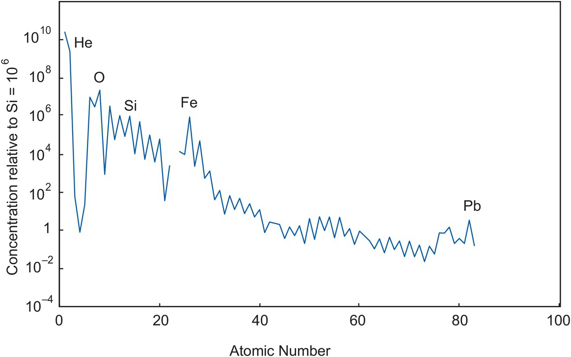
Figure 1.1 The abundances of elements in the sun, by atomic number, relative to the solar value Si = 10⁶.

(Data from Anders and Grevesse, 1989)

The chemical study of primitive meteorites illuminates our study of geochemistry in three important ways:

1. Knowing the chemical composition of the materials from which the Earth formed provides a geochemical baseline for measuring the differentiation of the Earth and the fractionation process that take place on the Earth. Typically, trace elements and isotopes are expressed relative to the chondritic composition of the Earth (Sections 4.3.2.2 and 6.2.2) as a measure of the original bulk Earth composition (BE). Alternatively, trace element abundances and isotope ratios may be expressed relative to the Earth’s primordial or primitive mantle (PM) which is the composition of the Earth after the separation of the core and represents the bulk silicate Earth (BSE) (see Sections 3.1.3, 4.4.1.2 and 6.2.2).
2. Some primitive meteorites contain information about processes in the solar nebula and more rarely about even earlier processes. Pre-solar grains of refractory minerals such as diamond and SiC can predate the solar nebula itself and stable isotope studies of elements such as Cr and Mn can provide information about the distribution of nucleosynthetic products in the early solar system (Section 7.4.4.3). Hydrogen isotope ratios are now available for a range of solar system objects and together with measurements made in meteorites are thought to indicate where in the solar system planets and other solar system objects formed (Section 7.3.2.2, Figure 7.7).
3. Meteorites also provide information about the large-scale differentiation of the Earth and the process of core formation. A knowledge of the mantle concentrations of those trace elements which have a high affinity for metallic iron, the highly siderophile elements (Section 4.5), coupled with experimental studies on their metal silicate partition coefficients (Table 4.10), provides information on the process of core formation. In a similar way, it is thought that carbon was sequestered into the Earth’s core, and so the mass balance of carbon isotopes in the Earth’s mantle also contributes to our understanding of this process (Section 7.3.3.2).

1.2.2 Processes Which Control the Chemical Composition of Igneous Rocks

The processes which control the composition of igneous rocks are summarised in Figure 1.2 and are illustrated for basaltic rocks.

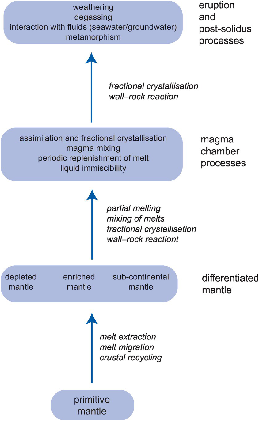
Figure 1.2 A flow diagram showing the main geochemical processes which operate during the genesis and eruption of basaltic rocks; the diagram is indicative of the geochemical processes which operate more generally in igneous rocks.

1.2.2.1 Processes Which Take Place in the Mantle Source

Basaltic rocks may be extracted by partial melting from a range of mantle source compositions the most primitive of which – the primitive mantle – is the product of the very early differentiation of the Earth. This process involved the separation of the core and maybe formed during the magma-ocean stage of early Earth history. Subsequent partial melting and mixing events have created the modern upper mantle which is differentiated into domains that are chemically depleted and enriched. Two main processes control the enrichment and depletion of the mantle. These are the extraction, migration and recrystallisation of partial melts, formed at different depths and representing different degrees of partial melting, and the recycling into the mantle of crustal materials through the process of subduction. Modern lavas derived from a source that has escaped later modification and so represents the Earth’s primitive mantle are extremely rare. One example is the 61 Ma picrites from Baffin Island in north-eastern Canada which represent a relatively high melt fraction of deep mantle and have a primitive isotopic signature (McCoy-West et al., Reference McCoy-West, Fitton, Pons, Inglis and Williams2018).

Characterising the chemical composition of a mantle source region and thereby understanding those processes which take place in the source region is best achieved by measuring its radiogenic isotope composition (Section 6.2) and using selected trace element ratios, sometimes known as canonical trace element ratios, because these ratios are not modified during partial melting and subsequent magma chamber processes (Section 4.6.1.3).

1.2.2.2 Partial Melting Processes

Unmodified melts produced by the partial melting of the mantle are known as primary magmas. Their chemical composition is controlled by two main factors. The first controls are those of the chemical composition of the source and its mineralogy. The composition of the source will reflect whether or not it is chemically enriched or depleted, and the mineralogy of the source is a measure of the depth of melting. The second set of controls are the physical conditions of melting, that is, the temperature and depth of melting, the precise mechanism of melting and the degree of partial melting (Section 4.2.2.2). In some instances, the oxygen fugacity of the mantle is also an important control. After the initial melting stage, the primary magma may be modified as it migrates through the mantle through mixing with melts from other sources and through crystallisation and wall–rock reaction processes. The major element, trace element and radiogenic isotope chemistry are all important in unravelling the origins of primary magmas.

1.2.2.3 Magma Chamber Processes

Most basaltic rocks are filtered through a magma chamber prior to their emplacement at or near the surface. These magma chambers may be located at the base of the crust or at various levels within the crust. They are fed by what is known as the parental magma, which may or may not be the same as a primary magma. A wide variety of magma chamber processes modify the chemical composition of the parental magma. These include fractional crystallisation, assimilation of the country rock and associated fractional crystallisation, the mixing of magmas from more than one source, the separation of melts through liquid immiscibility or a dynamic mixture of several of these processes (Sections 3.3.4.1, 4.2.2.3 and 6.3.5). Magma chambers are best thought of as dynamic systems into which melt is fed and is differentiated, in which cumulate rocks form and from which melt is erupted. Resolving the chemical effects of these different processes requires the full range of geochemical tools: major and trace element studies coupled with the measurement of both radiogenic and stable isotope compositions.

1.2.2.4 Post-solidus Processes

Following the emplacement or eruption of basaltic rocks they may be further chemically modified by the processes of outgassing or by interaction with a fluid such as seawater or groundwater. The outgassing or degassing of the dissolved gases in basaltic melts is the product of pressure release at the Earth’s surface, and the effects are often seen in their stable isotope geochemistry, for this process readily fractionates isotopes on the basis of mass differences (Section 7.3.4.2). Hydrothermal processes operate at a range of temperatures, from several hundred degrees where seawater or groundwater interact with a magma chamber to the much lower temperatures of chemical weathering. Depending upon the temperature, these processes will modify the mineralogy of the parent rock through the development of clay minerals, and both major and trace elements may be mobilised (Sections 3.1.2 and 4.2.2.1). This is seen in igneous plutonic bodies where on emplacement hydrothermal ground-water circulation in the surrounding country rocks is initiated leading to the chemical alteration of the igneous pluton itself and sometimes the formation of ore bodies through the enhanced concentration of elements which have been mobilised. In addition to using major and trace elements, hydrothermal activity can be monitored by the use of radiogenic and stable isotopes, particularly those of strontium, oxygen and hydrogen, to measure the extent of fluid–rock interaction (Sections 6.3.5.2 and 7.3.2.7).

1.2.3 Processes Which Control the Chemical Composition of Metamorphic Rocks

The principal control on the chemical composition of a metamorphic rock is the composition of the protolith, that is, the composition of the rock prior to its metamorphism. Metamorphism is frequently accompanied by deformation, and at high metamorphic grades there may be the mechanical mixing of different protolith compositions through tectonic interleaving, which can give rise to metamorphic rocks of mixed parentage.

Metamorphic recrystallisation is the result of chemical reactions which take place in the solid state by the process of diffusion. These reactions occur during the burial and heating of the protolith and during cooling. They may be isochemical, but most commonly there is a change in chemical composition. This chemical change is related to the mineralogical reactions which take place and the extent to which those elements found in the minerals in the protolith can be accommodated in the new minerals of the metamorphic rock. Most commonly, these mineralogical changes are also controlled by the movement of fluids in the rock. For this reason, the ingress and expulsion of water during metamorphism, chiefly as a consequence of metamorphic hydration and dehydration reactions, exerts the major control on element mobility during metamorphism. These processes are controlled by the composition of the fluid phase, most commonly H₂O and CO₂, its temperature and the ratio of the volume of metamorphic fluid to that of the host rock. The extent to which major and trace elements are mobile during metamorphism can sometimes be assessed by reference to the composition of the unmetamorphosed parent rock. Reactions between crustal fluids and metamorphic rocks and the relative volume of the fluids involved can be measured using the stable isotopes of hydrogen and oxygen (Section 7.3.2.7).

At high metamorphic grades, and frequently in the presence of a hydrous fluid, melting may occur. The segregation and removal of a melt phase will differentiate the parental rock into two compositionally distinct components: the melt and the unmelted component, known as the restite. In this case, the precise nature of the chemical change is governed by the melting reaction and the degree of melting (Section 3.4.3).

1.2.4 Low-Temperature Processes in the Earth’s Surficial Environment

Low-temperature processes in the Earth’s surficial environment include the wide array of interactions between the atmosphere, the hydrosphere, and rocks and soils at the Earth’s surface. These interactions are often summarised in diagrams representing geochemical cycles and can be represented by box models which show the mass balance for a particular element between the different Earth reservoirs. Examples of geochemical cycles quantified using stable isotope ratios are given in Chapter 7; see Figure 7.22 for the elements sulphur, carbon and oxygen, and Figure 7.27 for nitrogen. A cartoon diagram summarising the main surficial processes discussed here is given in Figure 1.3.

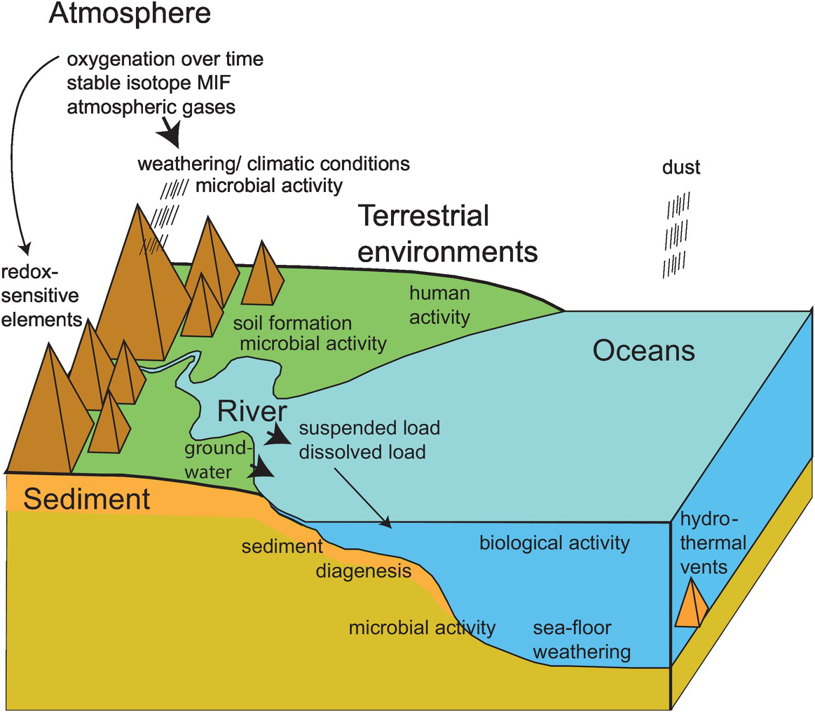
Figure 1.3 Cartoon diagram showing the interconnecting processes which operate at the Earth’s surface in the atmosphere, in terrestrial environments and in the oceans.

(Figure adapted from Frank et al., 2020. With permission from Elsevier)

1.2.4.1 Atmospheric Processes

A detailed discussion of geochemical processes occurring in the Earth’s atmosphere is beyond the scope of this book. However, there is one aspect of atmospheric geochemistry which is relevant to the petrological processes discussed here, for over geological time the chemical composition of the Earth’s atmosphere has become increasingly oxygenated. This change in the level of oxygen in the atmosphere has a direct bearing on the oxygenation of the oceans and on weathering processes. Thus, those elements which are redox sensitive at the Earth’s surface can play an important role in identifying the different levels of oxygenation in the oceans and other bodies of surface water. Particularly important are the redox sensitive trace elements (Section 4.2.1.3) and the stable isotopes of the transition metals, nitrogen and sulphur (Sections 7.4.4.3 and 7.4.5.3). The process of mass independent fractionation of sulphur isotopes plays a particularly important role in the detecting the earliest oxygenation of the Earth’s atmosphere (Section 7.3.4.4).

1.2.4.2 Weathering Processes

The interaction between the atmosphere and hydrosphere in the terrestrial environment leads to the development of a weathering profile and the formation of soils. This process is often biologically mediated and involves chemical reactions in which silicate minerals are converted into clays. These reactions are governed by the surface temperature and in some circumstances may be used to infer former climatic conditions. The intensity of chemical weathering has been quantified using the chemical index of alteration calculated from major element geochemistry (Section 3.3.1.5) and from the fractionation of the stable isotopes of lithium and silicon (Sections 7.4.1.3 and 7.4.3.2). The temperature of formation of the clay minerals kaolinite and smectite in the weathering environment has been estimated using hydrogen and oxygen isotopes (Section 7.3.2.4).

In the marine environment the interaction between seawater and the rocks of the ocean floor leads to the seafloor weathering of basalts. In some cases the isotopic composition of weathered ocean floor basalts is sufficiently different from that of unaltered basalt that this signature may be used to track the recycling of the altered basalts back into the Earth’s mantle. This is particularly pertinent for Li isotopes (Section 7.4.1.1) and Os isotopes (Section 6.3.3.4).

1.2.4.3 Water Chemistry

The chemical composition of river water is expressed in terms of its dissolved load and its suspended load of particulate matter. Different elements behave in different ways and some may be present in solution; others are adsorbed onto particulate matter. These two components are a consequence of the particular weathering environment, and because of this the chemical composition of rivers from across the globe is very variable. In some weathering environments the fractionation of stable isotopes during the formation of clay minerals is extreme and this geochemical signature can be transferred to river water and in the case of Li isotopes gives it a very distinctive isotopic composition (Section 7.4.1.3). In a similar way the stable isotopes of Mg, Si, Cr and Fe are also highly fractionated in river water relative to silicate rocks (Figures 7.32, 7.33, 7.35 and 7.36).

The chemical composition of seawater is influenced by the input of river water, groundwater, atmospheric dust, hydrothermal fluids, sea-floor weathering and biological activity (Figure 7.3). Ultimately, the elements present in seawater are taken up in to sediments, but the average length of time they remain in the seawater is highly variable. This time interval is known as the residence time. For a given element the length of the residence time is a measure of how well mixed the oceans are for that particular element. This is illustrated for the rare earth elements (REE) in Section 4.3.3.2 and radiogenic isotopes in Section 6.3.2.3. The geochemistry of the oceans is not the main focus of this book, although there are two themes which are of petrological interest. These are the interactions between seawater and the rocks of the ocean floor, and the way in which the composition of seawater has changed over time (Figure 6.13). Seawater–rock interactions have been monitored using the stable isotopes of hydrogen and oxygen (Section 7.3.2.7) and these have great relevance to the formation of mineral deposits. The changing composition of seawater can be evaluated in the changing isotopic composition of marine sediments such as those carbonates which are precipitated directly from seawater. The stable isotope ratios of carbon (Section 7.3.3.5) and lithium (Section 7.4.1.3) and the radiogenic isotope ratios of strontium and osmium (Section 6.3.2.3) are particularly sensitive.

1.2.4.4 The Impact of Human Activity on the Earth’s Surface Environment

The impact of anthropogenic activity is increasingly important in environmental geochemistry. Although beyond the scope of this book, two examples are pertinent. Recent work on nitrogen isotopes has shown that it is possible to fingerprint polluting anthropogenic nitrates (Section 7.3.5.3) and in a similar way the remediation of toxic Cr⁶⁺ in groundwater can be monitored using the stable isotopes of Cr (Section 7.4.4.3).

1.2.5 Processes Which Control the Chemical Composition of Sedimentary Rocks

1.2.5.1 Provenance

The geochemical make-up of the rocks constitutes the provenance which influences the composition of sediments. In immature sediments there is a direct geochemical link between the major and trace element composition of the sediment and its provenance (Section 5.5). The provenance of fine-grained, clay-rich sediments such as shale can be determined from selected trace elements and isotopes (Sections 4.2.2.4, 5.5.3 and 6.2.3.2). Provenance studies may also be used to determine the original tectonic setting of the basin in which fine-grained sediment formed (Section 5.5).

1.2.5.2 Weathering

Weathering conditions leave their signature in the resultant sediment and, as discussed above, major element and stable isotope studies of sedimentary rocks indicate that former weathering conditions can be recognised in the chemical composition of the sediments. Significant chemical changes may also take place during sediment transport, for some trace elements become concentrated in the clay fraction; others are concentrated in a heavy mineral fraction; while others are diluted in the presence of a quartz-rich fraction. To a large extent these processes are dependent upon the length of time the sediment spends between erosion and deposition.

1.2.5.3 Processes in the Depositional Environment

The chemical changes that occur during the deposition of sediments are governed by the nature of the depositional environment. This in turn is influenced by the subsidence rate and the attendant thermal conditions of the sedimentary basin. The temperature-dependent fractionation of oxygen isotopes can be used to calculate the geothermal gradient during diagenesis and allows some control on the burial history of the rock (Sections 7.2.5 and 7.3.1.2). In the case of chemical sediments the chemical and biochemical processes controlling the solubility of particular elements coupled with thermal and redox conditions are also important. Post-depositional, fluid-related diagenetic processes are best investigated using stable isotopes. The stable isotopes of oxygen and hydrogen are important tracers of different types of water (Section 7.3.2.3) and the combined application of carbon and oxygen isotopes are important in the study of limestone diagenesis (Section 7.3.3.9).

1.2.6 Biogeochemical Processes

Microbial life is abundant at the surface of the Earth and can leave a geochemical fingerprint in its stable isotope signature. This is because many microbially mediated chemical reactions cause mass fractionation in particular stable isotope systems. For example, the kinetics of the conversion of inorganic carbon into living carbon entails the preferential concentration of the light carbon isotope in the living carbon (Section 7.3.3.6). Isotopic signatures of this kind open up the possibility of identifying specific microbial reactions which may relate to particular metabolic pathways which may be found in both modern environments and in the ancient sedimentary record. Other examples of elements which are essential to life and whose stable isotopes are fractionated by microbial activity are sulphur and nitrogen. In the marine environment sulphur isotopes are fractionated during the reduction of seawater sulphate by anaerobic bacteria (Section 7.3.4.2) and nitrogen isotopes are fractionated during the reduction of nitrate to atmospheric nitrogen through the metabolic processes of denitrification and anammox (Section 7.3.5.2). Magnesium is also an essential element in the biosphere and there is evidence that Mg isotopes are fractionated in plants during photosynthesis (Section 7.4.2.3). Iron isotopes are fractionated during both anaerobic bacterial iron reduction and photosynthetic iron oxidation operating under anaerobic conditions (Section 7.4.5.2).

1.2.6.1 The Search for Early Life on Earth

The preservation of microbially driven stable isotope fractionations in the geological record has been used a means of identifying the presence of life on Earth from the earliest stages of Earth history. One of the first studies was by Schidlowski (Reference Schidlowski1988), who showed that the study of carbon isotopes can be used to trace ancient biological activity through the geological record back as far as 3.7 Ga (Section 7.3.3.7). Subsequent studies used the large negative sulphur isotope values in the sedimentary record as a means of exploring the processes of microbial sulphate reduction in the geological past (Section 7.3.4.6). It has also been suggested that the extreme iron isotope fractionations in Archaean sediments are, in part, the product of microbial activity, although as with other stable isotope systems it is important to establish whether or not similar fractionations could have been produced by abiotic processes (Section 7.4.5.3).

1.3 Geological Controls on Geochemical Data

The most fruitful geochemical investigations are those that test a particular model or hypothesis. This ultimately hinges upon a clear understanding of the geological relationships in the rock suite under investigation. Thus, any successful geochemical investigation must be based upon a proper understanding of the geology of the area. It is not sufficient to carry out a ‘smash and grab raid’, returning to the laboratory with large numbers of samples, if the relationships between the samples are unknown and their relationship to the regional geology is unclear. It is normal to use the geology to interpret the geochemistry. Rarely is the converse true, for at best the results are ambiguous.

In some instances this is self-evident, for example, when samples are collected from a specific stratigraphic sequence or lava pile or from drill core data, and there is a clear advantage in knowing how geochemical changes take place with stratigraphic height and therefore over time. A more complex example would be a metamorphosed migmatite terrain in which several generations of melt have been produced from a number of possible sources. A regional study in which samples are collected on a grid pattern may have a statistically accurate feel and yet will provide limited information on the processes in the migmatite complex. What is required in such a study is the mapping of the relative age relationships between the components present, at the appropriate scale, followed by the careful sampling of each domain. This then allows chemical variations within the melt and restite components to be investigated and models tested to establish the relationships between them.

A further consideration comes from the different scales on which geochemical data are collected. With the advent of microbeam analytical techniques and the continuation of programmes such as the ocean drilling or continental drilling programmes it is possible to measure geochemical data from the micro to macro scales. For example, the mapping of trace element or isotopic data in a single mineral grain may be used to illuminate processes such as fractionation in an igneous melt, diffusion in a metamorphic rock or changing fluid conditions during sediment diagenesis. This was illustrated in the study of the zonation of iron isotopes in olivines from Kīlauea Iki lava lake in Hawai‘i by Sio et al. (Reference Sio, Dauphas, Teng, Chaussidon, Helz and Roskosz2013). Equally, the mapping of isotopic variations in ocean floor basalts can be used to identify geographically specific compositional reservoirs in the Earth’s mantle. Hart (Reference Hart1984) mapped the southern hemisphere DUPAL anomaly in this way on the basis of anomalous Sr- and Pb-isotopic compositions. At an intermediate scale, the mapping of the distribution of Pb in stream sediments over a large area of eastern Greece has relevance for both environmental pollution and mineral exploration (see figure 2 in Demetriades, Reference Demetriades, Holland and Turekian2014).

A fundamental tenet of this book therefore is that if geochemical data are going to provide information about geological processes, then geochemical investigations must always be carried out in the light of a clear understanding of the geological relationships. This normally means that careful geological fieldwork is a prerequisite to a geochemical investigation. This approach leads naturally to the way in which geochemical data are presented. In the main this is as bivariate (and trivariate) plots in which the variables are the geochemical data. The interpretation of these plots forms the basis for understanding the geological processes operating.

1.3.1 Sample Collection

It is important that any new geochemical investigation has a well-developed sampling strategy. The key parameters are discussed in detail by Ramsay (Reference Ramsay and Gill1997) and for environmental applications by Demetriades (Reference Demetriades, Holland and Turekian2014). A brief summary is given here.

Sample size tends to be governed by the grain size of the rock. The overriding principle is that the sample must be representative of the rock. In addition, the portion of the sample used in geochemistry must be fresh and therefore an allowance must be made for any weathered material present which will be removed later. It is also important to retain part of the sample for future research and/or the preparation of a thin section.
Sampling will normally be done using a hammer. Occasionally, precise sampling or sampling from a difficult surface may be carried out using a coring drill. In either case care must be taken to establish that rock sampling is permitted at the site in question and that sampling is carried out as discretely as possible.
The number of samples is normally governed by the nature of the problem being solved. Relevant are the geographic extent of the study area and whether or not there are spatial or temporal aspects to the research project. If the research question is very specific a relatively small number (10–20) of well-chosen samples may suffice. Often many more samples than this are required. A further consideration is whether there is the opportunity to return to the field area. If not, then selecting a larger number of samples makes good sense.
The careful labelling of samples in the field, at the site of collection, is perhaps obvious. A geological description of the site is important, accompanied by photographs and the precise GPS location. This will allow the researcher or their successor to return to the precise sample site if necessary, and such information is often important in the future publication of the results.

1.4 Analytical Methods in Geochemistry

In this section the more widely used analytical methods are reviewed in order to provide a guide for those embarking on geochemical analysis. This text is not principally a book about analytical methods in geochemistry and excellent summaries are given by Gill (Reference Gill1997), Rouessac and Rouessac (Reference Rouessac and Rouessac2007) and in the second edition of volume 15 of the Treatise on Geochemistry (McDonough, Reference McDonough2014b). First, however, it is necessary to consider the criteria by which a particular analytical technique might be evaluated (Figure 1.4). In this book, in which geochemical data are used to infer geochemical processes, it is the quality of the data which is important. Data quality may be measured in terms of precision, accuracy and detection limits.

Figure 1.4 Obtaining geochemical data. A summary of the key issues to be considered when collecting geochemical data and in selecting an appropriate method of analysis.

Precision refers to the repeatability of a measurement. It is a measure of the reproducibility of the method and is determined by making replicate measurements on the same sample. The limiting factor on precision is the counting statistics of the measuring device used. Precision can be defined by the coefficient of variation which is 100 times the standard deviation divided by the mean (Till, Reference Till1974), also known as the relative standard deviation (Jarvis and Williams, Reference Jarvis and Williams1989). A common practice, however, is to equate precision with one standard deviation from the mean (Norman et al., Reference Norman, Leeman, Blanchard, Fitton and James1989). It can be helpful to distinguish between precision during a given analytical session (repeatability) and precision over a period of days or weeks (reproducibility).

Accuracy is about getting the right answer. It is an estimate of how close the measured value is to the true value. Knowing the true value can be very difficult, but it is normally done using recommended values for international geochemical reference standards (see Section 1.6.4). It is of course possible to obtain precise but inaccurate results.

The detection limit is the lowest concentration which can be ‘seen’ by a particular method and is a function of the level of background noise relative to the sample signal (Norish and Chappell, Reference Norrish, Chappell and Zussman1977). Where concentrations of a particular element are below the levels of detection for a particular analytical method, this is often reported in data tables as ‘bd’ (below the limits of detection; see Table 1.1).

1.4.1 Sample Preparation

In the laboratory, rock samples must be reduced to a fine powder for fusion or dissolution prior to geochemical analysis. This normally follows a number of stages. These include the splitting of the rock and the removal of any remaining weathered material; the crushing of the sample, often in a hardened steel jaw crusher; and then the pulverising of the sample to a fine powder in a ball mill or disc mill. Two key principles must be followed. First, the whole sample must be reduced to a powder and so the sample should not be sieved. Second, the chemical composition of the machinery used in the pulverisation of the rock sample must be chosen with the sample geochemistry in mind. It would be unwise to use a tungsten-carbide mill if tungsten is an element of interest because it is very probable that the sample will become contaminated with W during sample preparation.

1.4.2 Sample Dissolution

Many of the analytical methods describe below require the bulk rock sample to be in solution. Given the insoluble nature of silicate rocks this requires a number of acid dissolution, digestion and/or fusion techniques. It is essential that the entire rock, including resistant insoluble phases such as zircon or chromite, is completely dissolved and that the dissolution process is done in an ultra-clean environment so that the sample is not contaminated during the digestion process. A comprehensive review of the full range of dissolution techniques for analytical geochemistry is given by Hu and Qi (Reference Hu, Qi, Holland and Turekian2014). The main analytical methods currently in use in geochemistry are briefly described below.

1.4.3 X-Ray Fluorescence (XRF)

X-ray fluorescence spectrometry (XRF) was the work-horse of early-modern geochemistry and was widely used for the determination of major and trace element concentrations in rock samples. It is still widely used in mining geology and exploration geochemistry. The method is versatile: it can analyse up to 80 elements over a wide range of sensitivities detecting concentrations from 100% down to a few ppm and is rapid so that large numbers of precise analyses can be made in a relatively short space of time. Good reviews of the older applications of the XRF method are given by Leake et al. (Reference Leake, Hendry, Kemp, Plant, Harvey, Wilson, Coats, Aucott, Lunel and Howarth1969), Norrish and Chappell (Reference Norrish, Chappell and Zussman1977), Ahmedali (Reference Ahmedali1989) and Fitton (Reference Fitton and Gill1997) and there is a comprehensive recent review by Nakayama and Nakamura (Reference Nakayama, Nakamura, Holland and Turekian2014).

1.4.3.1 Wavelength Dispersive X-Ray Fluorescence Spectrometry (WDXRF)

X-ray fluorescence spectrometry is based upon the excitation of a sample by X-rays. A primary X-ray beam excites secondary X-rays (X-ray fluorescence) which have wavelengths characteristic of the elements present in the sample. The intensity of the secondary X-rays is proportional to the concentration of the element present and is used to determine the concentrations of the elements present by reference to calibration standards. In most XRF spectrometers the X-ray source is an X-ray tube in which the X-rays are generated by the bombardment of a target with electrons. For the analysis of geological samples, the target element, or anode of the X-ray tube, is Rh as the X-rays from Rh are capable of exciting a very wide range of elements. However, in some instances W, Au, Cr and Mo tubes may also be used. The intensity of the secondary X-rays is analysed in a wavelength dispersive spectrometer using either a gas proportional counter or a scintillation counter. In detail instruments vary in precisely how the analyses are made. In some a relatively small number of elements are measured simultaneously, in others a larger number of elements are measured sequentially.

1.4.3.2 Energy Dispersive X-Ray Fluorescence (EDXRF)

A more recent application of X-ray fluorescence technology is the development of energy dispersive X-ray fluorescence in which the X-ray energy is measured using a solid-state silicon drift detector (Potts et al., Reference Potts, Webb and Watson1990). This method allows the simultaneous measurement of a large number of elements and in principle can measure almost every element between Na to U at concentrations from a few ppm to nearly 100% within a few seconds. The detector identifies the radiation from the different elements present in the sample and analyses the energy on a multi-channel pulse height analyser.

The range of elements that may be detected during X-ray fluorescence analysis varies according to the type of instrument. In WDXRF the element range is from Be to U, whereas in EDXRF it is from Na to U. The limits of detection depend upon the element and the sample matrix, but generally the heavier elements have better detection limits. The better peak resolution of WDXRF means that there will be fewer spectral overlaps and the background noise is reduced so that detection limits and sensitivity are improved over EDXRF. In terms of speed of analysis and therefore cost, a spectrum is collected very rapidly in EDXRF, whereas with WDXRF the elements are analysed in sequence or in batches and therefore each analysis takes longer. Samples for trace element analysis are prepared as a pressed disc of the rock powder (Leake et al. Reference Leake, Hendry, Kemp, Plant, Harvey, Wilson, Coats, Aucott, Lunel and Howarth1969); for major element analysis a glass bead is made from a fusion of the powdered sample with a lithium metaborate or tetraborate flux.

New developments in XRF technology have led to the recent development of micro-XRF and portable XRF analysers. Micro-XRF uses the energy-dispersive method of detection and a narrow X-ray beam as an imaging tool to map microscopic particles and build high-resolution elemental maps of geological materials. Portable XRF analysers also use the energy-dispersive method of detection. They are capable of measuring a wide range of elements from Mg (some include Na) upwards in the periodic table and have detection limits of a few ppm to a few tens of ppm for trace elements of geological interest. Applications include the analysis of clean rock surfaces and drill core. Rowe et al. (Reference Rowe, Hughes and Robinson2012) discuss the application of portable XRF in the analysis of mudrocks.

1.4.4 Instrumental Neutron Activation Analysis (INAA)

Instrumental neutron activation analysis has been used in the past as a non-destructive technique for the determination of trace elements, particularly the REE. Instrumental neutron activation analysis (INAA) uses a about 100 mg of powdered rock or mineral sample; the sample is placed in a neutron flux in a neutron reactor and irradiated. The neutron flux gives rise to new, short-lived radioactive isotopes of the elements present which emit gamma radiation and are measured using a Ge detector (Hoffman, Reference Hoffman1992). Instrumental neutron activation analysis has now been superseded by more rapid and more accurate methods of trace element analysis and is no longer widely used.

1.4.5 Atomic Absorption Spectrophotometry (AAS)

Atomic absorption spectrophotometry (AAS) has been used in the past for major and trace element analysis. The method is based upon the observation that atoms of an element can absorb electromagnetic radiation when the element is atomised. A lowering of response in a detector during the atomisation of a sample in a beam of light as a consequence of atomic absorption can be calibrated and is sensitive at the ppm level (Price, Reference Price1972). However, this technique allows only one element to be analysed at a time, and so has been superseded by more rapid methods of silicate analysis and now is rarely used for geochemical analysis.

1.4.6 Mass Spectrometry

Mass spectrometry is an analytical technique which is particularly suited to the measurement of isotopes in geological samples (Figure 1.5). It offers very high precision, low levels of detection and may be applied to very small samples. Often, however, it requires extensive sample preparation which may involve the chemical separation of the element of interest. In this section we consider the techniques of thermal ionisation mass spectrometry (TIMS), gas source mass spectrometry and the isotopic method of isotope dilution mass spectrometry. In Section 1.4.7 we will consider inductively coupled plasma mass spectrometry (ICP-MS) and in Section 1.4.9 secondary ion mass spectrometry (SIMS). In each case, however, the principles are the same. All rely on the generation of a beam of charged ions which is fired along a curved tube through a powerful electromagnet in which the atoms are separated according to their mass in response to the forces operating in the magnetic field. A mass spectrum is produced in which the lighter ions are deflected with a smaller radius of curvature than heavy ions. The quantitative detection of the signal allows isotope ratios to be calculated. The main difference between these mass spectrometric techniques is the manner in which the sample is ionised.

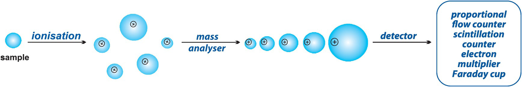
Figure 1.5 The essentials of mass spectrometry. The sample material is ionised and introduced into the mass spectrometer which is under vacuum. The ionised materials travel through the mass analyser, where ions are separated according to their charge to mass ratio, and then on to the detector where they are counted.

1.4.6.1 Thermal Ionisation Mass Spectrometry (TIMS)

In thermal ionisation mass spectrometry the sample is ionised on a glowing filament made of a high-melting-point metal, often Re. The method is particularly relevant to elements that have a high capacity for thermal ionisation and whose isotope systems are of interest. In geochemistry this includes Mg, Cr, Ti, Sr, Ba, Nd, Re, Os, W and Pb (Carlson, Reference Carlson, Holland and Turekian2014). Most elements of interest ionise as positive ions, but Re and Os are more efficiently ionised as negative ions. In his detailed review Carlson (Reference Carlson, Holland and Turekian2014) summarises the main strengths and weaknesses of the TIMS method. He shows that the main advantages of TIMS are the following: for those elements that ionise easily the ionisation is highly efficient; the molecular interference spectrum is quite simple; the thermal ionisation produces ions with a small energy spread allowing good mass resolution; and the potential for sample to sample cross contamination is small. Disadvantages are that for some elements of geological interest the ionisation efficiency is low and so the technique is unsuitable for Hf, W and positive Os ions; the chemical preparation of samples is complex and time-consuming; and corrections have to be made for the mass fractionation between isotopes during the process of thermal ionisation.

1.4.6.2 Gas Source Mass Spectrometry

Gas source mass spectrometry is used to measure the traditional stable isotopes (H, O, C, S and N) as described by Sharp (Reference Sharp, Holland and Turekian2014) and the noble gases (Wieler, Reference Wieler, Holland and Turekian2014). In stable isotope geochemistry rock samples are converted into a gas before the element of interest is introduced into the mass spectrometer: hydrogen as H₂, oxygen and carbon as CO₂, sulphur as SO₂ or SF₆ and nitrogen as N₂. The chemistry can be complex, as is the process of gas purification. The gas is introduced into the mass spectrometer using either a dual-inlet system or a continuous flow. In the dual-inlet system there is either the rapid switching between the sample and a standard reference gas or a dynamic inlet system in which the sample gas is constantly refreshed. In the continuous flow method a pulse of the sample gas is entrained in a helium stream, passed through a gas chromatographic column for purification, and into the mass spectrometer. The continuous flow method is popular, although there are isotope fractionations during the combustion of samples which must be accounted for in the data processing. Once in the mass spectrometer the sample gas is ionised by the impact of high-energy electrons from a tungsten filament.

1.4.6.3 Laser Fluorination Gas Source Mass Spectrometry

The in situ analysis of traditional stable isotopes (C, O, S, N) may be carried out using laser fluorination gas source mass spectrometry (Arevalo, Reference Arevalo, Holland and Turekian2014). This method has a very high spatial resolution for the analysis of mineral grains and permits the in situ analysis of individual micron-scale fluid and melt inclusions.

1.4.6.4 Isotope Dilution Mass Spectrometry

Isotope dilution mass spectrometry is the most accurate and most sensitive of all trace element analytical techniques and is particularly suited to measuring very low concentrations of trace elements to very high levels of accuracy and precision. The method is described in detail by Stracke et al. (Reference Stracke, Scherer, Reynolds, Holland and Turekian2014) and is applicable to the different mass spectrometric methods described above. Isotope dilution depends upon the addition of a known quantity of an element with a non-natural isotopic composition (known as a ‘spike’) to a known quantity of the sample. The isotopic composition of the spike–sample mixture is then measured by mass spectrometry, and from the known isotopic compositions of the sample and the spike it is possible to calculate the concentration of the element. The detail of the calculations is given in Stracke et al. (Reference Stracke, Scherer, Reynolds, Holland and Turekian2014). The method is applicable to any element which has two or more naturally occurring isotopes and has been particularly useful in geochronology and in determining the abundances of trace elements at very low concentrations. The main advantage of isotope dilution is that the method does not depend upon any external calibration, for element concentrations are determined directly from the masses of the sample and the spike and the measured isotopic compositions of the sample, spike and sample–spike mixture. Further, unlike other mass spectrometric methods isotope dilution does not depend upon the quantitative recovery of the element from the sample.

Double-spike isotope dilution methods require the addition of two spike isotopes and the analysis of four or more isotopes. This method uses two independently measured isotope ratios to determine two unknowns and is used to separate natural isotope fractionations from those induced by chemical processing or fractionations which occur during analytical measurements such as instrumental mass fractionation.

1.4.7 Inductively Coupled Plasma (ICP) Spectrometry

Inductively coupled plasma (ICP) spectrometry is an analytical method in which the sample is introduced into a plasma source in which the energy is supplied by electrical currents produced by electromagnetic induction. The inductively coupled plasma is a stream of argon atoms, heated by the inductive heating of a radio frequency coil and ignited by a high-frequency Tesla spark. The sample dissociates in the argon plasma into a range of atomic and ionic species. Samples are prepared in solution using the standard methods of silicate dissolution. There are two main applications of ICP spectrometry: the older technique of ICP-optical emission spectrometry and the more recently developed and now widely used technique of ICP-mass spectrometry.

1.4.7.1 ICP-Optical Emission Spectrometry (ICP-OES)

ICP optical emission spectrometry (ICP-OES), also known as ICP-atomic emission spectrometry (ICP-AES), is a light-source technique with a plasma temperature in the range 6000–10,000 K. A sample solution is passed as an aerosol from a nebuliser into an argon plasma. The sample dissociates in the argon plasma and a large number of atomic and ionic spectral lines are excited. Emission rays that correspond to photon wavelengths are measured and the element type and concentration is determined from the position and intensity of the photon rays, respectively. The spectral lines are detected by a range of photomultipliers; these are compared with calibration lines, and their intensities converted into concentrations. The ICP-OES method is capable of measuring most elements in the periodic table with low detection limits and good precision over several orders of magnitude. Elements are measured either simultaneously or sequentially. When measured simultaneously a complete analysis can be made in the space of about 2 minutes, making it an extremely rapid analytical method. A full description of the method and its application is given by Walsh and Howie (Reference Walsh and Howie1980) and Thompson and Walsh (Reference Thompson and Walsh1983).

1.4.7.2 ICP-Mass Spectrometry (ICP-MS)

ICP mass spectrometry is now widely used as a means of elemental and isotopic analysis, for the detection limits are extremely low and may be in the parts per trillion (ppt, ngl⁻¹) range. A review of the methodology and instrumentation is given by Olesik (Reference Olesik, Holland and Turekian2014). There are now a number of different types of mass spectrometer which are used in ICP analysis. These include the following:

Quadrupole mass spectrometers. Quadrupole instruments are widely used, for they are able to rapidly and sequentially measure the different atomic masses. However, it is necessary to use instrumental and/or mathematical corrections in the data processing to accommodate spectral overlaps.
Sector field mass spectrometers. These measure masses sequentially and can be used for isotope ratio measurements as well as elemental chemical analysis. They provide a much higher sensitivity or, alternatively, a much higher mass resolution than quadrupole instruments. Sector field mass spectrometers are more complex than quadrupole instruments and use a double focusing design to achieve the higher sensitivity or mass resolution. This means that ions with the same mass to charge ratio but different kinetic energies are focussed into a single location in the focal plane.
Multi-collector instruments (MC-ICP-MS). These use sector field mass spectrometry but with multiple detectors to measure isotopes simultaneously in order to determine isotope ratios with extremely high precision. However, multi-collector instruments require the chemical separation of the element of interest from the sample matrix.

1.4.7.3 Laser Ablation ICP Mass Spectrometry (LA-ICP-MS)

Laser ablation mass spectrometry is an in situ analytical method which can be used for measuring elemental concentrations down to very low abundances and radiogenic and non-traditional stable isotope ratios. The details of the methodology are given by Arevalo (Reference Arevalo, Holland and Turekian2014). The benefits of the LA-ICP-MS method are that it provides rapid, high-precision analysis, minimal sample processing and high spatial resolution of the data. The sample is ablated using either a pulsed Nd:YAG (Nd-doped yttrium aluminium garnet) laser system or an excimer laser system which employs gas mixtures of a noble gas and a halogen. The ablated material is then introduced into an ICP mass spectrometer. Issues of concern in the application of this technology are elemental fractionations which may take place during the ablation process or non-stoichiometric ablation. These may be accommodated using a range of operational protocols as outlined by Arevalo (Reference Arevalo, Holland and Turekian2014). The reduction in LA-ICP-MS data is carried out using a variety of software packages, and a recent study showed that different users can obtain significantly different results from the same raw data. For this reason, Branson et al. (Reference Branson, Fehrenbacher, Vetter, Sadekov, Eggins and Spero2019) recently proposed a new data-reduction package which provides some consistency in this field and allows for the reproducible reduction of LA-ICP-MS data.

1.4.8 Electron Probe Micro-analysis (EPMA)

Electron probe analysis is a microbeam technique which is principally used in the analysis of minerals and glasses. The method is reviewed by Reed (Reference Reed, Potts, Bowles, Reed and Cave1994). The sample is excited by a highly focused beam of electrons and X-rays are generated. The quantitative analysis of the sample is obtained by the analysis of the X-rays and as with X-ray fluorescence analysis these may be analysed in two ways. They may be analysed according to their wavelength or by their energy spectrum. In electron microprobe wavelength dispersive analysis, using a wavelength dispersive spectrometer (WDS), the X-rays are analysed in a series of element-specific detectors in which the peak area is counted relative to a standard, and intensities converted into concentrations after making appropriate corrections for the matrix (Long, Reference Long, Potts, Bowles, Reed and Cave1994). There are a variety of software packages which process the data. Energy-dispersive electron microprobe analysis, using an energy dispersive spectrometer (EDS), utilises an energy versus intensity spectrum and allows the simultaneous determination of the elements of interest. The spectrum is collected using a solid-state silicon drift detector. EDS analysis may also be made using a scanning electron microscope (SEM) with an attached solid-state detector and can be used for quantitative analysis provided it is calibrated with suitable standards. WDS is the more precise of the two methods and the speed of analysis is governed by the number of spectrometers on the instrument – often around 3 minutes for a ten-element analysis. EDS analysis prefers speed (about 1 minute to collect a spectrum) over very high levels of precision.

During the interaction between the electron beam and the sample secondary electrons and backscattered electrons are generated. These may be used, with the appropriate detectors, to provide an electron image of the sample and so guide the EPMA user to suitable ‘spots’ on the sample for analysis. Images may also be used for element mapping, in which the distribution pattern of a particular element is displayed within a mineral grain, and so is important in demonstrating features such as element zoning or exsolution.

The chief merit of the electron microprobe is that it has excellent spatial resolution and commonly employs an electron beam of 1–5 microns in diameter. This means that extremely small sample areas can be analysed and individual mineral grains can be analysed in great detail. Elements from B to U can be analysed, but most laboratories analyse only the major elements on a routine basis. Most geological applications are in the analysis of minerals and natural and synthetic glasses. The analysis of silicate glass is of particular importance in the analysis of tephra and the experimental charges in experimental petrology; less commonly fused discs of rock powder are analysed for major elements using this method (Staudigel and Bryan, Reference Staudigel and Bryan1981). In glass analysis a wider, defocussed electron beam is normally used to minimise the problems of sample volatilisation during analysis and inhomogeneity in the glass.

The development of field emission electron probe instruments (FE-EPMA), in which the microprobe is equipped with a thermal field emission gun electron source, has provided even better imaging and analytical resolution. FE-EPMA instruments can provide accurate quantitative analyses of individual grains as small as 300–400 nm and have the X-ray imaging capacity of down to 200 nm (Armstrong et al., Reference Armstrong, McSwiggen and Nielsen2013). Samples for EPMA are prepared for analysis by making a polished thin section of a rock slice or grain mount in epoxy resin. The polished surface is then sputter coated with a thin conductive layer of carbon or gold.

1.4.9 The Ion Microprobe (SIMS)

The ion microprobe, or ion-probe as it is also known, combines the analytical accuracy and precision of mass spectrometry with the very fine spatial resolution of the electron microprobe. It is widely used in the fields of geochronology, stable isotope geochemistry and trace element analysis. Reviews of the method and its application are given by Hinton (Reference Hinton, Potts, Bowles, Reed and Cave1994) and Ireland (Reference Ireland, Holland and Turekian2014). There are two principal instruments available, the SHRIMP (sensitive high-resolution ion microprobe) family of instruments from the Australian National University and Cameca instruments which include the NanoSIMS with nanometer resolution.

Ion microprobe technology employs a finely focussed beam of ions to bombard an area of the sample (typically 10–25 microns in diameter) and causes a fraction of the target area to be ionised and emitted as secondary ions. The ionisation process, known as sputtering, drills a small hole in the surface of the sample a few microns in depth. Samples are prepared as polished thin sections or grain mounts coated with carbon or gold. Before analysis, samples are normally characterised using conventional geological microscopy and electron imaging in order to determine the best sample area for analysis. Ion-probe analysis is non-destructive, highly sensitive and is capable of producing many analyses from a very small amount of material – important when multiple analytical methods on a single location are desired.

The primary ion beam is most commonly made up of either Cs or oxygen ions. Cs⁺ is used for non-metals such as O or S, and oxygen for metals such as Pb⁺. There is a trade-off during analysis between spatial resolution and precision – the larger the spot size, the larger the mass sputtered which typically results in better precision, but at the cost of spatial resolution. The spectrum of the secondary ions is analysed using a sector mass spectrometer to determine the isotopic composition of the sample – hence the term ‘secondary ion mass spectrometry’ (SIMS).

Ion probe analysis is used in both trace element and isotopic analysis. It can be used in the determination of the abundance of volatile species H, O, S, N, C, F and Cl and the analysis of traditional and non-traditional stable isotopes. It is often used in geochronology and applied to the U-Th-Pb and Hf isotope systems. A particular application is the U-Pb geochronology of zircon grains, for these contain measurable quantities of U and Th but not Pb. Ion probe analysis may also be used in exploring diffusion profiles in minerals through the sequential sputtering of a grain during depth profiling.

The development of nanoSIMS allows a much finer spatial resolution than conventional SIMS instruments and operates with spot sizes as low as 50 nm for a caesium beam and 200 nm for an oxygen beam (Ireland, Reference Ireland, Holland and Turekian2014). Zhang et al. (Reference Zhang, Lin, Yang, Shen, Hao, Hu and Cao2014) measured sulphur isotopes at the submicron scale in pyrite and sphalerite using a ∼0.7 pA Cs⁺ beam of ∼100 nm diameter and scanning over areas of 0.5 × 0.5 μm². They documented external reproducibility (1 SD) of better than 1.5‰ for both δ³³S and δ³⁴S.

1.4.10 Synchrotron X-Ray Spectroscopic Analysis

A synchrotron is a charged particle accelerator which generates intense radiation. Of interest here is the application of synchrotron radiation in the X-ray part of the spectrum to geochemical analysis. One such microbeam method is X-ray absorption fine structure (XAFS) spectroscopy. This method can provide a detailed picture of the average electronic and molecular energy levels associated with multivalent elements, and allows the determination of valence state, coordination number and nearest neighbour bond lengths (Sutton and Newville, Reference Sutton, Newville, Holland and Turekian2014). An important application of XAFS spectra to geochemistry is the X-ray absorption near-edge structure (XANES) energy region. The micro-version of this application (μ-XANES) spectroscopy has been used to determine in situ the Fe³⁺/ΣFe ratio in basaltic glasses. The detail of the methodology is given in Kelley and Cottrell (Reference Kelley and Cottrell2009).

1.5 Selecting an Appropriate Analytical Technique

Choosing an analytical technique in geochemistry depends entirely upon the nature of the problem to be solved with the ultimate goal of understanding the processes that have taken place in a given suite of rocks. In part this requires selecting the right samples in the field. For example, consider a suite of basaltic lavas derived from a mantle source. In their journey to the surface the magmas will have experienced a wide range of fractionation and mixing processes which will have modified the composition of the original primitive mantle melt. In order to characterise the composition of the original melt this sequence of interactions must be progressively removed. A helpful way of doing this is to follow the flow diagram in Figure 1.2 backwards. This means at the sample selection stage those samples that show any evidence of fluid interaction during weathering, hydrothermal alteration or metamorphism are eliminated from the sample set. The remaining samples are examined using major and trace element geochemistry to identify magma chamber processes and the composition of the primary melt which fed the magma chamber. This then allows the identification of what is normally a small suite of the least fractionated and least contaminated samples which might be primary magmas and can be used reflect processes operating in the mantle source region. These samples can be further investigated using trace element and isotope geochemistry in order to understand the processes operating in the source region.

A similar sequence of sample selection may be followed for a suite of granitic rocks, although in this case identifying the nature of the source – crust or mantle – may be more complex. Further, the solidified rock may be a crystal-laden melt, and so it is sometimes necessary to identify those samples which represent true melt compositions. Further, the distribution of some trace elements may be governed by the presence of minor phases such as monazite, which is rich in P and the light REE, and phases of this type must be identified using petrography. It may also be important to know the age of the granite, in which case the isotopic analysis of its zircon is a commonly used technique. The oxygen and Hf isotope composition of the zircon may also provide further constraints on the composition and age of the source.

The choice of analytical technique also depends upon the nature of the material to be investigated. For example, a sample that is already in solution such as seawater or river water is amenable to analysis by ICP methods – ICP-OES or ICP-MS – immediately after dilution or pre-concentration. On the other hand, a rock sample crushed to a powder can be analysed by XRF after being made into a pressed powder pellet or fused into a glass disc; otherwise, it has to be turned into a solution using a ranging of fluxing and acid treatments. Once in solution it is then amenable to analysis by ICP methods – ICP-OES or ICP-MS. If samples are to be analysed by TIMS or INAA, then analysis must be preceded by sample digestion and the chemical separation of the element(s) of interest. The stable isotope analysis of a rock powder using gas source mass spectrometry requires that the sample is converted to a gas and undergoes sample purification for the element of interest. The non-destructive analysis of solid samples can be carried out using in situ methods such as the electron microprobe for major element and some trace element analysis, and the ion microprobe or laser ablation ICP-MS for trace elements and isotopes. These methods require a relatively small amount of sample preparation and can also function with very small samples.

Further considerations are the number of samples to be analysed and so the amount of sample preparation time involved, the speed of chemical analysis, the cost of the analysis and the precision required. In general terms XRF and ICP-OES and ICP-MS methods are rapid and can cope with large numbers of samples at relatively low cost, although both methods require the rock to be in powder form and so there is a certain amount of sample preparation involved. Other isotope methods – TIMS, isotope dilution mass spectrometry and gas source mass spectrometry – involve much greater sample preparation but isotope dilution offers the best possible precision. In some cases it is possible to screen a large number of samples using techniques such as quadrupole ICP-MS or in the case of in situ analysis LA-ICP-MS and then carry out high-precision analysis of a selected number of samples using either much longer counting times or very precise methods such as SIMS or isotope dilution.

1.6 Sources of Error in Geochemical Analysis

Normally, if samples are collected carefully and if sample preparation is carried out in a clean environment following conventional analytical protocols, the geochemical data are safe to use. However, there are a number of ways in which the results of geochemical analysis can be in error and it is important for the user to be alert to these possibilities. They are briefly reviewed below.

1.6.1 Contamination

The user of geochemical data must always be alert to the possibility that samples have become contaminated. This is known to have happened in sometimes the most bizarre circumstances such as when petrol spilt on rock samples in a boat resulted in spurious Pb isotope analyses, or the more avoidable convergence of Pb isotope compositions of a suite of igneous rocks with that of Indian Ocean seawater, when the samples were collected from a beach on the Indian Ocean.

More subtle is the contamination which may take place during sample preparation. This can occur during crushing and grinding and may arise either as cross-contamination from previously prepared samples or from the grinding apparatus itself. Cross-contamination can be eliminated by careful cleaning and by pre-contaminating the apparatus with the sample to be crushed or ground. For the highest precision analyses samples should be ground in agate, although this is delicate and expensive and even agate may introduce occasional contamination (Jochum et al., Reference Jochum, Seufert and Thirlwall1990). Tungsten carbide, a commonly used grinding material in either a shatter box or a ring mill, can introduce sizeable tungsten contamination, significant Co, Ta and Sc and trace levels of Nb (Nisbet et al., Reference Nisbet, Deitrich and Esenwein1979; Hickson and Juras, Reference Hickson and Juras1986; Norman et al., Reference Norman, Leeman, Blanchard, Fitton and James1989; Jochum et al., Reference Jochum, Seufert and Thirlwall1990). Chrome steel introduces sizeable amounts of Cr, Fe, moderate amounts of Mn and trace amounts of Dy and high carbon steel significant Fe, Cr, Cu, Mn, Zn and a trace of Ni (Hickson and Juras, Reference Hickson and Juras1986).

Other sources of laboratory contamination may occur during sample digestion and arise from impure reagents or from the laboratory vessels themselves. This therefore requires ultra-clean laboratory procedures and the use of ultra-pure chemicals. A measurement of the level of contamination from this source can be made by analysing the reagents themselves in the dilutions used in sample preparation and determining the composition of the ‘blank’.

Natural contamination of samples may occur through the processes of weathering or through contact with natural waters. This may be remedied by removing all weathered material from the sample during sample slitting and leaching the rock chips with 1 M HCl for a few minutes after splitting but before powdering.

1.6.2 Calibration

Most of the methods of analysis described above measure concentrations relative to international standards of known composition or to a calibration curve derived therefrom. Calibration curves are drawn on the basis of standards of known composition and are used to convert counts per second in the instrument to ppm or wt.% in the sample. Standards used in the construction of calibration curves are either ultra-pure chemical reagents or international reference samples, as well as so-called in-house standards. Where matrix effects are important, such as with LA-ICPMS, standards should be of similar composition to the unknowns being investigated. Clearly, the accuracy of the final analysis of the unknown depends upon the accurate analysis of the standards used in calibration. It is possible for systematic errors to be introduced and these can be minimized if standard samples are interspersed and analysed as unknowns throughout the analytical session.

1.6.3 Peak Overlap

In most geochemical analytical techniques there is little attempt to separate the element to be analysed from the rest of the rock or mineral sample. Given that current analytical methods are generally a form of spectrometry, there is the possibility of interference between spectral lines or mass peaks so that the value measured is spuriously high due to overlap from a subsidiary peak of another element present in the rock. The effects of these interferences must be calculated and removed mathematically and in some cases minimised in the design of the instrument.

1.6.4 Detecting Errors in Geochemical Data

Errors in one’s own data can be detected by routinely running well-analysed in-house or international standards as unknowns through the sample preparation and analytical system. This will alert the user to calibration errors. It is also important to know about potential peak overlaps for elements of particular interest. Errors may be detected if samples have anomalous compositions. In this case the hand specimen and thin section of the sample should be investigated carefully to determine the reason for the anomalous nature of the sample and whether or not it has a real geological explanation, or whether it is an artefact of the analytical process. Anomalously low concentrations of certain elements relative to those expected for a particular rock type might reflect the incomplete dissolution of the sample during sample preparation.

Errors are minimised by using international reference materials and certified reference materials. These are essential for instrument calibration, method validation and quality control, and form the basis of interlaboratory comparisons. A thorough review of reference materials in geochemical and environmental research is given by Jochum and Enzweiler (Reference Jochum, Enzweiler, Holland and Turekian2014) and up-to-date information can be obtained from the GeoReM database at http://georem.mpch-mainz.gwdg.de/ and in the academic journal Geostandards and Geoanalytical Research.

Book contents

1 - Geochemical Data

Summary

Keywords