


1. Introduction
Supervised ensemble learning—sometimes referred to as a mixture of experts, classifier ensembles, or multiple classifier system (Saleh et al., Reference Saleh, Farsi and Zahiri2016; Milliken et al., Reference Milliken, Bi, Galway and Hawe2016) is a paradigm within the machine learning area concerned with integrating multiple base supervised learners in order to produce better predictive models than simply learning a single strong model. An ensemble typically performs its predictions by using a voting mechanism (e.g., majority voting) that computes the mean or the mode of the predictions output by the ensemble’s members (base learners). Ensemble learning methods have won several academic and industrial machine learning competitions (Sagi & Rokach, Reference Sagi and Rokach2018), and such methods have been extensively deployed in real-world AI applications (Oza & Tumer, Reference Oza and Tumer2008; Tabassum & Ahmed, Reference Tabassum and Ahmed2016).
Ensembles have several advantages over a single learner: (i) it is usually computationally cheaper to integrate a set of simple, weak models than to induce a single robust, complex model (Krithikaa & Mallipeddi, Reference Krithikaa and Mallipeddi2016); (ii) ensembles composed by classifiers that are, in turn, only slightly better than random guessing, can still present predictive performance comparable to a strong single classifier (Freund & Schapire, Reference Freund and Schapire1995; Liu et al., Reference Liu, Li, Zhang and Du2009; Jackowski et al., Reference Jackowski, Krawczyk and Woźniak2014); (iii) different base learners can be specialized in different regions of the input space, making their consensus more flexible and effective when dealing with complex problems (Freund & Schapire, Reference Freund and Schapire1995). Indeed, there is both theoretical and empirical evidence demonstrating that a good ensemble can be obtained by combining individual models that make distinct errors (e.g., errors on different parts of the input space) (Kim & Cho, Reference Kim and Cho2008a; Hansen & Salamon, Reference Hansen and Salamon1990; Krogh & Vedelsby, Reference Krogh and Vedelsby1995; Opitz & Maclin, Reference Opitz and Maclin1999; Hashem, Reference Hashem1997).
Ensemble learning comprises three distinct stages, whose names vary in the literature: generation, selection, and integration (Castro & Von Zuben, Reference Castro and Von Zuben2011; Britto et al., Reference Britto, Sabourin and Oliveira2014; Lima & Ludermir, Reference Lima and Ludermir2015), which is the most common naming system, and the one that will be used in this paper; pre-gate, ensemble-member, and post-gate (Debie et al., Reference Debie, Shafi, Merrick and Lokan2016); or generation, pruning, and fusion (Parhizkar & Abadi, Reference Parhizkar and Abadi2015a). The three-step generation of ensembles can be reduced to a hypothesis-search problem in combinatorial spaces, and so it is often approached by a variety of heuristic approaches, such as boosting (Freund & Schapire, Reference Freund and Schapire1995), bagging (Breiman, Reference Breiman1996), and Evolutionary Algorithms (EAs) (Lima & Ludermir, Reference Lima and Ludermir2015; Lacy et al., Reference Lacy, Lones and Smith2015b).
EAs have several advantages for ensemble learning, such as: performing a global search, which is less likely to get trapped into local optima than greedy search methods (Xavier-Júnior et al., Reference Xavier-Júnior, Freitas, Feitosa-Neto and Ludermir2018); being easily adapted for multi-objective optimization (Deb, Reference Deb2011); and dealing with multiple solutions in parallel, due to their population-based nature, for example Hauschild and Pelikan (Reference Hauschild and Pelikan2011), Kumar et al. (Reference Kumar, Husian, Upreti and Gupta2010). Hence, many EAs for supervised ensemble learning have been proposed in the literature in the past few years.
Several application domains have benefited from EA-based ensemble learning algorithms, including for example wind speed prediction (Woon & Kramer, Reference Woon and Kramer2016; Zhang et al., Reference Zhang, Qu, Zhang, Mao, Ma and Fan2017a), cancer detection (Krawczyk et al., Reference Krawczyk, Schaefer and Woźniak2013; Krawczyk & Woźniak, Reference Krawczyk and Woźniak2014; Krawczyk & Schaefer, Reference Krawczyk and Schaefer2014; Krawczyk et al., Reference Krawczyk, Schaefer and Woźniak2015, Reference Krawczyk, Galar, Jeleń and Herrera2016; Singh et al., Reference Singh, Sanwal and Praveen2016), noise bypass detection in vehicles (Redel-Macías et al., Reference Redel-Macías, Navarro, rrez, Cubero-Atienza and Hervás-Martínez2013), stock market prediction (Chen et al., Reference Chen, Yang and Abraham2007; Mabu et al., Reference Mabu, Obayashi and Kuremoto2014, Reference Mabu, Obayashi and Kuremoto2015), and microarray data classification (Park & Cho, Reference Park and Cho2003b, 2003a; Kim & Cho, Reference Kim and Cho2005, Reference Kim and Cho2008a; Liu et al., Reference Liu, Huang and Zhang2007, Reference Liu, Tong, Xie and Zeng2014a, 2015; Chen & Zhao, Reference Chen and Zhao2008; Rapakoulia et al., Reference Rapakoulia, Theofilatos, Kleftogiannis, Likothanasis, Tsakalidis and Mavroudi2014; Kim & Cho, Reference Kim and Cho2015; Ali & Majid, Reference Ali and Majid2015; Saha et al., Reference Saha, Mitra and Yadav2016), to name just a few.
This paper presents a survey of EAs for supervised ensemble learning. Our main contribution is to properly identify, categorize, and evaluate the available research studies in this area. This survey is aimed toward researchers on evolutionary algorithms and/or ensemble learning algorithms.
As related work, several surveys have been published on ensemble studies from different perspectives. Regarding specifically EAs for supervised ensemble learning, Yao and Islam (Reference Yao and Islam2008) present a review of EAs for designing ensembles, but they focus only on artificial neural networks (ANNs) as the base learners to be combined. Sagi and Rokach (Reference Sagi and Rokach2018), as well as Dietterich (Reference Dietterich2000) present a general review of ensemble learning studies, based on traditional non-evolutionary methods. Rokach (Reference Rokach2010), Kotsiantis (Reference Kotsiantis2014), and Tabassum and Ahmed (Reference Tabassum and Ahmed2016) review ensembles designed only for classification tasks. Similarly, Mendes-Moreira et al. (Reference Mendes-Moreira, Soares, Jorge and de Sousa2012) and Vega-Pons and Ruiz-Shulcloper (Reference Vega-Pons and Ruiz-Shulcloper2011) review ensemble methods for regression and clustering tasks only, respectively. There are also papers on specific domain applications of ensembles, for example Athar et al. (Reference Athar, Butt, Anwar and Latif2017), which reviews ensemble methods for sentiment analysis; Gomes et al. (Reference Gomes, Barddal, Enembreck and Bifet2017) and Krawczyk et al. (Reference Krawczyk, Minku, Gama, Stefanowski and niak2017) also review ensemble learning for data stream classification and regression.
Despite the relevant contributions of the previously cited literature, this work is to the best of our knowledge the first review to focus on general-application EAs for supervised ensemble learning in a comprehensive fashion. In particular, we highlight the following contributions: (i) we provide a general overview of EAs for supervised ensemble learning, not exclusively focusing on any specific EA or any given type of supervised model, but presenting an in-depth analysis of the different algorithms proposed for each stage of ensemble learning, with their respective advantages and pitfalls; and (ii) we provide a detailed taxonomy to properly categorize supervised evolutionary ensembles, helping the reader to filter the literature and understand the possibilities when designing EAs for this task. Note that reviewing EAs for ensemble learning in unsupervised settings (e.g., the clustering task) is out of the scope of this paper.
The rest of this paper is organized as follows. Section 2 briefly reviews the most well-known types of ensemble learning methods. Section 3 presents our novel taxonomy to categorize EAs designed for supervised ensemble learning. Sections 4, 5, and 6 review the EAs employed for the three stages of ensemble learning: generation, selection, and integration. In the next sections, we focus on broader aspects of EAs for ensemble learning that are not specific to any single stage, as follows. Section 7 details types of fitness functions often used by EAs for ensemble learning. Section 8 summarizes the types of EAs used for ensemble learning. Section 9 points to the most common base learners within the EAs reviewed in this survey. Section 10 describes the complexity of evolutionary algorithms when applied to ensemble learning. Finally, in Section 11 we summarize our findings by identifying patterns in the frequency of use of different methods across the surveyed EAs, and identify future trends and interesting research directions in this area.
2. Ensemble learning
There are three main motivations to combine multiple learners (Dietterich, Reference Dietterich2000): representational, statistical, and computational. The representational motivation is that combining multiple base learners may provide better predictive performance than a single strong learner. For example, the generalization ability of a neural network can be improved by using it as base learner within an ensemble (Chen & Yao, Reference Chen and Yao2006). In theory, no base learner will have the best predictive performance for all problems, as stated by the No Free Lunch theorem (Wolpert & Macready, Reference Wolpert and Macready1997); and in practice, selecting the best learner for any given dataset is a very difficult problem (Fatima et al., Reference Fatima, Fahim, Lee and Lee2013; Kordík et al., Reference Kordík, Černý and Frýda2018), which can be addressed by integrating several good learners into an ensemble.
The statistical motivation is to avoid poor performance by averaging the outputs of many base learners. While averaging the output of multiple base learners may not produce the overall best output, it is also unlikely that it will produce the worst possible output (Hernández et al., Reference Hernández, Hernández, Cardoso and Jiménez2015). This is particularly the case for data with few data points, so overfitting is more likely.
Finally, the computational motivation is that some algorithms require several runs with distinct initializations in order to avoid falling into bad local minima. Gradient descent, for example, often requires several runs and further evaluation on a validation set in order to avoid being trapped into local minima. Thus, it seems reasonable to integrate these already-trained intermediate models into an ensemble, stabilizing and improving the system’s overall performance (Tsakonas & Gabrys, Reference Tsakonas and Gabrys2013; de Lima & Ludermir, Reference de Lima and Ludermir2014).
Ensemble learning became popular during the 1990’s (de Lima & Ludermir, Reference de Lima and Ludermir2014), with some of the most important work arising around that time: stacking in 1992 (Wolpert, Reference Wolpert1992); boosting in 1995 and 1996 (Freund & Schapire, Reference Freund and Schapire1995, Reference Freund and Schapire1996; Schapire, Reference Schapire1999); bagging in 1996 (Breiman, Reference Breiman1996); and random forests in the early 2000’s (Breiman, Reference Breiman2001). We call these methods traditional to differentiate them from EA-based ensembles, though they are also referred to as preprocessing-based ensemble methods in the EA literature (Krawczyk et al., Reference Krawczyk, Galar, Jeleń and Herrera2016). We briefly review them next.
2.1 Boosting
Boosting refers to the technique of continuously enhancing the predictive performance of a weak learner (Krawczyk et al., Reference Krawczyk, Galar, Jeleń and Herrera2016). We present here the popular AdaBoost algorithm, proposed by Freund and Schapire (Reference Freund and Schapire1995). Given a set of predictive attributes
 $\mathbf{X}$
and a set of class labels
$\mathbf{X}$
and a set of class labels
 $Y, y \in Y = \{-1, +1\}$
, in its first iteration AdaBoost assigns equal importance (weights) to each instance in the training set,
$Y, y \in Y = \{-1, +1\}$
, in its first iteration AdaBoost assigns equal importance (weights) to each instance in the training set,
 $D_1(i) = 1/N$
,
$D_1(i) = 1/N$
,
 $i = 1, \dots, N$
, with N as the number of instances. For a given number of iterations G, AdaBoost trains a weak classifier based on the distribution
$i = 1, \dots, N$
, with N as the number of instances. For a given number of iterations G, AdaBoost trains a weak classifier based on the distribution
 $D_{g}$
and then computes its error
$D_{g}$
and then computes its error
 $\epsilon_g = \text{P}_{i \sim D_g} [h_g{(x_i)} \neq y_i]$
. Instances that are harder to classify will have their weights increased, so it becomes more rewarding to the model to classify them correctly.
$\epsilon_g = \text{P}_{i \sim D_g} [h_g{(x_i)} \neq y_i]$
. Instances that are harder to classify will have their weights increased, so it becomes more rewarding to the model to classify them correctly.
Candidate algorithms for boosting must support assignment of weights for instances. If this is not possible, a set of instances can be sampled from
 $D_g$
and supplied to the
$D_g$
and supplied to the
 $g{\rm th}$
learner. Although boosting usually improves the predictive performance of a weak classifier, its performance suffers when faced with noisy instances, since failing to correctly classify those instances will iteratively improve their importance and hence lead the learner to overfitting (Lacy et al., Reference Lacy, Lones and Smith2015b).
$g{\rm th}$
learner. Although boosting usually improves the predictive performance of a weak classifier, its performance suffers when faced with noisy instances, since failing to correctly classify those instances will iteratively improve their importance and hence lead the learner to overfitting (Lacy et al., Reference Lacy, Lones and Smith2015b).
2.2 Bagging
Bootstrap aggregating, or simply bagging, aims at reducing training instability when a learner is faced with a given data distribution (Breiman, Reference Breiman1996). It consists of generating B subsets of size N from the original training distribution
 $D(i) = 1/N$
,
$D(i) = 1/N$
,
 $i = 1, \dots, N$
with replacement, causing some instances to be present in more than one subset. As a result, some base learners have a tendency to favor such instances, having more opportunities to correctly predict their values. The predictions of all trained B learners are combined by computing their mean (regression task) or mode (classification task).
$i = 1, \dots, N$
with replacement, causing some instances to be present in more than one subset. As a result, some base learners have a tendency to favor such instances, having more opportunities to correctly predict their values. The predictions of all trained B learners are combined by computing their mean (regression task) or mode (classification task).
By sampling different subsets of instances for different classifiers, bagging implicitly injects diversity within the ensemble (Lacy et al., Reference Lacy, Lones and Smith2015b), whereas boosting explicitly does this by weighting the data distribution to focus the base learners’ attention into more difficult instances (Gu & Jin, Reference Gu and Jin2014; Lacy et al., Reference Lacy, Lones and Smith2015b).
2.3 Stacking
Compared to bagging and boosting, stacked generalization or simply stacking (Wolpert, Reference Wolpert1992) is a more flexible strategy for ensemble learning. The user can choose one or more types of base learners to be used in the ensemble (e.g., using only decision trees, or mixing them with ANNs Shunmugapriya & Kanmani, Reference Shunmugapriya and Kanmani2013). Then, each base learner will output a prediction, and all learners’ predictions will be combined by a meta-learner (which can also be chosen) to produce a single output. Popular traditional meta-learners for stacking include linear regression (for regression) and logistic regression (for classification). In Section 6.1 we review evolutionary algorithms used for learning logistic regression and linear regression algorithms’ weights. Stacking often improves the overall predictive performance of ensembles, making it a popular method (Shunmugapriya & Kanmani, Reference Shunmugapriya and Kanmani2013; Milliken et al., Reference Milliken, Bi, Galway and Hawe2016).
2.4 Random forests
Random forests, proposed by Breiman (Reference Breiman2001), is a type of ensemble learning method where both the base learner and data sampling are predetermined: decision trees and random sampling of both instances and attributes. The training process for the original random forests algorithm (Breiman, Reference Breiman2001) is described as follows. First, the algorithm randomly samples with replacement B subsets of training instances, one for building each of B decision trees that will compose the ensemble. For each inner node within a decision tree, the algorithm first randomly samples without replacement a subset of m attributes, and then it selects, among those attributes, the one that minimizes the local class impurity for that node. In this context, purity is the ratio of instances from difference classes that follow the same tree branch; hence, maximum purity in a node means that all instances reaching said node belong to the same class. This procedure is applied to each inner node in the current decision tree within the ensemble, and it is repeated until the tree achieves maximum class purity for all leaf nodes.
Random forests sometimes perform better than boosting methods, while being resilient to outliers and noise, faster to train than bagging and boosting methods (depending on the respective base learner), and being easily parallelized. However, it can require very many decision trees to provide an acceptable predictive performance, depending on the dataset at hand. Table 1 presents a brief overview of the main characteristics of the above traditional methods.
Table 1. Traditional ensemble learning methods compared. Adapted from Ma et al. (Reference Ma, Fujita, Zhai and Wang2015)

3. Ensemble learning with evolutionary algorithms
In general, Evolutionary Algorithms (EAs) are robust optimization methods that perform a global search in the space of candidate solutions. EAs are simple to implement, requiring little domain knowledge and can produce several good solutions to the same problem due to their population-based nature (Galea et al., Reference Galea, Shen and Levine2004). In particular, EAs seem to be naturally suited for ensemble learning, given their capability of producing a set of solutions that can be readily integrated into an ensemble (Duell et al., Reference Duell, Fermin and Yao2006; Lacy et al., Reference Lacy, Lones and Smith2015b). EAs also support multi-objective optimization (based e.g., on Pareto dominance), allowing the generation of solutions that cover distinct aspects of the input space (Lacy et al., Reference Lacy, Lones and Smith2015b) and removing the need to manually optimize some hyper-parameters (e.g., the base learner’s hyper-parameters, the number of ensemble members, etc.). However, EAs will likely increase the computational cost of ensemble learning, due to its robust global-search behavior that usually considers many tens or hundreds of possible solutions at each iteration (generation). Nonetheless, parallelization is an option to mitigate such problem (Lima & Ludermir, Reference Lima and Ludermir2015).
Since ensemble learning is composed of at least three main optimization steps (generation, selection, and integration), each one with many tasks, there is plenty of room to employ EAs (Fernández et al., Reference Fernández, Cruz-Ramrez and Hervás-Martnez2016b). In the literature on EA-based ensembles for supervised learning, the most common approach is to optimize a single step, though some studies go as far as optimizing two of them (e.g., Chen & Zhao, Reference Chen and Zhao2008; Ojha et al., Reference Ojha, Abraham and Snášel2017). Figure 1 summarizes how many studies were dedicated to each of the three stages.

Figure 1. Work summarized by the ensemble learning stage that EAs are employed. While generation is more popular than selection and integration combined, none of the surveyed studies employed EAs in all stages.
In this work, we provide a taxonomy to categorize the EA-based approaches for supervised ensemble learning (Figure 2). All surveyed studies are focused on supervised problems, that is, no unsupervised approach is reviewed.
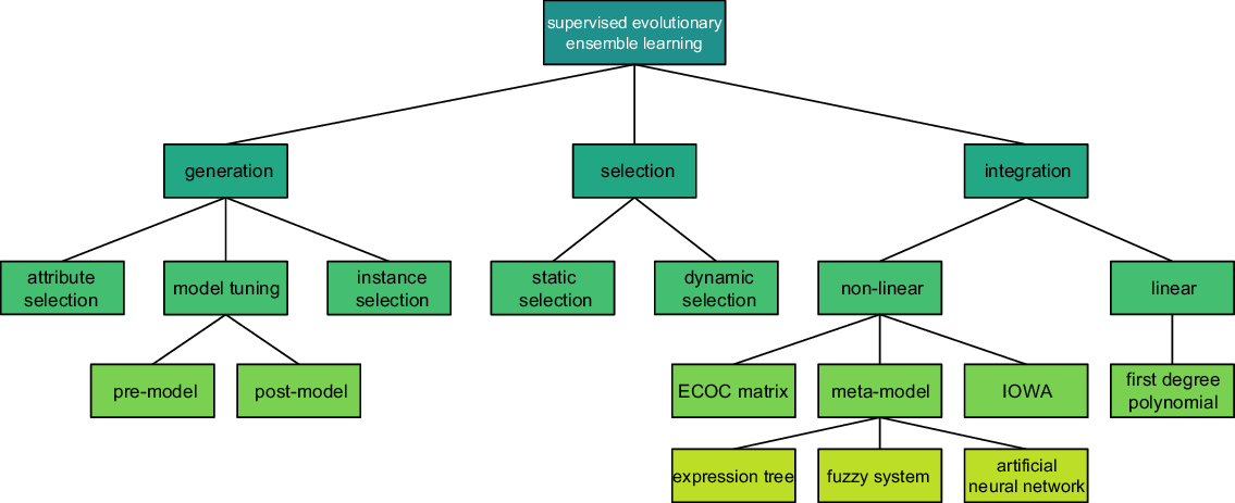
Figure 2. The proposed taxonomy for EAs employed in ensemble learning.
We divide the surveyed studies according to the well-established main stages of supervised ensemble learning: generation, selection, and integration. We use these three stages at the top level of our proposed taxonomy because in principle major decisions about the design of the EA (e.g., which individual representation to use, which fitness function to use) are entirely dependent on the type of ensemble learning stage addressed by the EA. The approaches most often used in each stage are presented at the second level of the taxonomy. For example, attribute selection, model tuning, and instance selection are the three most common approaches for the generation stage. Further divisions in the taxonomy are presented at the next levels, whenever it is the case.
Note that taxonomies vary depending on the aspect being analyzed—for example Gu (Gu & Jin, Reference Gu and Jin2014) is concerned with the generation stage and hence proposes a taxonomy exclusively for that step. To the best of our knowledge, our taxonomy is one of the broadest with regard to EAs for ensemble learning, with the closest reference being the one proposed by Cruz et al. (Reference Cruz, Sabourin and Cavalcanti2018). While the description of generation and selection stages in Cruz et al. (Reference Cruz, Sabourin and Cavalcanti2018) is identical to ours, we are more specific regarding the strategies for the integration stage. In addition, while the authors propose a two-level taxonomy, we present a more detailed and thorough four-level taxonomy.
3.1 Methodology to collect and analyze papers in this survey
The main objective of this work is to identify and evaluate existing approaches that apply evolutionary algorithms for learning ensembles of predictive models for supervised machine learning. The objective is expressed from the research questions presented in Table 2. These questions aim to analyze the relevant work, both in the context of evolutionary algorithms used, and the characteristics of ensembles that are optimized. The sections where these questions are addressed are also shown in the table.
3.1.1 Search strategy
Based on the main objective, we select keywords that are likely to be present in most of the work that proposes evolutionary algorithms for ensemble learning; from these keywords we compose a search string. Synonyms of each term were incorporated using the Boolean operator OR, whereas the Boolean operator AND was used to link the terms. The generic search string derived is
‘ensemble’ AND
(‘classification’ OR ‘classifier’ OR ‘classifiers’) OR
(‘regression’ OR ‘regressor’ OR ‘regressors’) AND
(‘evolutionary’ OR ‘evolution’)
In addition to the search string, we define the search engines. Thus, reviewed papers of this survey were searched in the following repositories: ScopusFootnote 1, Science DirectFootnote 2, IEEE XploreFootnote 3, and ACM Digital LibraryFootnote 4. Figure 3 shows the search strings as used in each search engine.
Table 2. Research questions of this survey
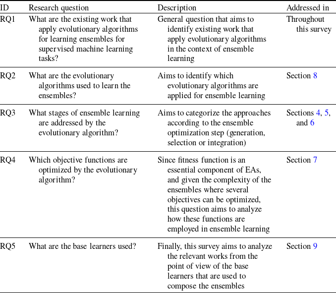

Figure 3. Search strings as used in search engines.
3.1.2 Study selection criteria
We adopted the following criteria for including studies in this survey: (i) papers that present a new evolutionary strategy for ensemble learning in supervised machine learning; (ii) papers that present a minimum detail of the proposed solution, including: type of EA used, fitness function used, ensemble stage optimized, base learners used; and (iii) papers that present an experimental evaluation of the proposed solution. We also use exclusion criteria, which are: (i) unavailability: paper not available in any online repository, or papers available only under payment; (ii) wrong topic: on further review, papers that did not cover the surveyed topic; and (iii) papers that are not written in English.
3.1.3 Study selection procedures
In the selection process, the search string was applied to the title, abstract, and keywords of searched papers. Scopus was the first repository searched, since it has the largest database. Eight hundred and two (802) papers matched the keywords. All papers had their abstracts reviewed, and from their analysis the ones deemed relevant (366) were carried on to the next stage of the reviewing process, as shown in column Relevant of Table 3.
We proceed the search with ACM Digital Library, IEEE Xplore, and Science Direct, again reviewing abstracts and selecting papers based on their relevance to this survey. Since Scopus is the largest database, some papers present in the remaining repositories were also present in Scopus. For this reason, column Already in Scopus of Table 3 counts the number of papers found in other repositories that already had their abstracts reviewed when we collected papers from Scopus. Among the remaining databases, we found 108 unique papers, not present in Scopus; from these, 38 were deemed relevant for further review.
Across all searched databases, 404 papers were deemed relevant for the survey, taking into consideration the description of their abstracts. From these, 50 were unavailable, either because (i) the document was not found in their host websites, or it was behind a paywall; or (ii) on further review of the paper, the topic addressed was not exactly the one we were interested (43 papers), as discussed in the beginning of Section 3.1.2. This reduced the number of relevant papers to 311.
From the remaining 311 papers, 164 were fully reviewed and included in the survey, with the remaining 147 not included nor reviewed. While we could have reviewed the latter group, we did not because we applied a truncation factor: that is, the rate at which we were detecting new concepts in papers was not justified by the amount of papers needed to reach these novel ideas. The papers that were not reviewed did not have any characteristic that made them less attractive than the ones reviewed, and we do not discriminate based on vehicle of publication, type of publication (conference or journal paper), date, number of citations, etc. An overall summary of the papers is presented in Figure 4.
Table 3. Papers that matched the search strings shown in Figure 3. In this stage all papers had their abstracts reviewed. From this initial analysis, not all papers were deemed relevant to the scope of this survey. Already in Scopus column denote papers that were already present at the Scopus database


Figure 4. From the 404 papers selected for review, 164 were added to the survey. Among these, 20 were duplicated (e.g., expanded work), and 144 original work.
Papers were reviewed in chronological order: the ones closest to the date of the reviewing process were added first, and the ones that had been already been published, reviewed last. From the papers that made to the survey, 20 were duplicated and fell into one of the following categories: (i) the algorithms were published in conferences and had expanded versions in journals; (ii) they had different application domains, but the algorithm was the same; or (iii) slightly different implementations (for example, changing the number of layers and/or activations in a neural network).
3.1.4 Data extraction strategy
After selecting the 164 works to compose the survey, the extraction and analysis of the data was made through peer review, where at least two researchers evaluated each work. The data were structured in a spreadsheet according to its meta-data (catalog information) and the characteristics of the work, according to the research questions that we aimed to answer.
We make available two supplementary material to this paper. The first is a repository of source code, hosted at https://github.com/henryzord/eael, with metadata used to generate figures and tables in this paper. The other is a master table, made available as a website, and hosted at https://henryzord.github.io/eael, listing individual information on surveyed work.
4. The generation stage of ensemble learning
In this stage the algorithm generates a pool of trained models. Those models may come from: (i) different paradigms (e.g., Naïve Bayes, support vector machines (SVMs), and Neural Networks Peimankar et al., Reference Peimankar, Weddell, Jalal and Lapthorn2017); or (ii) be from the same paradigm, but still present some differences, such as ANNs with different topologies and/or activation functions (Zhang et al., Reference Zhang, Qu, Zhang, Mao, Ma and Fan2017a).
The main objective in this stage is to generate a pool of both accurate and diverse base learners. Base learners must be diverse in order to provide source material for the selection and integration steps to work with. A diverse pool of base learners has more chances to commit errors in different data instances, thus correctly predicting more instances (Pagano et al., Reference Pagano, Granger, Sabourin and Gorodnichy2012).
An example of an ensemble algorithm that focuses on the generation phase is random forests (Breiman, Reference Breiman2001; Trawiński et al., Reference Trawiński, Cordón, Quirin and Sánchez2013), considering that it selects distinct subsets of both attributes and instances for building different decision trees, resulting in an ensemble of trees that is more robust than a single decision tree.
We have identified three ways of generating pools of learners that are both diverse and accurate: (i) providing distinct training sets for each base learner (instance selection); (ii) providing the same training set for all learners but with distinct sets of attributes (attribute selection); and (iii) optimizing the model by modifying the hyper-parameters and/or the structure of the base learners.
4.1 Instance selection
Instance selection, also known as prototype selection or data randomization (Vluymans et al., Reference Vluymans, Triguero, Cornelis and Saeys2016; Albukhanajer et al., Reference Albukhanajer, Jin and Briffa2017) consists of providing different (not necessarily disjoint) subsets of training instances for different base learners (Almeida and Galvão, Reference Almeida and Galvão2016; Rosales-Pérez et al., Reference Rosales-Pérez, a, Gonzalez, Coello and Herrera2017). This approach is well suited for homogeneous sets of base learners which are sensitive to changes in the instance distribution (e.g., decision trees Hernández et al., Reference Hernández, Hernández, Cardoso and Jiménez2015).
Instance selection can also be used to reduce training time by finding a subset of representative instances for each class (Almeida & Galvão, Reference Almeida and Galvão2016; Rosales-Pérez et al., Reference Rosales-Pérez, a, Gonzalez, Coello and Herrera2017). This is also beneficial for problems with high class imbalance, given that re-sampling instances with replacement makes it possible to simulate a uniform distribution among classes. Indeed that is one of the capabilities of the traditional bagging algorithm (Breiman, Reference Breiman1996). Thus, ‘bagged’ EAs are likely to have the same benefits as ‘bagged’: improved noise tolerance and reduced overfitting risk (Vluymans et al., Reference Vluymans, Triguero, Cornelis and Saeys2016). A method for selecting instances is needed since random sampling can lead to information loss and poor model generalization (Karakatič et al., Reference Karakatič, Heričko and Podgorelec2015). By using an EA, both the tasks of undersampling the majority class and oversampling the minority class are possible in parallel.
This section mainly focuses on instance selection techniques, since instance generation is more scarce. While the former performs a selection of instances from the original data, the latter can create new artificial instances, thus easing the adjustment of decision boundaries of models, at the expense of being more prone to overfitting (Vluymans et al., Reference Vluymans, Triguero, Cornelis and Saeys2016). Only one work uses a hybrid selection-and-generation strategy, namely (Vluymans et al., Reference Vluymans, Triguero, Cornelis and Saeys2016). In this work, seeking to address the class imbalance problem, a Steady State Memetic Algorithm (SSMA) is used for selecting instances from the training set, composing several individuals (i.e., subsets of instances). Once the SSMA optimization ends, a portion of its (fittest) individuals will be then fed to a Scale Factor Local Search in Differential Evolution (SFLSDE), that will improve the quality of instance subsets by generating new instances. Both evolutionary algorithms use a measure of predictive performance as the fitness function. Finally, the (fittest) individuals from SFLSDE are used by 1-NN classifiers, integrated by means of weighted voting (not evolutionary induced).
Although instance selection is present in work tackling the class imbalance problem (e.g., Cao et al., Reference Cao, Li, Zhao and Zaiane2013a; Galar et al., Reference Galar, Fernández, Barrenechea and Herrera2013; Vluymans et al., Reference Vluymans, Triguero, Cornelis and Saeys2016), it can lead to overfitting, or having subsets where one class has many more instances than other classes, if an inadequate objective function (such as accuracy) is used. An approach to avoid overfitting is to assign different misclassification costs to different classes. Typical cost-sensitive learning techniques do not directly modify the data distribution, but rather take misclassification costs into account during model construction (Cao et al., Reference Cao, Li, Zhao and Zaiane2013a).
Instance selection can be divided into wrapper and filter methods. In our literature review, wrapper methods were more common than filter methods. Only the work of Almeida and Galvão (Reference Almeida and Galvão2016) uses a filter approach, where a GA is used to optimize the number of groups in a k-means algorithm. Due to the tendency of k-means in finding hyperspherical clusters, the objective is to find evenly distributed groups of instances. One classifier is trained for each group, and the quality of classifiers is assessed by the weighted combination of training accuracy, validation accuracy, and distribution of classes within groups. In the prediction phase, unknown instances will be assigned to their most similar cluster, based on the Euclidean distance between the unknown-class test instance and the cluster’s instances.
For wrapper methods, usually the set of selected instances is encoded as either a binary or real-valued chromosome of N positions (the number of instances). In the binary case, each bit encodes whether an instance is present or absent in the solution encoded by the current individual. In a real-valued case, each gene encodes the probability that the respective instance will be present in that solution. To address class imbalance, in Galar et al. (Reference Galar, Fernández, Barrenechea and Herrera2013) only majority class instances are encoded in a binary string—minority class instances are always selected.
It is also possible to perform instance selection together with other methods. In Rosales-Pérez et al. (Reference Rosales-Pérez, a, Gonzalez, Coello and Herrera2017), the multi-objective problem consists in optimizing both a SVM’s hyper-parameters and the instance set to be used for training each model. This combined strategy is better for SVMs than simply selecting training subsets, since SVMs are robust to small changes in data distribution (Batista et al., Reference Batista, Rodrigues and Varejão2017). Coupling two tasks at once also fits well with weight optimization: in Krawczyk et al. (Reference Krawczyk, Galar, Jeleń and Herrera2016), evolutionary undersampling and boosting are used in a C4.5 decision tree classifier to iteratively optimize its performance in grading breast cancer malignancy.
Olvera-López provides an extensive survey of both evolutionary and non-evolutionary instance-selection methods proposed until 2010 (Olvera-López et al., Reference Olvera-López, Carrasco-Ochoa, Martnez-Trinidad and Kittler2010).
4.2 Attribute selection
Attribute selection, also called feature selection or variable subset selection (Sikdar et al., Reference Sikdar, Ekbal and Saha2012), offers distinct subsets of attributes to different base learners in order to induce diversity among base models. By removing irrelevant and redundant attributes from the data, attribute selection can improve the performance of base learners (Sikdar et al., Reference Sikdar, Ekbal and Saha2014b). Reducing the number of attributes also reduces the complexity of learned base models and may improve the efficiency of the ensemble system.
Attribute selection also performs dimensionality reduction and is an efficient approach to build ensembles of base learners (Liu et al., Reference Liu, Li, Zhang and Du2009). There is no need to provide disjoint sets of attributes to different learners. The base learners must be sensitive to modifications in the data distribution. SVMs, for example, were reported to be little affected by attribute selection (Vaiciukynas et al., Reference Vaiciukynas, Verikas, Gelzinis, Bacauskiene, Kons, Satt and Hoory2014).
Wrapper methods are by far the most common type of EAs for attribute selection. It has been noted that there is a direct link between high-quality attribute subsets and a high-quality pool of base learners (Mehdiyev et al., Reference Mehdiyev, Krumeich, Werth and Loos2015). Filter approaches break this link, evaluating the quality of an attribute set in a way independent from the overall base learner pool (Mehdiyev et al., Reference Mehdiyev, Krumeich, Werth and Loos2015).
A wrapper method provides a reduced subset of attributes to a learning algorithm, and then the predictive accuracy of the model trained with those attributes is used as a measure of the quality of the selected attributes. The random subspace method, for example, is a traditional approach for wrapping algorithms that randomly selects different attribute subsets for different base learners. Although this method is usually much faster than EAs, its performance is sensitive to the number of attributes and ensemble size (Liu et al., Reference Liu, Li, Zhang and Du2009). By contrast, EAs can improve stability and provide more accurate ensembles (Liu et al., Reference Liu, Li, Zhang and Du2009). Other examples of traditional methods include sequential forward selection, sequential backward selection, beam search, etc. (Mehdiyev et al., Reference Mehdiyev, Krumeich, Werth and Loos2015).
However, filter methods are still usually preferred for some application domains, such as microarray data, where the number of attributes far surpasses the number of instances, rendering a wrapper approach inefficient. In Kim and Cho (Reference Kim and Cho2008a), base learners are coupled with filters that perform attribute selection. Although the authors do not use training time as an objective in the EA, the reported execution time of a single run of the GA is between 15 seconds to 3 minutes, much faster than an exhaustive search, that could take as long as one hour (for sets of 24 attributes), or one year (for sets of 42 attributes), in a dataset of 4026 attributes. Their proposed algorithm is also capable of outperforming other EA-based ensembles for two microarray datasets. In another study, genetic algorithms (GAs) with error rate as fitness function were shown to be capable of outperforming greedy wrapper methods in terms of ensemble accuracy (Mehdiyev et al., Reference Mehdiyev, Krumeich, Werth and Loos2015).
Two concepts relevant for attribute selection are sparsity and algorithmic stability. An attribute selection algorithm is called sparse if it finds the sparsest or nearly sparsest set of attributes subject to performance constraints (e.g., small generalization error) (Vaiciukynas et al., Reference Vaiciukynas, Verikas, Gelzinis, Bacauskiene, Kons, Satt and Hoory2014). An algorithm is called stable if it produces similar outputs when fed with similar inputs—that is, it selects similar attribute sets for two similar datasets (Xu et al., Reference Xu, Caramanis and Mannor2012). As noted in Vaiciukynas et al. (Reference Vaiciukynas, Verikas, Gelzinis, Bacauskiene, Kons, Satt and Hoory2014), Xu et al. (Reference Xu, Caramanis and Mannor2012), stability and sparsity constitute a trade-off. An algorithm that is sparse may be incapable of selecting similar sets of attributes across runs (Vaiciukynas et al., Reference Vaiciukynas, Verikas, Gelzinis, Bacauskiene, Kons, Satt and Hoory2014).
EAs for attribute selection vary on the number of objectives to be optimized, integration with other stages, and distribution of base learners. In Peimankar et al. (Reference Peimankar, Weddell, Jalal and Lapthorn2016, Reference Peimankar, Weddell, Jalal and Lapthorn2017) a multi-objective Particle Swarm Optimization algorithm provided different attribute subsets to heterogeneous base learners, in order to predict whether power transforms will fail in the near future. In Sikdar et al. (Reference Sikdar, Ekbal and Saha2016, Reference Sikdar, Ekbal and Saha2014b, 2015), two Pareto-based multi-objective differential evolution algorithms performs attribute selection, and then linear voting weight optimization, in a pipeline fashion (the generation stage is performed before the integration stage).
The encoding used in Kim et al. (Reference Kim, Street and Menczer2002) considers each individual as an ensemble of classifiers. Classifiers are trained differently based on their input features. Each classifier competes with its neighbors within the same ensemble; and at a higher level, ensembles compete among themselves based on their predictive accuracy.
4.3 Model optimization
Models may have their hyper-parameters and/or structure modified while creating a pool or ensemble of base learners. We divide this category of our taxonomy into two groups: pre-model and post-model optimization.
Pre-model optimization involves fine-tuning the hyper-parameters of the base learners that will generate the base models. We call these approaches pre-model because the optimization happens prior to model generation. Examples are: tuning a neural network’s learning rate; a SVM’s type of kernel function (Rosales-Pérez et al., Reference Rosales-Pérez, a, Gonzalez, Coello and Herrera2017); L2 regularization (Woon & Kramer, Reference Woon and Kramer2016); and random forests’ number of trees (Saha et al., Reference Saha, Mitra and Yadav2016).
Pre-model approaches may support heterogeneous sets of base learners. For example, in Saha et al. (Reference Saha, Mitra and Yadav2016) the authors select both the types of base learner and their respective hyper-parameters, together with a set of attributes that will be assigned to a given learner. They used the NSGA-II (Deb et al., Reference Deb, Pratap, Agarwal and Meyarivan2002) algorithm, and the one-point crossover keeps base models and hyper-parameters together, only allowing to swap the selected attributes for each model.
Post-model approaches try to improve an existing model. Examples are layout and inner node selection for decision trees (Augusto et al., Reference Augusto, Barbosa and Ebecken2010; Wen & Ting, Reference Wen and Ting2016; Mauša & Grbac, Reference Mauša and Grbac2017), and topology, weight, and activation function optimization in neural networks (Fernández et al., Reference Fernández, Cruz-Ramrez and Hervás-Martnez2016b; Ojha et al., Reference Ojha, Abraham and Snášel2017). Weights are also optimized in Krithikaa and Mallipeddi (Reference Krithikaa and Mallipeddi2016), where an ensemble of heterogeneous parametric models are optimized by differential evolution.
Post-model encoding depends on the type of base learner being used, and so are more common on homogeneous sets of base learners. In Kim and Cho (Reference Kim and Cho2008b), the weights of ANNs are modified by a GA. The authors adopt a matrix of size
 $W \times W$
, where W is the number of neurons in the entire network. The upper diagonal encodes whether two given neurons are connected, and the lower diagonal encodes the weights associated with those connections.
$W \times W$
, where W is the number of neurons in the entire network. The upper diagonal encodes whether two given neurons are connected, and the lower diagonal encodes the weights associated with those connections.
Some studies perform both pre- and post-model optimization. In Ojha et al. (Reference Ojha, Abraham and Snášel2017), first the topology of a neural network is evolved by using NSGA-II. The best found topology then has its parameters (e.g., weights and activation functions) adjusted by a multi-objective Differential Evolution method. In the end, the final population is submitted to a voting scheme optimized by another EA.
Attribute selection is often coupled with model optimization. In Tian and Feng (Reference Tian and Feng2014), both post-model optimization of Radial Basis Function Neural Networks and attribute selection were used, by performing both approaches in two subpopulations of the Cooperative Coevolutionary EA. In Rapakoulia et al. (Reference Rapakoulia, Theofilatos, Kleftogiannis, Likothanasis, Tsakalidis and Mavroudi2014), solutions for both tasks were placed within the same chromosome: in a 132-wide chromosome array, 88 bits are designated for attribute selection, 10 bits represent parameter nu and threshold (integer and decimal part), 14 bits correspond to the gamma value and 20 bits are used for the parameter C of a nu-SVR learner.
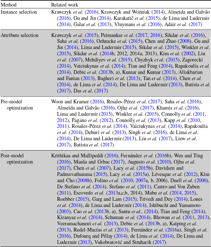
Table 4 summarizes the work on EAs for the generation step of supervised ensemble learning, based on the taxonomy proposed in this section.
Table 4. Categorization of studies that employ EAs in the generation stage of supervised ensemble learning
5. The selection stage of ensemble learning
From the pool of generated base models, model selection (or model pruning Parhizkar & Abadi, Reference Parhizkar and Abadi2015a) is performed in order to define the final set of base models for the ensemble. Selection may be regarded as a multi-objective problem, where two objectives—predictive performance, and diversity—must be optimized. When the size of an ensemble is large, selecting base models based on these metrics can be computationally expensive if all ensemble options are considered, thus making the use of meta-heuristics (such as evolutionary algorithms) attractive (Parhizkar & Abadi, Reference Parhizkar and Abadi2015a). However, simpler options (such as simply selecting the
 $\Phi$
most accurate learners) can also be used. Selection is often viewed as an optional stage and frequently not performed by traditional methods (e.g., boosting Freund & Schapire, Reference Freund and Schapire1995, bagging Breiman, Reference Breiman1996) or EA-based ones (e.g., Cao et al., Reference Cao, Zhao and Zaiane2013b; Zagorecki, Reference Zagorecki2014).
$\Phi$
most accurate learners) can also be used. Selection is often viewed as an optional stage and frequently not performed by traditional methods (e.g., boosting Freund & Schapire, Reference Freund and Schapire1995, bagging Breiman, Reference Breiman1996) or EA-based ones (e.g., Cao et al., Reference Cao, Zhao and Zaiane2013b; Zagorecki, Reference Zagorecki2014).
Whether or not to perform selection is an issue for debate, with some authors proposing to bypass this stage (i.e., using the entire pool of models as ensemble) (Trawiński et al., Reference Trawiński, Cordón and Quirin2014). Lacy et al. (Reference Lacy, Lones and Smith2015b) argue that model selection is irrelevant for ensemble learning, and that it is sufficient to select the
 $\Phi$
best models from the pool. According to Lacy et al. (Reference Lacy, Lones and Smith2015b), Freund and Schapire (Reference Freund and Schapire1996), Cagnini et al. (Reference Cagnini, Basgalupp and Barros2018), from a predictive performance standpoint, this approach would be more effective than building an ensemble while considering diversity metrics. Other authors claim that there is little correlation between ensemble diversity and accuracy (Opitz, Reference Opitz1999; Breiman, Reference Breiman2001; Parhizkar & Abadi, Reference Parhizkar and Abadi2015a; Cagnini et al., Reference Cagnini, Basgalupp and Barros2018). On the other hand, some authors argue the opposite: for example, for regression, Wang and Alhamdoosh (Reference Wang and Alhamdoosh2013) argue that the
$\Phi$
best models from the pool. According to Lacy et al. (Reference Lacy, Lones and Smith2015b), Freund and Schapire (Reference Freund and Schapire1996), Cagnini et al. (Reference Cagnini, Basgalupp and Barros2018), from a predictive performance standpoint, this approach would be more effective than building an ensemble while considering diversity metrics. Other authors claim that there is little correlation between ensemble diversity and accuracy (Opitz, Reference Opitz1999; Breiman, Reference Breiman2001; Parhizkar & Abadi, Reference Parhizkar and Abadi2015a; Cagnini et al., Reference Cagnini, Basgalupp and Barros2018). On the other hand, some authors argue the opposite: for example, for regression, Wang and Alhamdoosh (Reference Wang and Alhamdoosh2013) argue that the
 $\Phi$
best neural networks may not produce an ensemble with better mean squared error (MSE). This is also stated by Liu et al. (Reference Liu, Tong, Xie and Yee Ng2015), adding that simply selecting the most accurate models may result in loss of predictive performance given that most of those models may be strongly correlated, leaving the opinion of the minority of the committee underrepresented.
$\Phi$
best neural networks may not produce an ensemble with better mean squared error (MSE). This is also stated by Liu et al. (Reference Liu, Tong, Xie and Yee Ng2015), adding that simply selecting the most accurate models may result in loss of predictive performance given that most of those models may be strongly correlated, leaving the opinion of the minority of the committee underrepresented.
Although Lacy et al. (Reference Lacy, Lones and Smith2015b) and Liu et al. (Reference Liu, Tong, Xie and Yee Ng2015) have different opinions on the utility of model selection, both agree that diversity measures are not a good proxy for ensemble quality, with Liu et al. (Reference Liu, Tong, Xie and Yee Ng2015) suggesting that accuracy on a validationFootnote 5 set is sufficient. The rationale for using diversity measures is that by sacrificing individual accuracy for group diversity, one can achieve better group accuracy (Castro & Von Zuben, Reference Castro and Von Zuben2011; Parhizkar & Abadi, Reference Parhizkar and Abadi2015a). Diversity in this case should not be measured at the genotype level (e.g., individuals encoding different attributes for the same base model), but rather measured based on the predictive performance of the algorithms decoded from the individuals. Diversity metrics can be of two types: pairwise or group-wise (Hernández et al., Reference Hernández, Hernández, Cardoso and Jiménez2015). A pairwise diversity metric often outputs a matrix of values denoting how diverse one base model is from another. Then, algorithms may select models that are, for example, more diverse to the other already-selected models. By contrast, group-wise metrics validate how diverse a group of base models is, thus requiring a previous strategy for composing groups. A review of diversity measures is presented by Hernández et al. (Reference Hernández, Hernández, Cardoso and Jiménez2015).
The motivations for using EAs for model selection are as follows. First, finding the optimal model subset within a large set is unfeasible with exhaustive search (the search space size is
 $\approx 2^B$
, where B is the number of base models). By contrast, EAs perform a robust, global search for the near-optimal set of base models (Parhizkar & Abadi, Reference Parhizkar and Abadi2015a). There is evidence that smaller ensembles can indeed outperform larger ones (Trawiński et al., Reference Trawiński, Cordón, Quirin and Sánchez2013). However, in practice, the optimal ensemble size varies across types of ensembles (e.g., bagging vs. boosting), types of base learners (with different biases), and datasets (with different degrees of complexity). Hence, given the complexity of the problem of selecting the optimal model size, and the typically large size of the search space, it is justifiable to use a robust search method like EAs to try to solve this problem.
$\approx 2^B$
, where B is the number of base models). By contrast, EAs perform a robust, global search for the near-optimal set of base models (Parhizkar & Abadi, Reference Parhizkar and Abadi2015a). There is evidence that smaller ensembles can indeed outperform larger ones (Trawiński et al., Reference Trawiński, Cordón, Quirin and Sánchez2013). However, in practice, the optimal ensemble size varies across types of ensembles (e.g., bagging vs. boosting), types of base learners (with different biases), and datasets (with different degrees of complexity). Hence, given the complexity of the problem of selecting the optimal model size, and the typically large size of the search space, it is justifiable to use a robust search method like EAs to try to solve this problem.
Model selection can be further divided into two categories: static and dynamic selection (de Lima & Ludermir, Reference de Lima and Ludermir2014; Jackowski et al., Reference Jackowski, Krawczyk and Woźniak2014; Jackowski, Reference Jackowski2015; Cruz et al., Reference Cruz, Sabourin and Cavalcanti2018). In static selection, regions of competence are defined at training time and are never changed (Jackowski et al., Reference Jackowski, Krawczyk and Woźniak2014; Jackowski, Reference Jackowski2015; Cruz et al., Reference Cruz, Sabourin and Cavalcanti2018). In dynamic selection the regions are defined during classification time, through the use of a competence estimator (Tsakonas & Gabrys, Reference Tsakonas and Gabrys2013; Jackowski et al., Reference Jackowski, Krawczyk and Woźniak2014; Jackowski, Reference Jackowski2015). Figure 5 puts both strategies in perspective.

Figure 5. Difference between static and dynamic selection strategies. While in static selection the competence estimator assigns regions to base learners during the training phase, in dynamic selection this is done during the prediction phase. Dynamic selection can also have a selector (e.g., oracle) that assigns a single base learner to regions of competence.
Some studies in the literature (e.g., Britto et al., Reference Britto, Sabourin and Oliveira2014; Cruz et al., Reference Cruz, Sabourin and Cavalcanti2018) experimentally assess whether dynamic selection methods are better than static selection ones. In Cruz et al. (Reference Cruz, Sabourin and Cavalcanti2018), the authors compare static and dynamic selection methods on 30 different datasets, under the same protocol. The authors also compare these strategies with well-established ensemble algorithms, such as random forests, and AdaBoost. Only one of the 18 dynamic selection methods presented a worse predictive accuracy than simply using the best-performing classifier in the ensemble, and 66% of them outperformed a genetic algorithm performing static selection with majority voting as integration strategy. Furthermore, 44% and 61% of them presented a better average ranking than Random Forests and AdaBoost, respectively.
These results are also supported by Britto et al. (Reference Britto, Sabourin and Oliveira2014). Dynamic selection methods were statistically better than three other strategies: using the single best classifier in an ensemble, using all the generated classifiers, and using static selection methods. For the latter, dynamic selection algorithms won in 68% of the cases.
Note that some studies say they perform dynamic selection (e.g., Almeida & Galvão, Reference Almeida and Galvão2016) via k-means, but in fact they perform static selection, since the assignment of classifiers is done during training time and does not change after that.
5.1 Static selection
Static selection is well-suited for batch-based learning, where the data distribution is not expected to change with time. Static selection assigns regions of competence during training time, thus allowing some freedom regarding which methods can be used. Overproduce-and-select is a traditional strategy for ensemble learning (Kapp et al., Reference Kapp, Sabourin and Maupin2010; Cordón & Trawiński, Reference Cordón and Trawiński2013), where an algorithm first generates a large pool of base models using a generation method (see Section 4). Then, the base models are selected from this pool and their votes are combined via an integration scheme (see Section 6). The rationale is that some models may perform poorly or have strongly correlated predictions, making some of these safe for exclusion from the final ensemble (Trawiński et al., Reference Trawiński, Cordón and Quirin2014). EAs for this strategy aim at selecting the set of models that optimize a given criterion(a), often used as the fitness function.
A second strategy for static selection, known as clustering-and-selection, uses a clustering algorithm to assign models to distinct regions of competence in the training phase. In the testing phase, a new instance is submitted to the base model that covers the region closer to that instance. Studies using this strategy include (Rahman & Verma, Reference Rahman and Verma2013b, 2013a; e Silva et al., Reference Silva, Ludermir and Almeida2013). In Jackowski et al. (Reference Jackowski, Krawczyk and Woźniak2014), a GA was used for selecting the number of partitions in which the input space is divided. It then assigns an ensemble of classifiers to each partition, optimizing the voting weight of each base learner.
Overproduce-and-select and clustering-and-select differ regarding the region of competence where they will be employed. In the former, all selected base models will cast their predictions over the same region, whereas in the second they will be assigned to distinct ones.
In Wang and Alhamdoosh (Reference Wang and Alhamdoosh2013) a hill-climbing strategy was used for increasing the size of the ensemble. By starting with only two classifiers (Neural Networks), the number of ensemble members is increased by adding classifiers that reduce the overall ensemble’s error rate. In Dos Santos et al. (Reference Dos Santos, Sabourin and Maupin2008b), the authors investigate the impact of combining error rate (effectiveness), ensemble size (efficiency), and 12 diversity measures on the quality of static selection by using pairs of objectives. The authors also study conflicts between objectives, such as error rate/diversity measures and ensemble size/diversity measures. They argue that, among diversity measures, difficulty, inter-rate agreement, correlation coefficient, and double-fault are the best for combining with error rate, ultimately producing the best ensembles.
Studies that use the overproduce-and-select strategy often encode individuals as binary strings, where 0 denotes the absence of that model in the final ensemble and 1 the presence (Chen & Zhao, Reference Chen and Zhao2008). However, in Pourtaheri and Zahiri (Reference Pourtaheri and Zahiri2016) the individual size was doubled by using two values for each model: one for the aforementioned task, and another to determine the strength of that model’s output in the final ensemble’s prediction.
In Kim and Cho (Reference Kim and Cho2008a), attribute and model selection were performed at the same time. The authors use a binary matrix chromosome where each row represents a different base learner and each column a filter-based attribute selection approach. In this sense, if a bit is active somewhere within the individual’s genotype, it means that the base learner of the corresponding row will be trained with the attributes selected by the filter approach of the corresponding column.
5.2 Dynamic selection
In dynamic selection, a single model or a subset of most competent learners is assigned to predict an unknown-class instance (Cruz et al., Reference Cruz, Sabourin and Cavalcanti2018) (hereafter, unknown instance for short). This strategy is better suited for for example data stream learning, since the competence estimator naturally assigns base models to instances during the prediction phase. Dynamic selection was reported to perform better than boosting and static selection strategies (Cruz et al., Reference Cruz, Sabourin and Cavalcanti2018). However, work on dynamic selection is much less frequent than work on static selection. Dynamic selection is also more computationally expensive, since estimators are required to define regions of competence for all predictions, which can be unfeasible in some cases (de Lima et al., Reference de Lima, Sergio and Ludermir2014; Britto et al., Reference Britto, Sabourin and Oliveira2014).
One approach for dynamic selection is to use random oracles (Cordón & Trawiński, Reference Cordón and Trawiński2013; Trawiński et al., Reference Trawiński, Cordón, Quirin and Sánchez2013). A random oracle is a mini-ensemble with only two base learners that are randomly assigned to competence regions (Trawiński et al., Reference Trawiński, Cordón, Quirin and Sánchez2013). At prediction time, the oracle decides which base learner to use for providing predictions for unknown instances.
Another strategy is to train a meta-learner. In Lima and Ludermir (Reference Lima and Ludermir2015), generation strategies of feature selection and pre-model optimization were combined with an overproduce-and-select strategy for generating a diverse pool of base learners. Next, a meta-learner was trained for selecting the best subset of models for predicting the class of unseen instances.
Table 5 shows the distribution of the surveyed EAs into the static and dynamic selection categories. The interested reader is referred to the work of Cruz et al. (Reference Cruz, Sabourin and Cavalcanti2018) for a review on dynamic selection strategies.
Table 5. Categorization of EAs for the selection stage of supervised ensemble learning

6. The integration stage of ensemble learning
The last step of ensemble learning concerns the integration of votes (for classification) or value approximation (for regression) in order to maximize predictive performance. Ensemble integration, also called learner fusion (Trawiński et al., Reference Trawiński, Cordón and Quirin2014) or post-gate stage (Debie et al., Reference Debie, Shafi, Merrick and Lokan2016), is the final chance to fine-tune the ensemble members in order to correct minor faults, such as giving more importance to a minority of learners that are however making correct predictions. Integration is an active research area in ensemble learning (Trawiński et al., Reference Trawiński, Cordón and Quirin2014). Similarly to the selection stage, this is another stage where using a validation set can be useful, since reusing the training set that was employed to generate base models can lead to overfitting.
As with other ensemble stages, there are two approaches for the integration of base learners: using traditional, non-EA methods, or using evolutionary algorithms. For classification, the most popular method is weighted majority voting, which allows to weight the contribution of each individual classifier to the prediction according to its competence via voting weights (Trawiński et al., Reference Trawiński, Cordón and Quirin2014):
 \begin{equation}h_B(X^{(i)}) = \underset{j}{\mathrm{argmax}} \Bigg( \sum_{b=1}^{B} w_{b,j} \times [h_{b}(X) = c_j] \Bigg)\end{equation}
where B is the number of classifiers,
 $w_{b,j}$
the weight associated with the
$w_{b,j}$
the weight associated with the
 $b{\rm th}$
classifier for the
$b{\rm th}$
classifier for the
 $j{\rm th}$
class, and
$j{\rm th}$
class, and
 $[h_{b}(X) = c_j]$
outputs 1 or 0 depending on the result of the Boolean test. This strategy has been shown to perform better than majority voting and averaging (Lacy et al., Reference Lacy, Lones and Smith2015b). A simplification of that function sets all weights to 1, which turns this method into a simple majority voting, another popular approach (Zhang et al., Reference Zhang, Zhang, Cai and Yang2014). For instance, bagging uses a simple majority voting scheme, whereas boosting uses weighted majority voting (Zhang et al., Reference Zhang, Liu and Yang2016b).
$[h_{b}(X) = c_j]$
outputs 1 or 0 depending on the result of the Boolean test. This strategy has been shown to perform better than majority voting and averaging (Lacy et al., Reference Lacy, Lones and Smith2015b). A simplification of that function sets all weights to 1, which turns this method into a simple majority voting, another popular approach (Zhang et al., Reference Zhang, Zhang, Cai and Yang2014). For instance, bagging uses a simple majority voting scheme, whereas boosting uses weighted majority voting (Zhang et al., Reference Zhang, Liu and Yang2016b).
For regression, the most popular is the simple mean rule, which averages the predictions of base regressors,
 $h_B(X^{(i)}) = \frac{1}{B} \sum_{b=1}^{B} h_{b}(X^{(i)})$
, where B is the number of regressors and
$h_B(X^{(i)}) = \frac{1}{B} \sum_{b=1}^{B} h_{b}(X^{(i)})$
, where B is the number of regressors and
 $h_{b}(X^{(i)})$
is the prediction for the
$h_{b}(X^{(i)})$
is the prediction for the
 $b{\rm th}$
regressor. Simple aggregation strategies are better suited for problems where all predictions have comparable performance, however those methods are very vulnerable to outliers and unevenly performing models (Ma et al., Reference Ma, Fujita, Zhai and Wang2015). Other traditional methods for integrating regressors are average, weighted average, maximum, minimum, sum, and product rules (Kittler et al., Reference Kittler, Hatef, Duin and Matas1998; Mehdiyev et al., Reference Mehdiyev, Krumeich, Werth and Loos2015; Lacy et al., Reference Lacy, Lones and Smith2015a).
$b{\rm th}$
regressor. Simple aggregation strategies are better suited for problems where all predictions have comparable performance, however those methods are very vulnerable to outliers and unevenly performing models (Ma et al., Reference Ma, Fujita, Zhai and Wang2015). Other traditional methods for integrating regressors are average, weighted average, maximum, minimum, sum, and product rules (Kittler et al., Reference Kittler, Hatef, Duin and Matas1998; Mehdiyev et al., Reference Mehdiyev, Krumeich, Werth and Loos2015; Lacy et al., Reference Lacy, Lones and Smith2015a).
However, there are plenty of studies that employ EAs for integrating base learners. These studies can be divided into two categories: optimizing the voting weights of a weighted majority voting rule; or optimizing/selecting the meta-models that will combine the outputs of base learners. Both categories may be interpreted as using meta-models for this task, as in stacking (Tsakonas & Gabrys, Reference Tsakonas and Gabrys2013; Mehdiyev et al., Reference Mehdiyev, Krumeich, Werth and Loos2015). Ensembles that use stacking are referred to as two-tier (or two-level) ensembles (Tsakonas & Gabrys, Reference Tsakonas and Gabrys2013). Those ensembles are well-suited, for example, for incremental learning (Tsakonas & Gabrys, Reference Tsakonas and Gabrys2013). Actually, when updating an existing ensemble model to consider new data, we may need to train only a few novel base models covering the new data and then re-train the meta-model with the both the novel and the previous base models. This is more efficient than re-training all existing base models in a single-level ensemble (Tsakonas & Gabrys, Reference Tsakonas and Gabrys2013). Two-tier ensembles were reported to perform better than simple weighting strategies in larger datasets (Neoh et al., Reference Neoh, Zhang, Mistry, Hossain, Lim, Aslam and Kinghorn2015). As disadvantages, two-tier ensembles are more susceptible to overfitting when compared to traditional integration methods and also increase the training time of the entire ensemble (Ma et al., Reference Ma, Fujita, Zhai and Wang2015). In practice, whether stacking or traditional aggregation methods are better is heavily influenced by the input data (Neoh et al., Reference Neoh, Zhang, Mistry, Hossain, Lim, Aslam and Kinghorn2015). The following sections will review the available methods that use EAs for the integration of base learners.
6.1 Linear models
Evolutionary algorithms in this category are concerned in learning a set of voting weights that will be used in a weighted majority voting integration strategy. A wide variety of methods were proposed for this task, such as using genetic algorithms (Krawczyk et al., Reference Krawczyk, Galar, Jeleń and Herrera2016; Ojha et al., Reference Ojha, Abraham and Snášel2017), particle swarm optimization (Saleh et al., Reference Saleh, Farsi and Zahiri2016), flower pollination (Zhang et al., Reference Zhang, Qu, Zhang, Mao, Ma and Fan2017a), differential evolution (Sikdar et al., Reference Sikdar, Ekbal and Saha2012; Zhang et al., Reference Zhang, Liu and Yang2016b, 2017b), etc. Those methods can be applied to both homogeneous (Chaurasiya et al., Reference Chaurasiya, Londhe and Ghosh2016; Zhang et al., Reference Zhang, Liu and Yang2016b, 2017b) and heterogeneous (Zhang et al., Reference Zhang, Zhang, Cai and Yang2014; Kim & Cho, Reference Kim and Cho2015; Ojha et al., Reference Ojha, Jackowski, Abraham and Snášel2015) base learner sets. For classification, methods may also differ in the number of voting weights, either by using one voting weight per classifier (e.g., Zhang et al., Reference Zhang, Zhang, Cai and Yang2014; Obo et al., Reference Obo, Kubota and Loo2016) or one voting weight per classifier per class (e.g., Fatima et al., Reference Fatima, Fahim, Lee and Lee2013; Sikdar et al., Reference Sikdar, Ekbal and Saha2015; Davidsen & Padmavathamma, Reference Davidsen and Padmavathamma2015).
For a thorough experimental analysis of both linear and nonlinear voting schemes, the reader is referred to the work of Lacy et al. (Reference Lacy, Lones and Smith2015a), which presents the most comprehensive experimental comparison of EA-based combining methods to date. Notwithstanding, in the next sections we present a broader review of EAs proposed for this task, as well as methods that were not presented in Lacy et al. (Reference Lacy, Lones and Smith2015a).
6.2 Nonlinear models
Instead of optimizing weights, one can use nonlinear models for integrating predictions. As the name implies, a nonlinear integration model does not use a set of voting weights (one for each model) to cast predictions, but instead relies on another arrangement to combine votes. As it is shown in this section, the types of nonlinear integration models used in literature may range from neural networks, to expression trees. Nonetheless, these nonlinear integration models may better exploit classifiers’ diversity and accuracy properties (Escalante et al., Reference Escalante, Acosta-Mendoza, Morales-Reyes and Gago-Alonso2013).
6.2.1 Expression trees
One of the most popular EA-based nonlinear methods are expression trees (Escalante et al., Reference Escalante, Acosta-Mendoza, Morales-Reyes and Gago-Alonso2013; Tsakonas, Reference Tsakonas2014; Liu et al., Reference Liu, Tong, Xie and Zeng2014a, 2015; Lacy et al., Reference Lacy, Lones and Smith2015b,a; Ali & Majid, Reference Ali and Majid2015; Folino et al., Reference Folino, Pisani and Sabatino2016). Expression trees have models in their leaves and combination operators in their inner nodes.
For the problem of microarray data classification, in Liu et al. (Reference Liu, Tong, Xie and Yee Ng2015, Reference Liu, Tong, Xie and Zeng2014a) some decision trees (initially trained with bagging) are fed to a Genetic Programming algorithm, which then induces a population of expression trees (each allowed to have at most 3 levels) for combining the base classifiers’ votes. After the evolutionary process is completed, expression trees with accuracy higher than the average are selected by a forward-search algorithm to compose the final meta-committee, which will predict the class of unknown instances.
6.2.2 Genetic fuzzy systems
Genetic fuzzy systems are popular in ensemble learning, where fuzzy systems optimized by EAs are used to predict the class of unknown instances. A study reports that fuzzy combiners can outperform crisp combiners in several scenarios (Trawiński et al., Reference Trawiński, Cordón and Quirin2014). There are several steps in the induction of fuzzy systems where EAs may be used: from tuning fuzzy membership functions to inducing rule bases (Cordón & Trawiński, Reference Cordón and Trawiński2013; Tsakonas & Gabrys, Reference Tsakonas and Gabrys2013). For instance, in Cordón and Trawiński (Reference Cordón and Trawiński2013), Trawiński et al. (Reference Trawiński, Cordón and Quirin2014), a GA was used with a sparse matrix for codifying features and linguistic terms; and in Tsakonas and Gabrys (Reference Tsakonas and Gabrys2013) a GP algorithm was used to evolve combination structures of a fuzzy system.
6.2.3 Neural networks
In an empirical work comparing several integration methods (Lacy et al., Reference Lacy, Lones and Smith2015a), a multilayer percetron was used as a combination strategy. The output from base classifiers was used as input for the neural network, with an EA used for optimizing the weights of connections between neurons.
6.2.4 Evolutionary algorithms for selecting meta-combiners
In Shunmugapriya and Kanmani (Reference Shunmugapriya and Kanmani2013), besides using the Artificial Bee Colony (ABC) algorithm for selecting base classifiers, the authors also use another ABC for selecting the meta-learner that will combine the votes of ensemble members.
6.3 Other methods
6.3.1 Induced Ordered Weighted Averaging (IOWA)
Ordered Weighted Averaging (OWA) (Yager, Reference Yager1988) is a family of operators designed to combine several criteria in a multi-criteria problem. Let
 $A_1, A_2, A_3, \dots, A_z$
be z criteria to be fulfilled in a multi-criteria decision function, and let
$A_1, A_2, A_3, \dots, A_z$
be z criteria to be fulfilled in a multi-criteria decision function, and let
 $A_j$
be how much a given solution fulfills the j-th criterion,
$A_j$
be how much a given solution fulfills the j-th criterion,
 $A_j \in [0, 1], \forall j = 1, \dots, z$
. The problem is then how to measure and compare solutions. This is solved by employing the OWA operators. OWA will combine two sets of values, a set of weights
$A_j \in [0, 1], \forall j = 1, \dots, z$
. The problem is then how to measure and compare solutions. This is solved by employing the OWA operators. OWA will combine two sets of values, a set of weights
 $W_1, W_2, \dots, W_z, W_j \in (0, 1), \forall j = 1, \dots, z, \sum_{j=1}^{z} W_j = 1$
, and the set of ordered criteria
$W_1, W_2, \dots, W_z, W_j \in (0, 1), \forall j = 1, \dots, z, \sum_{j=1}^{z} W_j = 1$
, and the set of ordered criteria
 $B = decreasing\_sort(A)$
, by using a dot product,
$B = decreasing\_sort(A)$
, by using a dot product,
 $F(A) = \sum_{j=1}^{z} W_j B_j$
, with F(A) as the fulfillment score of the solution. OWA is deemed ordered because weights are associated with the position in the combination function, rather than a specific criterion. For performing the combination, the criteria A are ordered based on their fulfillment rate (that is, the criterion that was most satisfied is combined with the first weight; the second most fulfilled criterion is combined with the second weight; and so on).
$F(A) = \sum_{j=1}^{z} W_j B_j$
, with F(A) as the fulfillment score of the solution. OWA is deemed ordered because weights are associated with the position in the combination function, rather than a specific criterion. For performing the combination, the criteria A are ordered based on their fulfillment rate (that is, the criterion that was most satisfied is combined with the first weight; the second most fulfilled criterion is combined with the second weight; and so on).
A method called Induced Ordered Weighted Averaging, or IOWA, is concerned with inducing the set of weights W, based on observational data (e.g., a dataset). In Bazi et al. (Reference Bazi, Alajlan, Melgani, AlHichri and Yager2014) a Multi-Objective EA based on Decomposition (MOEA-D) is used for inducing these weights, and IOWA is used to combine predictions from a set of Gaussian Process Regressors (GPR).
6.3.2 Error Correcting Output Codes (ECOC)
Error Correcting Output Codes (ECOC) (Bautista et al., Reference Bautista, Pujol, Baró and Escalera2011) is a meta-method which combines many binary classifiers in order to solve multi-class problems (Bagheri et al., Reference Bagheri, Gao and Escalera2013). It is an alternative to other multi-class strategies for binary classifiers (Cao et al., Reference Cao, Kwong, Wang and Li2014)—such as one-vs-one, which learns a classifier for each pair of classes; and one-vs-all, which learns one classifier per class, discriminating instances from that class (positives) from all other instances (negatives). ECOC provides meta-classes to its classifiers (i.e., positive and negative classes are in fact combinations of instances from one or more classes). An example of ECOC is shown in Figure 6.

Figure 6. (a) Feature space and decision boundaries of base classifiers. (b) Coding matrix, where black and white cells correspond to positive and negative classes, respectively, denoting the two partitions to be learned by each base classifier. (c) Decoding step, where the classifiers’ predictions
 $\{b_1, b_2, \dots, b_5\}$
for a given sample s are compared to the codewords
$\{b_1, b_2, \dots, b_5\}$
for a given sample s are compared to the codewords
 $\{y_1, \dots, y_N\}$
and s is labeled as the class codeword at minimum distance. Adapted from Bautista et al. (Reference Bautista, Pujol, Baró and Escalera2011).
$\{y_1, \dots, y_N\}$
and s is labeled as the class codeword at minimum distance. Adapted from Bautista et al. (Reference Bautista, Pujol, Baró and Escalera2011).
ECOC comprises two steps: encoding and decoding. The aim of encoding is to design a discrete decomposition matrix (codematrix) for the given problem (Bagheri et al., Reference Bagheri, Gao and Escalera2013). A study reports that larger matrices (with regard to number of classifiers) improve predictive performance (Bagheri et al., Reference Bagheri, Gao and Escalera2013). In the decoding phase, each classifier casts a vote to a meta-class for an unknown instance. The predicted class is computed by comparing the distance of the outputed codeword for that instance with the codeword from each real class via a similarity metric.
Though in classification we wish to reach top predictive accuracy, other measures should also be considered for evaluating the ECOC matrix, such as row separation and column diversity (Cao et al., Reference Cao, Kwong, Wang and Li2014). By using an indicator-based selection EA (IBEA), in Cao et al. (Reference Cao, Kwong, Wang and Li2014) the ensemble accuracy, individual classifier accuracy, and hamming distance were used as objectives for optimizing the layout of ECOC matrices, by manipulating the distribution of classes among base classifiers. In Bagheri et al. (Reference Bagheri, Gao and Escalera2013), on the other hand, an attribute selection strategy was used to generate classifiers to be integrated by an ECOC scheme; hence, this work is labeled as a generation technique instead of an integration one.
To summarize, Table 6 shows the categorization of studies using EAs in the integration stage of ensemble learning, based on the type of integration method.
Table 6. Categorization of studies using EAs in the integration stage of ensemble learning

Sections 4, 5, and the current Section 6 have discussed EAs for each of the three stages of ensemble learning. In the next two sections, we focus on broader aspects of EAs for ensemble learning that are not specific to any single stage.
7. Objective (or fitness) functions
The fitness function is an essential component of an EA, since it defines the objective(s) to be optimized and guides the search accordingly. Due to the complexity of ensemble learning, there are several types of objectives that can be optimized. In this section we first review separately each of four broad types of objective (fitness) functions: effectiveness, efficiency, diversity, and complexity. Next, we review multi-objective optimization approaches.
7.1 Effectiveness, diversity, complexity, and efficiency
An objective function measures effectiveness when it evaluates the ensemble’s predictive accuracy. This is essential to ensemble learning and is addressed by all surveyed studies. The most popular objectives within this category are accuracy (or its dual, error rate) for classification tasks and MSE for regression tasks. The well-known accuracy measure is given by:
 \begin{equation}\text{accuracy} = \frac{TP + TN}{TP + TN + FP + FN}\end{equation}
where TP, TN, FP and FN are the numbers of true positives, true negatives, false positives, and false negatives, respectively. The error rate is simply:
 $1 - accuracy$
. Note that accuracy and error rate have the drawback of not being suitable for highly imbalanced class distributions (Lévesque et al., Reference Lévesque, Durand, Gagné and Sabourin2012), since they are relatively easy to optimize by predicting nearly always the majority class.
$1 - accuracy$
. Note that accuracy and error rate have the drawback of not being suitable for highly imbalanced class distributions (Lévesque et al., Reference Lévesque, Durand, Gagné and Sabourin2012), since they are relatively easy to optimize by predicting nearly always the majority class.
The MSE is given by:
 \begin{equation}\text{MSE}(X^{(i)}) = \frac{1}{N} \sum_{i=1}^{N} (h_B(X^{(i)}) - Y^{(i)})^2\end{equation}
which computes the difference between the predicted value
 $h_B(X^{(i)})$
and the real value
$h_B(X^{(i)})$
and the real value
 $Y^{(i)}$
, for all N instances. Other effectiveness measures include exponential squared loss (Joardar et al., Reference Joardar, Chatterjee, Bandyopadhyay and Maulik2017), geometric mean (Cao et al., Reference Cao, Li, Zhao and Zaiane2013a,b; Rapakoulia et al., Reference Rapakoulia, Theofilatos, Kleftogiannis, Likothanasis, Tsakalidis and Mavroudi2014; Vluymans et al., Reference Vluymans, Triguero, Cornelis and Saeys2016), imbalance ratio (Vluymans et al., Reference Vluymans, Triguero, Cornelis and Saeys2016), and confidence (Kim & Cho, Reference Kim and Cho2008a, 2015; Singh et al., Reference Singh, Sanwal and Praveen2016), to name just a few. In general, such measures have the advantage of coping better with imbalanced class distributions than the aforementioned accuracy measure (or its dual error rate).
$Y^{(i)}$
, for all N instances. Other effectiveness measures include exponential squared loss (Joardar et al., Reference Joardar, Chatterjee, Bandyopadhyay and Maulik2017), geometric mean (Cao et al., Reference Cao, Li, Zhao and Zaiane2013a,b; Rapakoulia et al., Reference Rapakoulia, Theofilatos, Kleftogiannis, Likothanasis, Tsakalidis and Mavroudi2014; Vluymans et al., Reference Vluymans, Triguero, Cornelis and Saeys2016), imbalance ratio (Vluymans et al., Reference Vluymans, Triguero, Cornelis and Saeys2016), and confidence (Kim & Cho, Reference Kim and Cho2008a, 2015; Singh et al., Reference Singh, Sanwal and Praveen2016), to name just a few. In general, such measures have the advantage of coping better with imbalanced class distributions than the aforementioned accuracy measure (or its dual error rate).
A diversity metric evaluates how diverse an ensemble’s members (base learners) are. A diversity measure is often used as an objective in the selection stage of ensemble learning (Section 5), and it can also used in the generation stage (Section 4). We refer the reader to Castro and Von Zuben (Reference Castro and Von Zuben2011) for a review on diversity measures for generating models; and next we discuss the controversial issue of using diversity as an objective in general, regardless of the ensemble learning stage.
Several researchers defend diversity as a valid objective (e.g., Folino et al., Reference Folino, Pizzuti and Spezzano2006; Chen & Zhao, Reference Chen and Zhao2008; Stefano et al., Reference Stefano, Fontanella, Folino and Freca2011; Chiu & Verma, Reference Chiu and Verma2013), stating that it contributes to ensemble accuracy (Chiu & Verma, Reference Chiu and Verma2013). De Stefano et al. (Reference Stefano, Fontanella, Folino and Freca2011) state that, as the number of base learners increase, so does the probability that a minority of correct base learners will be overrun by a majority of wrong base learners, and thus the need for using diversity measures to reverse that effect. Also, in EAs, genetic material from well-performing solutions tend to be propagated to their offspring, often compromising diversity (Duell et al., Reference Duell, Fermin and Yao2006).
However, other researchers do not see the utility of diversity measures (e.g., Ko et al., Reference Ko, Sabourin and Britto2006; Lacy et al., Reference Lacy, Lones and Smith2015b; Liu et al., Reference Liu, Tong, Xie and Yee Ng2015), stating that the correlation between ensemble accuracy and diversity is not as strong as expected (Trawiński et al., Reference Trawiński, Cordón, Quirin and Sánchez2013). Some authors also note that classic ensemble learning methods (e.g., bagging, boosting, and random subspace) introduce diversity in an ensemble without directly measuring it (Dos Santos et al., Reference Dos Santos, Sabourin and Maupin2008b). We can conclude, from this debate, that the relationship between ensemble effectiveness and diversity is not fully understood yet (Dos Santos et al., Reference Dos Santos, Sabourin and Maupin2008b, Trawiński et al., Reference Trawiński, Cordón, Quirin and Sánchez2013).
Diversity can be measured based on the ensemble’s characteristics encoded in an individual’s genotype, or based on the predictions made by each base learner. In the latter case, a set of base learners is said to be diverse when their errors are not correlated (Saleh et al., Reference Saleh, Farsi and Zahiri2016). Examples of diversity measures in this category include Yule’s Q statistic (Tian & Feng, Reference Tian and Feng2014), average residual correlation coefficient (Tsakonas, Reference Tsakonas2014), and negative correlation (Bhowan et al., Reference Bhowan, Johnston and Zhang2011, Reference Bhowan, Johnston and Zhang2013). The most popular measure seems to be the Kohavi-Wolpert variance (Rahman & Verma, Reference Rahman and Verma2013b, 2013a; Chiu & Verma, Reference Chiu and Verma2014), given by:
 \begin{equation}KW = \frac{1}{NB^2} \sum_{j=1}^{N} L(X^{(j)}) (B - L(X^{(j)}))\end{equation}
where B is the number of classifiers, N is the number of instances in the (training or validation) evaluation set, and
 $L(X^{(j)})$
is the number of classifiers within the ensemble that correctly predict the class of instance
$L(X^{(j)})$
is the number of classifiers within the ensemble that correctly predict the class of instance
 $X^{(j)}$
.
$X^{(j)}$
.
Diversity measures can be divided into pairwise and group measures. The latter evaluate diversity among all classifiers in the ensemble, whereas pairwise metrics evaluate diversity between two classifiers and require an averaging technique for obtaining a group measure from all classifier-pairwise measures (Hernández et al., Reference Hernández, Hernández, Cardoso and Jiménez2015). This is performed by the disagreement measure. The pairwise disagreement measure (Castro & Von Zuben, Reference Castro and Von Zuben2011) is defined as:
 \begin{equation}\text{Diff}(B_{i}, B_{j}) = \frac{L^{01} + L^{10}}{L^{00} + L^{01} L^{10} + L^{11}}\end{equation}
where
 $B_{i}$
and
$B_{i}$
and
 $B_{j}$
are, respectively, the i-th and j-th classifiers within the ensemble,
$B_{j}$
are, respectively, the i-th and j-th classifiers within the ensemble,
 $L^{10}$
is the number of instances correctly classified by
$L^{10}$
is the number of instances correctly classified by
 $B_i$
and wrongly classified by
$B_i$
and wrongly classified by
 $B_j$
, and so on for the remaining indices
$B_j$
, and so on for the remaining indices
 $L^{01}, L^{00}, L^{11}$
. Pairwise disagreement varies from 0 to 1, with 0 indicating no disagreement (i.e., equal predictions) and 1 maximum disagreement. The plain disagreement measure (Liu et al., Reference Liu, Huang and Zhang2007) simply averages the overall disagreement among the members of the ensemble:
$L^{01}, L^{00}, L^{11}$
. Pairwise disagreement varies from 0 to 1, with 0 indicating no disagreement (i.e., equal predictions) and 1 maximum disagreement. The plain disagreement measure (Liu et al., Reference Liu, Huang and Zhang2007) simply averages the overall disagreement among the members of the ensemble:
 \begin{equation}\text{PSM} = \sum_{i=1}^{B} \sum_{j=i+1}^{B} \sum_{k=1}^{N} \frac{\text{Diff}(B_{i}, B_{j})}{((B-1) \times B \times N)}\end{equation}
where B is the number of classifiers, N the number of instances in the training or validation set. For an extensive list of diversity measures for ensemble learning, the reader is referred to Kuncheva and Whitaker (Reference Kuncheva and Whitaker2003), Ko et al. (Reference Ko, Sabourin and Britto2006), Hernández et al. (Reference Hernández, Hernández, Cardoso and Jiménez2015).
Complexity metrics evaluate how complex the classifiers in the ensemble, or the ensemble as a whole, are. The most popular complexity metrics are the number of activated classifiers (for classifier selection) (Park & Cho, Reference Park and Cho2003b; Ishibuchi & Yamamoto, Reference Ishibuchi and Yamamoto2003; Kim & Cho, Reference Kim and Cho2005, Reference Kim and Cho2008a; Dos Santos et al., Reference Dos Santos, Sabourin and Maupin2008b; Trawiński et al., Reference Trawiński, Cordón, Quirin and Sánchez2013; Cordón & Trawiński, Reference Cordón and Trawiński2013; Trawiński et al., Reference Trawiński, Cordón and Quirin2014) and the number of attributes used by the models induced by the base learners (Chen & Yao, Reference Chen and Yao2006; Aliakbarian & Fanian, Reference Aliakbarian and Fanian2013; Tan et al., Reference Tan, Lim and Cheah2014; Chen et al., Reference Chen, Tseng and Wu2014; Zagorecki Reference Zagorecki2014; Rapakoulia et al., Reference Rapakoulia, Theofilatos, Kleftogiannis, Likothanasis, Tsakalidis and Mavroudi2014; Lima & Ludermir, Reference Lima and Ludermir2015; Sikdar et al., Reference Sikdar, Ekbal and Saha2015; Winkler et al., Reference Winkler, Schaller, Dorfer, Affenzeller, Petz and Karpowicz2015). Other complexity metrics include the number of nodes in flexible neural trees (Ojha et al., Reference Ojha, Abraham and Snášel2017); the number of hidden neurons in a neural network (Connolly et al., Reference Connolly, Granger and Sabourin2013; Lima & Ludermir, Reference Lima and Ludermir2015); the structured minimization principle (Garg & Lam, Reference Garg and Lam2015); the number of support vectors in a SVM model (Rapakoulia et al., Reference Rapakoulia, Theofilatos, Kleftogiannis, Likothanasis, Tsakalidis and Mavroudi2014); and the length of fuzzy rules (Ishibuchi & Yamamoto, Reference Ishibuchi and Yamamoto2003). Most of these are measures of the size of an ensemble or its base members, so they are simple to compute; but the trade-off is that they may not capture a more sophisticated aspect of complexity (like complex interactions between the ensemble’s base members).
Efficiency is a desired objective when an ensemble must be fast, during training and/or testing (prediction) phase. Training efficiency is obviously important in very large datasets. In addition, both training and testing efficiency are especially important in data stream scenarios, where a continuous flow of incoming data is presented to the system, and predictions must be made in a real-time basis. As a fitness function, training and test time also have the advantage of being very easy to compute; but they can introduce a trade-off between computational time and effectiveness, which could reduce the EA’s effectiveness.
Complexity and efficiency metrics are related since, broadly speaking, reducing the complexity of the base learners or the ensemble as a whole leads to more efficient ensemble learning systems—for example, reducing the number of base learners (a complexity metric) leads to faster ensembles, for a fixed type of base learner. Note, however, that the number of base learners is not directly a measure of efficiency, since efficiency depends on both the number and the type of base learners. For example, an ensemble with a given number N of decision tree algorithms would probably be trained faster than an ensemble with
 $N/2$
neural networks, since the latter type of base learner is much slower than the former. In addition, it is possible to improve efficiency without directly reducing the complexity of the models in the ensemble—for example, by reducing the number of instances fed to the ensemble learning system.
$N/2$
neural networks, since the latter type of base learner is much slower than the former. In addition, it is possible to improve efficiency without directly reducing the complexity of the models in the ensemble—for example, by reducing the number of instances fed to the ensemble learning system.
In our survey, only two studies optimize efficiency, one measuring prediction time reduction (Oehmcke et al., Reference Oehmcke, Heinermann and Kramer2015), and the other measuring training set size reduction (for instance selection) (Rosales-Pérez et al., Reference Rosales-Pérez, a, Gonzalez, Coello and Herrera2017), as a proxy for training time. None of the surveyed EAs employed training time per se as a metric.
7.2 Single vs. multi-objective optimization
Ensemble learning methods performing single-objective optimization are obviously constrained to optimize effectiveness. However, ensemble learning may be naturally viewed as a multi-objective task, involving also other types of objectives. Figure 7 shows the distribution of other objectives that were optimized along effectiveness in studies that employed multiple objectives.
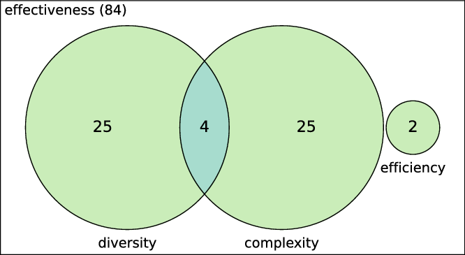
Figure 7. Distribution of objectives across EAs using multiple objectives. Effectiveness (predictive performance) is optimized in all 84 studies. From these, 56 work optimize another objective, be it diversity, complexity, or efficiency. Only four studies (Dos Santos et al. Reference Dos Santos, Sabourin and Maupin2008b; Cordón & Trawiński, Reference Cordón and Trawiński2013; Trawiński et al. Reference Trawiński, Cordón, Quirin and Sánchez2013; Ojha et al. Reference Ojha, Abraham and Snášel2017) optimize three objectives (effectiveness, diversity, and complexity), and no study optimizes all four at the same time.
In this work we follow the taxonomy of multi-objective optimization approaches proposed in Freitas (Reference Freitas2004), where approaches are categorized into three types: (i) weighted fitness functions, where each objective is assigned a user-defined (typically, very ad hoc) weight indicating that objective’s importance; (ii) the lexicographic approach, where the user only ranks the objectives in terms of their priorities (no ad hoc numerical weights), and then the EA selects individuals for reproduction by trying to optimize the objectives in their decreasing order of priority; and (iii) the Pareto dominance approach, where the EA evolves a set of non-dominated solutions in the Pareto sense—that is, a solution is non-dominated if it is not worse than any other according to each objective and it is better than others according to at least one objective.
In the surveyed papers, the least popular approach was the lexicographic one (Lima & Ludermir, Reference Lima and Ludermir2015), followed by weighted fitness functions (Park & Cho, Reference Park and Cho2003b; Coelho et al., Reference Coelho, Lima and Von Zuben2003; Kim & Cho, Reference Kim and Cho2005, Reference Kim and Cho2008a, 2015; Parhizkar & Abadi, Reference Parhizkar and Abadi2015a, 2015b; Hernández et al., Reference Hernández, Hernández, Cardoso and Jiménez2015; Winkler et al., Reference Winkler, Schaller, Dorfer, Affenzeller, Petz and Karpowicz2015; Zhang et al., Reference Zhang, Mistry, Neoh and Lim2016a; Liew et al., Reference Liew, Loo and Obo2017; Batista et al., Reference Batista, Rodrigues and Varejão2017), then the single-objective approach (see the single-objective entry in Table 7) and finally the Pareto dominance approach as the most popular one (all the papers that were not cited in this paragraph and are within the multi-objective entry in Table 7).
Table 7. Studies categorized by number and type of objectives employed

8. Types of evolutionary algorithms
A variety of EAs have been employed in ensemble learning. While some of these EAs are less frequent in literature (e.g., Flower Pollination Algorithm Zhang et al., Reference Zhang, Qu, Zhang, Mao, Ma and Fan2017a, Levy-Flight Firefly Algorithm Zhang et al., Reference Zhang, Mistry, Neoh and Lim2016a), others are more common. Among them, Genetic Algorithms (GAs) is the most popular, followed by Genetic Programming, and Differential Evolution.
Within GAs, apart from its vanilla version, Non-dominated Sorting Genetic Algorithm II (NSGA-II) is the most popular implementation. This choice seems due to NSGA-II’s ability to deal with multiple objectives, suiting well the multi-objective nature of ensemble learning. Table 8 shows the distribution of the surveyed studies according to the type of EA used.
Table 8. Studies organized by the type of EA employed, and the ensemble learning stage optimized

9. Types of base learners
In the surveyed studies, the most commonly used type of base learner is ANNs, used in 75 studies; followed by tree-based algorithms (e.g., decision trees, arithmetic trees), used in 48 studies; and SVMs, used in 46 studies. The number of studies using each type of base learner algorithm is shown in Table 9.
Table 9. Studies organized according to the base learners they employ. We only show in this table base learners that are present in at least 5 papers. For the complete list of base learners, please refer to our website at https://henryzord.github.io/eael

Some ensemble techniques are more appropriate for some type(s) of selected base learner(s). SVMs, for instance, are stable classifiers, making the techniques of selecting either instances or attributes for each base learner inefficient as a diversity inductor (Batista et al., Reference Batista, Rodrigues and Varejão2017).
The majority of the studies use homogeneous ensembles, as opposed to heterogeneous ones (113 vs. 47). Four work use both types of ensembles, which brings the count to 117 and 51, respectively. Figure 8 shows the base learners that were used in at least 5 studies, as well as the study’s ensemble type: either homogeneous, or heterogeneous.
Homogeneous ensembles are composed by the same base learner paradigm. However, this is not to say that all base learners are exactly the same. When using neural networks, those models can have distinct activation functions or topologies. According to Rahman and Verma (Reference Rahman and Verma2013c), there are five strategies for inducing diverse models in homogeneous ensembles: (i) post-model optimization (see Section 4.3); (ii) manipulation of the error function; (iii) distinct attribute subsets across base learners (see Section 4.2); (iv) manipulation of output targets, in which some instances in the training set have their class labels switched, for inducing diversity; and (v) distinct instance subsets across base learners (see Section 4.1). Strategies (ii) and (iv) are not covered in this survey, though, due to the lack of relevant papers.
Heterogeneous ensembles comprise base learners from distinct paradigms. As such, there is no pressure for inducing diversity in the ensemble, since learners from distinct paradigms tend to make diverse predictions. In our survey, among the studies using diversity measures, 19 have a homogeneous set of base learners, while 9 use a heterogeneous set. These numbers include a single paper that proposes both homogeneous and heterogeneous ensembles. The larger number of papers with homogeneous sets is probably because it is simpler to work with homogeneous ensembles than with heterogeneous ones. While Figure 8 depicts an overview of the number of studies per type of base learners, Table 10 identifies which studies are using which types of base learners, and also their configuration (homogeneous or heterogeneous). Note that a few studies (4) use both types of ensemble.

Figure 8. Types of base learners used in surveyed work, as well as their distribution.
Table 10. Studies organized according to the base learners’ homogeneity/heterogeneity

10. Algorithm complexity by stages of ensemble learning
As it is expected with a survey that broadly reviews the literature, it is difficult to derive a single algorithm complexity for Ensemble Learning with Evolutionary Algorithms, or even multiple accurate estimations. For this reason, in this section we will discuss what aspects have the most impact on algorithm complexity, as well as deriving a general complexity for relevant ensemble stages (i.e., generation and selection).
The most time-consuming step in an evolutionary algorithm is evaluating candidate solutions. How candidate solutions are built differs among EAs, but it is safe to assume that these solutions are, in the context of ensemble learning, already-built, ready-to-deploy ensembles. Consider for example a ‘generic’ evolutionary algorithm for the generation stage. Let us assume that this EA does not have a pool of base classifiers—that is, for each candidate solution, it builds base classifiers that will only be used by that solution. If this EA runs for G generations and has a population of S individuals, then the time complexity of this algorithm is
 $O(G \times ( B S \Psi \Omega) )$
, where B is the number of base classifiers in each ensemble (individual),
$O(G \times ( B S \Psi \Omega) )$
, where B is the number of base classifiers in each ensemble (individual),
 $\Psi$
is the complexity of the most time-consuming base classifier employed in the ensemble (in case it is heterogeneous), or the complexity of the only base classifier used (in case the ensemble is homogeneous), and
$\Psi$
is the complexity of the most time-consuming base classifier employed in the ensemble (in case it is heterogeneous), or the complexity of the only base classifier used (in case the ensemble is homogeneous), and
 $\Omega$
is the complexity of aggregating predictions among base classifiers.
$\Omega$
is the complexity of aggregating predictions among base classifiers.
 $\Omega$
can be as fast as O(B), when using majority voting, to an arbitrarily complex algorithm, such as employing Genetic Algorithms to evolve Expression Trees (presented in Section 6.2.1). When more than one aggregation policy is available, the reader should assume the worst case scenario—that is, that all solutions will take as much time to train as it takes to use the most time-consuming base classifiers, coupled with the most time-consuming aggregation policy.
$\Omega$
can be as fast as O(B), when using majority voting, to an arbitrarily complex algorithm, such as employing Genetic Algorithms to evolve Expression Trees (presented in Section 6.2.1). When more than one aggregation policy is available, the reader should assume the worst case scenario—that is, that all solutions will take as much time to train as it takes to use the most time-consuming base classifiers, coupled with the most time-consuming aggregation policy.
Note that having a pre-built pool of classifiers to choose from reduces the time complexity. In the case of a ‘generic’ EA for the selection stage, when the EA performs static selection, the time complexity is
 $O((P \times \Psi) + G \times (S \Omega))$
, where P is the pool size, and
$O((P \times \Psi) + G \times (S \Omega))$
, where P is the pool size, and
 $P \geq B$
(in this case, each individual will have a different B). Once base classifiers are built, their matrices of probabilities can be stored in memory and aggregated by any desired aggregation policy with
$P \geq B$
(in this case, each individual will have a different B). Once base classifiers are built, their matrices of probabilities can be stored in memory and aggregated by any desired aggregation policy with
 $\Omega$
complexity. Since static selection consists only in flipping bits in a binary vector, its complexity is negligible. On the other hand, the complexity of dynamic selection (presented in Section 5.2) lies on the complexity of training a selector to be later used during the prediction phase. In this case, the complexity of a generic EA performing dynamic selection is approximately
$\Omega$
complexity. Since static selection consists only in flipping bits in a binary vector, its complexity is negligible. On the other hand, the complexity of dynamic selection (presented in Section 5.2) lies on the complexity of training a selector to be later used during the prediction phase. In this case, the complexity of a generic EA performing dynamic selection is approximately
 $O((P \times \Psi) + G \times (S \Xi \Omega))$
, where
$O((P \times \Psi) + G \times (S \Xi \Omega))$
, where
 $\Xi$
is the complexity of learning that selector.
$\Xi$
is the complexity of learning that selector.
11. Conclusions and new research directions
Ensemble learning is an extensive research field due to the improvement it presents in comparison to single learners and the easiness to integrate within some challenging types of machine learning problems (e.g., data stream learning and datasets with imbalanced class distributions Krawczyk et al., Reference Krawczyk, Galar, Jeleń and Herrera2016; Folino et al., Reference Folino, Pisani and Sabatino2016; Mauša & Grbac, Reference Mauša and Grbac2017). For some problems, inducing a single, stronger-than-all base learner can be a difficult task (Almeida & Galvão, Reference Almeida and Galvão2016), while ensembles of models can perform better with regard to both effectiveness and efficiency (Breiman, Reference Breiman1996; Gu & Jin, Reference Gu and Jin2014; Oehmcke et al., Reference Oehmcke, Heinermann and Kramer2015; Parhizkar & Abadi, Reference Parhizkar and Abadi2015a; Krithikaa & Mallipeddi, Reference Krithikaa and Mallipeddi2016).
Ensemble learning can be further enhanced by using EAs in one or more of its learning stages: generation, selection, and integration. In this survey, we reviewed a large number of studies using many types of EAs for ensemble learning and proposed a taxonomy to classify such studies with regard to different aspects of ensemble learning. We also reviewed the debate on controversial topics, like the selection of ensemble members (rather than using all members) and the usefulness of optimizing a diversity measure for the members of the ensemble.
In order to facilitate the review of specific studies discussed in our survey, we make available the metadata used to compile our figures and tables. By using such metadata, one can see at a glance all the main aspects of a given study (e.g., which base learners, objectives, learning stages, etc, a study is using). The repository is available at https://github.com/henryzord/eael. We also provide a master table, in the form of a website, listing all surveyed work, and their classification according to our taxonomy: https://henryzord.github.io/eael.
11.1 Summary of findings
First, we discuss the main findings of this survey regarding each stage of the ensemble learning process. The generation stage, that is where the ensemble members are generated, was found to be the most popular step to employ EAs, having more studies dedicated to it than the selection and integration stages combined. Wrapper methods were found to be much more common than filter ones for the instance selection and attribute selection approaches. This seems natural, considering that, unlike filters, wrappers select attributes or instances customized for the supervised learning algorithm to be used later (to induce a model), which tends to improve predictive performance. However, wrappers are normally much slower than filters. Hence, in applications with large datasets or where efficiency is a critical factor, the filter approach deserves more attention. In addition, in the model tuning approach for generation, post-model optimization (used to improve an existing model) was found to be more popular than pre-model optimization (used before learning the model).
The next stage, selection—where ensemble members are selected to be used in the testing phase—is an optional stage, which is missing in many ensemble learning systems. In this stage, static selection, where the regions of competence of ensemble members are identified at training time, was found to be much more popular than dynamic selection, where those regions are identified at testing (prediction) time. This seems partly due to the greater simplicity and computational efficiency of the former, since dynamic selection in general requires a more time-consuming process of identifying regions of competence of ensemble members for each testing instance.
In the integration stage, where the predictions of the base learners are integrated into a final prediction for each instance, by far the most popular approach among the surveyed studies was the use of a first degree polynomial—a simple linear approach. Among the nonlinear integration techniques, the most common was the use of expression trees, using a genetic programming algorithm. It seems that more research is needed on nonlinear techniques for integration, in order to determine whether or not their higher computational complexity could be justified by a significant increase in predictive performance.
Regarding the number of objectives in the fitness function, multi-objective EAs were found to be much more common than single-objective ones. This seems natural, given the multi-objective nature of the ensemble learning problem. In terms of specific types of objectives, effectiveness (predictive performance) is used by all surveyed EAs, since it is essential. Diversity and complexity share a second place, despite diversity being a controversial objective, as discussed earlier. Finally, efficiency, the capacity to generate ensembles that are computationally fast, is optimized in only two studies. Efficiency is important in huge datasets (since the training process must eventually finish, and a compromise between time spent in training stage and effectiveness must be made), and in data stream scenarios, where data is treated not as a fixed batch of instances, but instead as a continuous flow. Efficiency and effectiveness are competing objectives, since efficiency prioritizes models that are faster to train (and thus more likely to be simpler, less accurate models). However, if efficiency is a priority, one could use techniques such as parallelization of one of evolutionary algorithms’ steps (Hauschild & Pelikan, Reference Hauschild and Pelikan2011) to alleviate this competition.
Regarding the main types of EAs used in the surveyed studies, the most popular one was by far Genetic Algorithms (often NSGA-II, a multi-objective GA), followed by Genetic Programming and Differential Evolution.
Regarding the main type of base learner, the most popular one was ANNs, followed by decision trees and SVMs. The popularity of ANNs as base learners seems partly due to a long history of interaction in the EA and ANN research areas and partly due to the nature of ANNs, whose performance can often be improved when using ensembles. However, learning ensembles of ANNs or SVMs tends to be very computationally expensive. This problem is mitigated when learning an ensemble of decision trees (much faster base learners).
11.2 New research directions
One direction for future research is the automated selection of the best combination of ensemble algorithms and their hyper-parameter settings for a given input dataset. This is a complex optimization problem because, as discussed earlier, there are many types of ensembles (e.g., bagging, boosting, stacking, etc), and for each type of ensemble, many types of base (classification or regression) algorithms can be chosen. In addition, both the ensemble type and its base algorithm type(s) typically have many hyper-parameters, whose settings also have a large influence on the ensemble’s predictive performance. All these choices of algorithms and hyper-parameter settings interact in a complex manner, and ideally all these choices should be made in a synergistic way, optimizing all these choices as a whole for the specific dataset provided as input by the user. Emerging research has addressed this complex optimization problem by doing a search in the space of different types of learning algorithms and their hyper-parameter settings, in order to automatically select the best combination of algorithm and hyper-parameter settings for an input dataset (Wistuba et al., Reference Wistuba, Schilling and Schmidt-Thieme2017; Kordík et al., Reference Kordík, Černý and Frýda2018). To the best of our knowledge, although there are several EA-based systems that address this problem by considering a search space with many types of supervised learning algorithms (e.g., Olson et al., Reference Olson, Bartley, Urbanowicz and Moore2016; de Sá et al., Reference de Sá, Pinto, Oliveira and Pappa2017), there are only two studies using an EA to address this problem by considering a search space focused on ensembles (Kordík et al., Reference Kordík, Černý and Frýda2018; Xavier-Júnior et al., Reference Xavier-Júnior, Freitas, Feitosa-Neto and Ludermir2018). This seems an area with good potential for research growth.
Also, it is yet to be seen a framework that provides a synergistic integration of two or more ensemble learning stages (generation, selection, and integration). Even when a study addresses two or more stages, this is not done synergistically; base learners are first generated and later selected, or first selected and later integrated. We are not aware of any EA addressing all three stages.
Finally, ensemble learning with EAs would benefit from a unified, generic-purpose software tool, similarly to what WEKA (Witten et al., Reference Witten, Frank, Hall and Pal2016) and scikit-learn (Pedregosa et al., Reference Pedregosa, Varoquaux, Gramfort, Michel, Thirion, Grisel, Blondel, Prettenhofer, Weiss, Dubourg, Vanderplas, Passos, Cournapeau, Brucher, Perrot and Duchesnay2011) do for machine learning in general and Tensorflow (Abadi et al., Reference Abadi, Agarwal, Barham, Brevdo, Chen, Citro, Corrado, Davis, Dean, Devin, Ghemawat, Goodfellow, Harp, Irving, Isard, Jozefowicz, Jia, Kaiser, Kudlur, Levenberg, Mané, Schuster, Monga, Moore, Murray, Olah, Shlens, Steiner, Sutskever, Talwar, Tucker, Vanhoucke, Vasudevan, Viégas, Vinyals, Warden, Wattenberg, Wicke, Yu and Zheng2015) for deep learning. This would greatly facilitate the task of comparing different strategies, for example, distinct approaches for generating or selecting base learners while keeping the same fitness function. We believe the development of such a framework to be a major step forward to the evolutionary ensemble learning community.
11.3 Further readings
While this work is, up to our knowledge, the first to present a broad review of evolutionary algorithms for ensemble learning, the following literature can give a better understanding on topics related to ensemble learning, not necessarily involving evolutionary algorithms.
A closely related work to ours is the one of Yao and Islam (Reference Yao and Islam2008), which present a review of evolutionary algorithms for ensemble learning, although focusing only in work that uses ANNs as base classifiers.
For a general comprehension on ensemble learning, not necessarily involving evolutionary algorithms, Sagi and Rokach (Reference Sagi and Rokach2018) presents recent, state-of-the-art methods for ensemble learning. This is an update of another review on ensemble learning of the same author, presented in the work of Rokach (Reference Rokach2010). While the former reviews generation and integration methods, as well as presenting the main challenges when building methods for ensemble learning, the later reviews integration and selection methods, and a discussion on ensemble diversity.
In the work of Oza and Tumer (Reference Oza and Tumer2008) the authors review ensemble methods for solving real-world problems, such as remote sensing, person recognition, and medicine applications. Athar et al. (Reference Athar, Butt, Anwar and Latif2017) review classifier ensembles for sentiment analysis. Data stream analysis with ensembles is reviewed both in the work of Gomes et al. (Reference Gomes, Barddal, Enembreck and Bifet2017) and Krawczyk et al. (Reference Krawczyk, Minku, Gama, Stefanowski and niak2017).
A broad review on classification ensembles and its applications is presented in Tabassum and Ahmed (Reference Tabassum and Ahmed2016), while a survey on regression ensembles is presented in Mendes-Moreira et al. (Reference Mendes-Moreira, Soares, Jorge and de Sousa2012).
Regarding the generation stage, Olvera-Lopez et al. (2010) presents a review on instance selection methods, which can be used in this stage of ensemble learning; while Debie et al. (Reference Debie, Shafi, Merrick and Lokan2016) review ensemble methods that focus on feature selection.
For the selection stage, Britto et al. (Reference Britto, Sabourin and Oliveira2014) presents a review on dynamic selection of classifiers, as well as a statistical comparison of results of the reviewed methods. An update of the reviewed methods, as well as the proposed taxonomy by the authors, is presented by Cruz et al. (Reference Cruz, Sabourin and Cavalcanti2018).
Acknowledgments
This study was financed in part by the Coordenação de Aperfeiçoamento de Pessoal de Nível Superior—Brasil (CAPES)—Finance Code 001. The authors would also like to acknowledge FAPERGS for partially funding this research.
Conflicts of interest
The authors declare none.


