


1. Introduction
The Kolmogorov theory of equilibrium cascade works best for statistically stationary and homogeneous turbulence where the power input balances the dissipation rate and predicts that the interscale transfer rate balances the turbulence dissipation rate in an inertial range of scales (Batchelor Reference Batchelor1953; Frisch Reference Frisch1995; Lesieur Reference Lesieur1997). In particular, this inertial range equilibrium cascade leads to the well-known turbulence dissipation scaling (Batchelor Reference Batchelor1953; Sreenivasan Reference Sreenivasan1984; Vassilicos Reference Vassilicos2015) first introduced by Taylor (Reference Taylor1935) without justification. In statistically homogeneous but non-stationary, in particular decaying, turbulence, the situation is different. Specifically, there is a non-equilibrium turbulence dissipation scaling initially during decay (Vassilicos Reference Vassilicos2015; Goto & Vassilicos Reference Goto and Vassilicos2016), followed at later times by the classical turbulence dissipation as a result of balanced non-equilibrium (Goto & Vassilicos Reference Goto and Vassilicos2016; Steiros Reference Steiros2022) rather than Kolmogorov equilibrium throughout an inertial range.
Lundgren (Reference Lundgren2002) applied a matched asymptotic expansion approach to freely decaying homogeneous isotropic turbulence far from initial conditions, which led to the conclusion that the interscale transfer rate has an extremum at a length scale  $r_{max}$ that is proportional to the Taylor length
  $\lambda$. Wind tunnel data of nominally freely decaying homogeneous isotropic turbulence (Obligado & Vassilicos Reference Obligado and Vassilicos2019) confirm
  $r_{max} \approx 1.5 \lambda$ and EDQNM simulations of such turbulence (Meldi & Vassilicos Reference Meldi and Vassilicos2021) confirm
  $r_{max} \approx 1.12 \lambda$ for
  $Re_{\lambda } = 10^{2}$ to
  $10^{6}$. Hence, Kolmogorov equilibrium in non-stationary, in fact freely decaying far from initial conditions, statistically homogeneous isotropic turbulence seems to be achieved asymptotically only around
  $\lambda$; and not in an inertial range given that
  $\lambda$ depends on viscosity and total turbulent kinetic energy, and that there is a systematic departure from equilibrium (most clearly demonstrated in Meldi & Vassilicos Reference Meldi and Vassilicos2021) when moving away from
  $\lambda$, both towards the integral scale and towards the Kolmogorov length
  $\eta$.
Diverting attention from homogeneous non-stationary turbulence to stationary non-homogeneous turbulence, we ask about the validity of Kolmogorov equilibrium in stationary non-homogeneous conditions and chose to focus in this paper on fully developed turbulent channel flow (FD TCF). This is a statistically stationary non-homogeneous turbulent flow where turbulence production approximately balances turbulence dissipation (similarly to statistically stationary homogeneous turbulence) in some very significant region of space, the intermediate layer where the log-law of the wall has been traditionally claimed. Is there an average equilibrium between interscale turbulence energy transfer rate and turbulence dissipation in the intermediate layer of FD TCF where turbulence production approximately balances turbulence dissipation? If so, in what range of length scales, inertial or not? What processes are involved in the scale-by-scale turbulence energy balance in that range, if there is one, and outside it? What is the role of inhomogeneity, in particular in terms of scale-by-scale turbulence production but also directly on interscale energy transfer? What type of flow motions underpin interscale turbulence energy transfers and scale-by-scale turbulence production (referred to as two-point turbulence production in the remainder of this paper)?
In the following section, we introduce the scale-by-scale turbulence energy balance in its most general form and the spherical average operation, which we use to simplify it for this study. Section 3 is a brief description of the FD TCF DNS data we use for our post-processing. In § 4, we simplify the spherically averaged scale-by-scale turbulence energy balance for the particular case of the intermediate layer of an FD TCF and in § 5, we examine the two-point turbulence production term which appears in this balance. Section 6 deals with second- and third-order structure functions and interscale turbulence energy transfer by adapting to FD TCF the matched asymptotic expansion approach of Lundgren (Reference Lundgren2002), and then we compare the results to the DNS data in § 7. Finally, § 8 introduces two decompositions of the interscale turbulence energy transfer rate and attempts to answer the questions of non-homogeneity's role and of what flow motions are responsible for which aspects of interscale turbulence energy transfer. In § 9, we summarise our conclusions.
2. Scale-by-scale turbulence energy balance
To analyse the turbulent energy cascade in turbulent channel flow, we use a Kármán–Howarth–Monin–Hill (KHMH) equation which is a scale-by-scale energy budget equation in its most general form without any assumptions about the flow (Hill Reference Hill2001, Reference Hill2002). The form of the KHMH equation that we use is an evolution equation for  $|\delta \boldsymbol {u}|^2$, where
  $\delta \boldsymbol {u} \equiv \boldsymbol {u}(\boldsymbol {x} + \boldsymbol {r}/2, t) - \boldsymbol {u}(\boldsymbol {x}-\boldsymbol {r}/2,t)$ is the difference between fluctuating velocities at two points
  $\boldsymbol {\xi }^{+} \equiv \boldsymbol {x} + \boldsymbol {r}/2$ and
  $\boldsymbol {\xi }^{-} \equiv \boldsymbol {x} - \boldsymbol {r}/2$ in the flow where the separation vector
  $\boldsymbol {r}=(r_1,r_2,r_3)$ gives some sense of scales. The centroid
  $\boldsymbol {x}=(x_{1}, x_{2}, x_{3})$ is mid-way between these two points.
A Reynolds decomposition  $\boldsymbol {U} + \boldsymbol {u}$ is used for the velocity field in this form of the KHMH equation where
  $\boldsymbol {U} = (U_1,U_2,U_3)$ is the mean flow. The KHMH equation follows directly from the incompressible Navier–Stokes equations and, with notation
  $U_{i}^{\pm } \equiv U_{i}(\boldsymbol {x} \pm \boldsymbol {r}/2)$,
  $u_{i}^{\pm } \equiv u_{i}(\boldsymbol {x} \pm \boldsymbol {r}/2)$ and
  $\delta p \equiv p(\boldsymbol {x} + \boldsymbol {r}/2, t) - p (\boldsymbol {x}-\boldsymbol {r}/2,t)$, where
  $p$ is the fluctuating pressure field (normalised by the constant density), reads as follows:

where the brackets  $\langle {\cdot } \rangle$ denote the averaging operation on which the Reynolds decomposition is based. The KHMH equation includes the following terms:
(i)
 $A_t = {\partial \langle |\delta \boldsymbol {u}|^2 \rangle }/{\partial t}$ is the time derivative term;
(ii)
$A = {(U_i^{+} + U_i^{-})}/{2})({\partial \langle |\delta \boldsymbol {u}|^2 \rangle }/{\partial x_i})$ is the mean advection term;(iii)
$\varPi = {\partial \langle \delta u_i |\delta \boldsymbol {u}|^2 \rangle }/{\partial r_i}$ is the nonlinear interscale transfer rate of $|\delta \boldsymbol {u}|^2$ by turbulent fluctuations in scale space and thus directly linked to the energy cascade;(iv)
$\varPi _U={\partial \delta U_i \langle |\delta \boldsymbol {u}|^2 \rangle }/{\partial r_i}$ is the linear interscale transfer rate of $|\delta \boldsymbol {u}|^2$ in scale space by mean velocity differences;(v)
$\mathcal {P}\,{=}\,{-}2\langle \delta u_i \delta u_j \rangle ({\partial \delta U_j}/{\partial r_i})\,{-}\,\langle (u_i^{+} \,{+}\, u_i^{-})\delta u_j \rangle ({\partial \delta U_j}/{\partial x_i})$ is the two-point production of $|\delta \boldsymbol {u}|^2$ by the mean shear;(vi)
$T_u={\partial \langle ({(u_i^{+} + u_i^{-})}/{2})|\delta \boldsymbol {u}|^2 \rangle }/{\partial x_i}$ is the turbulent transport of $|\delta \boldsymbol {u}|^2$ in physical space;(vii)
$T_p=2({\partial \langle \delta u_i \delta p \rangle }/{\partial x_i})$ is the pressure-velocity term;(viii)
$D_x=({\nu }/{2}) ({\partial ^2 \langle |\delta \boldsymbol {u}|^2 \rangle }/{\partial x_i^2})$ is the viscous diffusion in physical space;(ix)
$D_r=2 \nu ({\partial ^2 \langle |\delta \boldsymbol {u}|^2 \rangle }/{\partial r_i^2})$ is the viscous diffusion in scale space;(x)
$\varepsilon = 2\nu \langle ( \partial u^{-}_j/\partial \xi _i^{-} )^{2}\rangle + 2\nu \langle ( \partial u_j^{+}/\partial \xi _i^{+} )^{2}\rangle$ is the two-point averaged turbulence pseudo-dissipation rate which is very close to the actual turbulence dissipation rate (e.g. see Pope Reference Pope2000).


At this stage, we specialise this equation to FD TCF by choosing the averaging operation  $\langle {\cdot } \rangle$ to be over the streamwise and spanwise homogeneous directions, i.e. over coordinates
  $x\equiv x_{1}$ (streamwise) and
  $z\equiv x_{3}$ (spanwise), and over time. The wall-normal coordinate is
  $y\equiv x_{2}$. Note that
  $U_{2}=U_{3}=0$ and that this averaging operation implies
  $A_t =0=A$. In non-homogeneous and non-isotropic turbulent flows (such as FD TCF), energy transfers and exchanges, including the turbulence cascade, are anisotropic. This equation has been studied extensively in FD TCF by Marati, Casciola & Piva (Reference Marati, Casciola and Piva2004), Cimarelli & De Angelis (Reference Cimarelli and De Angelis2012), Cimarelli, De Angelis & Casciola (Reference Cimarelli, De Angelis and Casciola2013), Cimarelli et al. (Reference Cimarelli, De Angelis, Jimenez and Casciola2016) and Gatti et al. (Reference Gatti, Remigi, Chiarini, Cimarelli and Quadrio2019). In this paper, we concentrate our interest on the directionally averaged energy transfers by applying to each term of the KHMH equation an additional average over spheres in
  $\boldsymbol {r}$-space. We therefore work with
 \begin{equation} \varPi^{v} + \varPi_{U}^{v} = \mathcal{P}^{v} + T_{u}^{v} + T_{p}^{v} + D_{x}^{v} + D_{r}^{v} -\varepsilon^{v}, \end{equation}
where (following Zhou & Vassilicos (Reference Zhou and Vassilicos2020) and § 2 of Chen & Vassilicos (Reference Chen and Vassilicos2022)) every term is obtained from its analogue in (2.1) by the application of the normalised three-dimensional (3-D) integral  $({3}/{4{\rm \pi} r^{3}})\int _{S(r)} {\rm d}^{3} \boldsymbol {r}$,
  $S(r)$ being the sphere of radius
  $r$ in
  $\boldsymbol {r}$-space; for example,
  $\varPi ^{v} \equiv ({3}/{4{\rm \pi} r^{3}})\int _{S(r)} \varPi \,{\rm d}^{3} \boldsymbol {r}$,
  $\varPi _{U}^{v} \equiv ({3}/{4{\rm \pi} r^{3}})\int _{S(r)} \varPi _{U}\,{\rm d}^{3} \boldsymbol {r}$,
  $\mathcal {P}^{v} \equiv ({3}/{4{\rm \pi} r^{3}})\int _{S(r)} \mathcal {P}\,{\rm d}^{3} \boldsymbol {r}$, etc.
This approach averages over and therefore ignores length-scale anisotropies and replaces  $\boldsymbol {r}$ by its modulus
  $r=|\boldsymbol {r}|$ as a single measure of length-scale. However, the fundamental anisotropy responsible for correlations between streamwise and wall-normal directions remains in the turbulence production term. Every term in (2.2) is a function of only
  $y$ (spatial non-homogeneity variable) and
  $r$ (length-scale variable).
In § 3, we describe the data from direct numerical simulations (DNS) of FD TCF that we use in this paper. We describe these DNS data before starting our analysis of (2.2) to be able to test against these data certain aspects of our analysis as it proceeds.
3. DNS data
For our analysis, we use the DNS data of Lozano-Durán & Jiménez (Reference Lozano-Durán and Jiménez2014) for FD TCF at  $Re_\tau =932 \textrm { and } 2003$, (
 $Re_{\tau }\equiv u_{\tau } \delta /\nu$, where
  $\nu$ is the kinematic viscosity,
  $\delta$ is the channel half-width, and
  $u_{\tau }$ is the skin friction velocity obtained by averaging over time and over streamwise coordinate
  $x$ and spanwise coordinate
  $z$ at the channel's solid wall
  $y=0$). The domain size for both simulations is
  $L_x=2{\rm \pi} \delta$ in the streamwise and
  $L_z={\rm \pi} \delta$ in the spanwise directions. The Navier–Stokes equations have been solved by integrating the evolution equations in terms of the wall-normal vorticity and the Laplacian of the wall-normal velocity for an incompressible fluid. The Fourier spectral method was used for the spatial discretisation in the wall-parallel directions. For the discretisation in the wall-normal direction, Chebyshev polynomials were used in the
  $Re_\tau =932$ case, whereas a seven-point compact finite difference scheme was used in the
  $Re_\tau =2003$ case. Finally, a third-order semi-implicit Runge–Kutta method with
  $\textrm {CFL}=0.5$ was chosen for time advancement. A comparison of the two datasets can be found in Table 1 (the superscript
  $^+$ refers to non-dimensionalisation with wall units
  $\delta _{\nu }\equiv \nu /u_{\tau }$ for length and
  $\delta _{\nu }/u_{\tau }$ for time). We focus our DNS data analysis on the wall-normal locations that correspond to the region where the average production rate of turbulent kinetic energy roughly balances the average turbulence dissipation rate as identified by Apostolidis, Laval & Vassilicos (Reference Apostolidis, Laval and Vassilicos2022), i.e.
  $60\le y^{+}\le Re_{\tau }/2$.
Table 1. DNS databases.

4. Scale-by-scale turbulent energy balance in the one-point average equilibrium range of FD TCF
We now examine (2.2) in the region of FD TCF, where the average one-point turbulence production rate is in approximate equilibrium with the average turbulence dissipation rate at a given  $y$. This is a region of distances
  $y$ from the bottom wall (where
  $y=0$) such that
  $\delta _{\nu } \ll y \ll \delta$ (in the limit
  $Re_{\tau }=\delta /\delta _{\nu }\gg 1$) and where, classically, the mean flow velocity
  $\boldsymbol {U} = (U_1,0,0)$ is expected to be logarithmic (e.g. see Pope Reference Pope2000). Whilst previous works have suggested some not insignificant deviations from a log dependence on
  $y$ of
  $U_1$ (e.g. see Vassilicos et al. Reference Vassilicos, Laval, Foucaut and Stanislas2015), in this work, we assume that the log law accounts for most of
  $U_1$, which implies that
  $\varPi _U = ({\partial }/{\partial r_{1}}) (\delta U_{1} \langle |\delta \boldsymbol {u}|^2 \rangle )$ is close to
  $0$ in the region
  $\delta _{\nu } \ll y \ll \delta$ if
  $r_{2}\ll 2y$ because
  $\delta U_{1} = ({u_{\tau }}/{\kappa }) \ln {(1+r_{2}/y)}/{(1-r_{2}/y)} \approx 0$ (
 $\kappa$ is the von Kármán dimensionless coefficient and note that wall blocking implies that
  $r_2$ is necessarily smaller or equal to
  $2y$). The DNS data confirm the prediction that
  $\varPi ^{v}_U$ is close to zero, see figure 1(c,d). We also make the assumption that turbulence is well mixed in this region and therefore assume that the physical-space divergence term
  $T_{u}^{v} + T_{p}^{v}$ is negligible. Whilst the DNS data support this assumption, see figure 1(a,b), it must be stressed that pressure plays an important redistributive role and that spatial energy transfer is not fully absent in the intermediate layer (e.g. Lozano-Durán & Jiménez Reference Lozano-Durán and Jiménez2014; Cimarelli et al. Reference Cimarelli, De Angelis, Jimenez and Casciola2016; Lee & Moser Reference Lee and Moser2019). The numerical details behind our calculations of normalised 3-D integrals
  $({3}/{4{\rm \pi} r^{3}})\int _{S(r)} {\rm d}^{3} \boldsymbol {r}$, and in particular of terms such as
  $T_{u}^{v} = ({3}/{4{\rm \pi} r^{3}})\int _{S(r)} T_{u}\,{\rm d}^{3} \boldsymbol {r}$ and
  $T_{p}^{v}=({3}/{4{\rm \pi} r^{3}})\int _{S(r)} T_{p} \,{\rm d}^{3} \boldsymbol {r}$, are given in the Appendix.

Figure 1. (a) Turbulent transport  $T_u$ plus pressure-velocity term
  $T_p$, integrated over the volume of sphere with radius
  $r$, normalised by the volume integral of the two point dissipation rate
  $\varepsilon$ as a function of
  $r/\lambda$ for
  $Re_\tau =932$, (b)
  $T_u^{v}/\varepsilon ^{v}$ for
  $Re_\tau =2003$ (
 $T_p$ is unavailable from the recorded DNS data at
  $Re_{\tau }=2003$), (c) volume integral of linear interscale transfer term divided with
  $\varepsilon ^{v}$
  $\varPi _U^{v}/\varepsilon ^{v}$ for
  $Re_\tau =932$ and (d) for
  $Re_\tau =2003$. Wall-normal distance is increased from light to dark colours (
 $y^{+}=59$ to
  $377$ for
  $Re_{\tau }=932$,
  $y^{+}=82$ to
  $665$ for
  $Re_{\tau }=2003$). The normalisation by the Taylor length
  $\lambda$ (defined in § 6.3) is arbitrary in these plots.
We therefore neglect both  $\varPi _U^v$ and
  $T_{u}^{v} + T_{p}^{v}$ from (2.2) and are left with
 \begin{equation} \varPi^{v} \approx \mathcal{P}^{v} + D_{x}^{v} + D_{r}^{v} -\varepsilon^{v} \end{equation}
for  $r_{2}\ll 2y$ in the intermediate layer
  $\delta _{\nu } \ll y \ll \delta$.
By application of the Gauss divergence theorem, the interscale transfer rate takes the form
 \begin{equation} \varPi^{v}= \frac{3}{4 {\rm \pi}} \int \left\langle \frac{\delta \boldsymbol{u}\boldsymbol{\cdot} \hat{\boldsymbol{r}}}{r}\vert \delta \boldsymbol{u}\vert^2\right\rangle \,{\rm d}\varOmega_{r}\equiv \frac{S_{3}(r,y)}{r}, \end{equation}
where  $\varOmega _r$ is the solid angle in
  $\boldsymbol {r}$ space and
  $\hat {\boldsymbol {r}}\equiv \boldsymbol {r}/|\boldsymbol {r}|$. By distinguishing between radial and solid angle integrations in
  $\boldsymbol {r}$-space, the viscous diffusion terms become
 \begin{equation} D_{x}^{v} + D_{r}^{v} = \frac{3\nu}{8{\rm \pi} r^{3}}\int_{0}^{r} \rho^{2} \frac{{\rm d}^{2}S_{2}}{{{\rm d}y}^{2}} (\rho, y) \,{\rm d}\rho+ \frac{3\nu}{{\rm \pi} r}\frac{{\rm d} S_{2}}{{\rm d} r}(r,y),\end{equation}
where
 \begin{equation} S_{2}(r,y) \equiv \int \langle \vert \delta \boldsymbol{u}\vert^{2}\rangle \,{\rm d}\varOmega_{r}. \end{equation}
In FD TCF, the production term  $\mathcal {P}^{v}$ is obtained by applying the integral operation
  $({3}/{4{\rm \pi} r^{3}})\int _{S(r)} {\rm d}^{3} \boldsymbol {r}$ on
  $-2 \langle \delta u_{2} \delta u_{1}\rangle ({\partial \delta U_{1}}/{\partial r_{2}}) - \langle (u_{2}^{+}+u_{1}^{-})\delta u_{1}\rangle ({\partial \delta U_{1}}/{\partial y})$. Targeting again the intermediate region
  $\delta _{\nu }\ll y \ll \delta$, where the log law
  ${{\rm d} U_{1}}/{{\rm d}y} \approx {u_{\tau }}/{\kappa y}$ might be considered to be a good approximation in the limit
  $\delta /\delta _{\nu }\gg 1$ (
 $\kappa$ is the von Kármán dimensionless coefficient), the two-point production term becomes
 \begin{equation} \mathcal{P}^{v}\approx{-}\frac{u_{\tau}^{3}}{\kappa y} \frac{3}{4{\rm \pi} r^{3}}\int_{0}^{r} \rho^{2} \left[\frac{S_{12}(\rho,y)}{u_{\tau}^{2}} - \frac{S_{1 \times 2}(\rho,y)}{u_{\tau}^{2}}\right]{\rm d}\rho \end{equation}
in this intermediate region, where
 \begin{equation} S_{12}(r,y)\equiv 2 \int \langle \delta u_{2} \delta u_{1}\rangle \left[1-\left(\frac{r_{2}}{2y}\right)^{2}\right]^{{-}1} {\rm d}\varOmega_{r} \end{equation}
and
 \begin{equation} S_{1 \times 2}(r,y)\equiv \int \langle(u_{2}^{+}+u_{2}^{-}) \delta u_{1}\rangle (r_{2}/y) \left[1-\left(\frac{r_{2}}{2y}\right)^{2}\right]^{{-}1}{\rm d}\varOmega_{r}. \end{equation}
 We expect  $S_{1 \times 2}(r,y)$ to be much smaller in magnitude than
  $S_{12}(r,y)$, in fact even close to vanishing, because of the expected decorrelation between wall-normal velocity fluctuations effectively larger than
  $r$ (i.e.
  $u_{2}^{+}+u_{2}^{-}$) and streamwise velocity fluctuations effectively smaller than
  $r$ (i.e.
  $\delta u_{1}$). This is confirmed by the DNS data in figure 2, which also show that
  $S_{12}(r,y)$ is negative for all
  $r\le 2y$ irrespective of
  $y$ (because of wall blocking,
  $r$ cannot be larger than
  $2y$, and because of the integrand's singularity in the definitions of
  $S_{1 \times 2}(r,y)$ and
  $S_{12}(r,y)$, we plot them for
  $r\le 2y-8\delta _{\nu }$ throughout the paper). In the intermediate region, where the log law of the wall might be expected to hold, we therefore have a positive two-point production term given, to good approximation, by
 \begin{equation} \mathcal{P}^{v}\approx{-}\frac{u_{\tau}^{3}}{\kappa y} \frac{3}{4{\rm \pi} r^{3}}\int_{0}^{r} \rho^{2} \frac{S_{12}(\rho,y)}{u_{\tau}^{2}}{\rm d}\rho. \end{equation}
Figure 2. Ratios of  $S_{1\times 2}$ in orange colours and
  $S_{2}$ in marine colours over
  $S_{12}$ for different normalised scales
  $r/y$. Wall-normal distance is increased from light to dark colours as in figure 1. (a)
  $Re_\tau =932$, (b)
  $Re_\tau =2003$.
Bringing together (4.2), (4.3) and (4.8) into (4.1), we obtain the following two-point energy balance valid for  $r_{2}\ll 2y$ and
  $\delta /\delta _{\nu }\gg 1$ in the intermediate region
  $\delta _{\nu }\ll y\ll \delta$ of FD TCF:
 \begin{align} & \frac{S_{3}(r,y)}{r} - \frac{3\nu}{8{\rm \pi} r^{3}}\int_{0}^{r} \rho^{2} \frac{{\rm d}^{2}S_{2}}{{{\rm d}y}^{2}} (\rho, y) \,{\rm d}\rho + \frac{3\nu}{{\rm \pi} r} \frac{{\rm d} S_{2}}{{\rm d} r}(r,y) \nonumber\\ &\quad \approx{-}\varepsilon^{v} -\frac{u_{\tau}^{3}}{\kappa y} \frac{3}{4{\rm \pi} r^{3}}\int_{0}^{r} \rho^{2}S_{12}(\rho,y)\,{\rm d}\rho. \end{align}
In this equation, the first term on the left-hand side is the interscale transfer rate, the second and third terms on the left-hand side are the viscous diffusion terms, and the second term on the right-hand side is the two-point turbulence production rate. Before making use of this equation in § 6, we look closer into the positive sign of the two-point turbulence production.
5. Two-point turbulence production
Here,  $\mathcal {P}^{v}$ represents the rate with which turbulent kinetic energy is gained or lost by scales smaller than
  $r$ if
  $\mathcal {P}^{v}$ is respectively positive or negative. Of course, we may expect energy to be gained in some
  $\boldsymbol {r}$ directions and lost in some other
  $\boldsymbol {r}$ directions:
  $\mathcal {P}^{v}$ represents the rate with which the aggregate energy averaged over all directions is gained or lost at scales smaller than
  $r$ by the linear effects of mean flow gradients on the turbulence. This is not a nonlinear interscale mechanism relating to a turbulence cascade which is, in fact, represented by
  $\varPi ^{v}$.
Turbulence production results from the interplay of non-isotropy in the form of non-zero Reynolds shear stresses with the mean flow gradient. In FD TCF, the one-point Reynolds shear stress is  $\langle u_{1} u_{2}\rangle$ and it interacts with the mean flow gradient
  ${{\rm d} U_{1}}/{{\rm d} x_{2}}={{\rm d} U_{1}}/{{\rm d}y}$ to give the one-point turbulence production rate
  $-\langle u_{1} u_{2}\rangle ({{\rm d} U_{1}}/{{\rm d}y}$) which is positive (i.e. creation of turbulent kinetic energy) because
  $\langle u_{1} u_{2}\rangle$ is negative. The negative sign of
  $\langle u_{1} u_{2}\rangle$ results from the predominance of turbulent transport towards the wall of forward streamwise fluctuating velocities and of turbulent transport away from the wall of backward streamwise fluctuating velocities. These turbulent momentum fluxes are partly caused by sweeps in the case of transport towards the wall and ejections in the case of transport away from the wall (Kline & Robinson Reference Kline and Robinson1990; Wallace Reference Wallace2016) and lead to the well-known increase by turbulence of wall shear stress and skin friction drag.
The two-point Reynolds shear stress  $\langle \delta u_{1}\delta u_{2}\rangle$ results from anisotropies at scales comparable to
  $r$ and smaller, and relates to the one-point shear stress by
 \begin{equation} \langle \delta u_{1}\delta u_{2}\rangle = (\langle u_{1}^{+}u_{2}^{+}\rangle - \langle u_{1}^{+}u_{2}^{-}\rangle) +(\langle u_{1}^{-}u_{2}^{-}\rangle - \langle u_{1}^{-}u_{2}^{+}\rangle).\end{equation}
One can expect the two-point Reynolds shear stress to have the same sign as the one-point shear stresses at  $\boldsymbol {\xi }^{+}$ and
  $\boldsymbol {\xi }^{-}$ (which are known to be negative in FD TCF) if the magnitudes of the two-point correlations
  $\langle u_{1}^{+}u_{2}^{-}\rangle$ and
  $\langle u_{1}^{-}u_{2}^{+}\rangle$ are decreasing functions of distance between
  $\boldsymbol {\xi }^{+}$ and
  $\boldsymbol {\xi }^{-}$. The two-point Reynolds shear stress appears in the two-point turbulence production rate via
  $S_{12}$ (see (4.8) and the definition in (4.6) of
  $S_{12}$) and we therefore define, for initial simplicity of interpretation, a two-point Reynolds shear stress integrated over the solid angle in
  $\boldsymbol {r}$-space as follows:
  $\tilde {S}_{12}(r,y)\equiv \int \langle \delta u_{2} \delta u_{1}\rangle \,{\rm d}\varOmega _{r}$. Defining additionally
  $\int \langle u_{2}^{+} u_{1}^{+}\rangle \,{\rm d}\varOmega _{r}= \int \langle u_{2}^{-} u_{1}^{-}\rangle \,{\rm d}\varOmega _{r}\equiv \tilde {R}_{12}(y,r)$ and
  $\int \langle u_{2}^{+} u_{1}^{-}\rangle \,{\rm d}\varOmega _{r}= \int \langle u_{2}^{-} u_{1}^{+}\rangle \,{\rm d}\varOmega _{r} \equiv \tilde {C}_{12}(r,y)$, (5.1) leads to
 \begin{equation} \tilde{S}_{12}(r,y) = 2\tilde{R}_{12}(y,r) -2\tilde{C}_{12}(r,y)\end{equation}
in terms of solid angle-integrated one-point Reynolds shear stress  $\tilde {R}_{12}(y,r)$ and solid angle-integrated two-point correlation
  $\tilde {C}_{12}(r,y)$. In figure 3(a,b), we use the DNS data to plot
  $\tilde {C}_{12}(r,y)/\vert \tilde {R}_{12}(y)\vert$ vs
  $r$ (black lines) for the two Reynolds numbers available and for different values of wall distance
  $y$. In all cases,
  $\tilde {C}_{12}(r,y)/\vert \tilde {R}_{12}(y,r)\vert$ is a monotonically increasing function of
  $r$, from
  $\tilde {C}_{12}(r,y)/\vert \tilde {R}_{12}(y,r)\vert = -1$ at
  $r=0$ towards
  $0$ with increasing
  $r$. It follows from (5.2) that the solid angle-integrated two-point Reynolds stress inherits the negative sign of the solid angle-integrated one-point Reynolds shear stress but with reduced magnitude because of the negative two-point correlation
  $\tilde {C}_{12}(r,y)$, which is smaller in magnitude than
  $\tilde {R}_{12}(y,r)$ for all
  $y$ and all
  $r\not = 0$.

Figure 3. (a,b)  $\tilde {C}_{12}/\vert \tilde {R}_{12}\vert$ integrated over the whole sphere in black lines, conditionally integrated over anti-aligned pairs in blue lines and conditionally integrated over aligned pairs in red lines: (a)
  $Re_\tau =932$; (b)
  $Re_\tau =2003$. (c,d) Similarly for
  ${C}_{12}/\vert {R}_{12}\vert$. Wall-normal distance is increased from light to dark colours as in figure 1.
Inheriting the sign of the one-point Reynolds shear stress means that for the two-point Reynolds shear stress, sweeps and ejections are contributing to its negative sign. However, the two-point correlation  $\tilde {C}_{12}(r,y)$ reduces the proportion of this contribution. Assuming that fluctuating velocities may be approximately aligned within sweep and ejection events, particularly for the smaller values of
  $r$, we now use the DNS data to calculate correlations between
  $u_{2}$ and
  $u_{1}$ at two different points
  $\boldsymbol {\xi }^{+}$ and
  $\boldsymbol {\xi }^{-}$ conditionally on
  $\boldsymbol {u}^+ \boldsymbol {\cdot } \boldsymbol {u}^{-}>0$ for aligned pairs of fluctuating velocities and conditionally on
  $\boldsymbol {u}^+ \boldsymbol {\cdot } \boldsymbol {u}^{-}<0$ for anti-aligned pairs. We compute the resulting solid angle-integrated conditional correlations which we plot in figure 3(a,b) normalised by
  $\vert \tilde {R}_{12}(y,r)\vert$, and identify them by
  $(\rightrightarrows )$ for the aligned and
  $(\rightleftarrows )$ for the anti-aligned condition. For both Reynolds numbers and for all wall distances tested, the conditional correlations are increasing functions of
  $r$, but positive when the condition is anti-alignment and negative when the condition is alignment. Anti-alignment, which is not so expected within sweeps and ejections (but may be linked to sweep-ejection pairs), increases the magnitude of the negative value of
  $\tilde {S}_{12}(r,y)$, particularly at the larger separations
  $r$, whereas alignment, presumably more present within sweeps and ejections, actually contributes to reduce the magnitude of the negative value of
  $\tilde {S}_{12}(r,y)$. As a result, the part of
  $-\tilde {S}_{12}(r,y)$ that is conditional on aligned fluctuating velocities is smaller than the part of
  $-\tilde {S}_{12}(r,y)$ that is conditional on anti-aligned fluctuating velocities, particularly at values of
  $r$ larger than the Taylor length-scale (see figure 4). The actual role of the Taylor length appears in § 6.

Figure 4. (a,b)  $\tilde {S}_{12}$ integrated over the whole sphere in black lines, conditionally integrated over anti-aligned pairs in blue lines and conditionally integrated over aligned pairs in red lines: (a)
  $Re_\tau =932$; (b)
  $Re_\tau =2003$. (c,d) Similarly for
  ${S}_{12}$. Wall-normal distance is increased from light to dark colours as in figure 1. The Taylor length
  $\lambda$ is defined in § 6.3.
The two-point Reynolds shear stress determines two-point turbulence production via  $S_{12}(r,y)$ in the intermediate
  $y$-region (see (4.8)). Our results on
  $\tilde {S}_{12}(r,y)$,
  $\tilde {R}_{12}(y,r)$ and
  $\tilde {C}_{12}(r,y)$ and their signs carry over qualitatively to
  $S_{12}(r,y)$,
  $R_{12} \equiv 2 \int \langle u_{2}^{+} u_{1}^{+} \rangle [1-({r_{2}}/{2y})^{2}]^{-1}\,{\rm d}\varOmega _{r}$ and
  $C_{12}(r,y) \equiv 2 \int \langle u_{2}^{+} u_{1}^{-} \rangle [1-({r_{2}}/{2y})^{2}]^{-1}\,{\rm d}\varOmega _{r}$ (with differences only at values of
  $r$ close to
  $2y$ because of the factor
  $[1-({r_{2}}/{2y})^{2}]^{-1}$ in the integrands which tends to infinity for
  $r_{2} \to 2y$, see figures 3(c,d) and 4(c,d) and compare them respectively with figures 3(a,b) and 4(a,b)). The two-point turbulence production is therefore positive for all
  $r\le 2y$ and all
  $y$ in the intermediate range mainly because one-point turbulence production is positive even though two-point correlations conditioned on aligned fluctuating velocities act to reduce this positivity. Two-point correlations conditioned on anti-aligned fluctuating velocities enhance the positive two-point turbulence production particularly at the larger separations
  $r$.
$r$.
6. Interscale transfer rate
Having analysed the production term in the scale-by-scale turbulence energy balance (4.1), we now turn our attention to the interscale transfer rate (4.2) and the viscous diffusion terms (4.3). We adapt to the scale-by-scale turbulence energy balance (4.9) (which we derived from (4.1)) the matched asymptotic expansion approach that Lundgren (Reference Lundgren2002) used to study freely decaying homogeneous isotropic turbulence, a very different flow from FD TCF.
The starting point is the hypothesis that  $S_2$,
  $S_3$ and
  $S_{12}$ have similarity forms, namely,
 $$\begin{gather} S_{2} (r,y) = v^{2}(y) s_{2}(r/l(y),y), \end{gather}$$
 $$\begin{gather}S_{3} (r,y) = v^{3}(y) s_{3}(r/l(y),y), \end{gather}$$
 $$\begin{gather}S_{12} (r,y) = v^{2}(y) s_{12}(r/l(y),y), \end{gather}$$
in terms of a characteristic velocity  $v$ and a characteristic length
  $l$ both of which depend on wall-normal distance
  $y$. In §§ 6.1 and 6.2, this hypothesis is made for small scales
  $r\ll l_{o}$ in terms of an inner characteristic velocity
  $v=v_{i}$ and an inner characteristic length
  $l=l_i$, and is also made for large scales
  $r\gg l_{i}$ in terms of an outer characteristic velocity
  $v=v_o$ and outer characteristic length
  $l=l_o$.
From the one-point balance between average turbulence production  $-\langle u_{1}u_{2}\rangle ({{\rm d} U_{1}}/{{\rm d}y})$ and average turbulence dissipation in the intermediate range
  $\delta _{\nu }\ll y \ll \delta$, it is classically claimed, by assuming validity of the log law for the mean flow and its consequence on the one-point Reynolds shear stress, that the turbulence dissipation rate equals
  $u_{\tau }^{3}/(\kappa y)$ (e.g. see Pope Reference Pope2000). Even though there are deviations from both the log law and this dissipation scaling (e.g. Dallas, Vassilicos & Hewitt Reference Dallas, Vassilicos and Hewitt2009; Vassilicos et al. Reference Vassilicos, Laval, Foucaut and Stanislas2015), we use here the relation
  $\varepsilon ^{v} = 4u_{\tau }^{3}/(\kappa y)$ as an acceptable approximation (in all figures, however,
  $\varepsilon ^{v}$ is computed from the numerical data).
With  $\varepsilon ^{v} = 4u_{\tau }^{3}/(\kappa y)$ and similarity forms (6.1), (6.2) and (6.3), the balance (4.9) becomes
 \begin{align} & \frac{\kappa}{4}
\frac{v^{3}(y)}{u_{\tau}^{3}} \frac{s_{3}(r/l(y))}{r/y}
-\frac{3\kappa y^{2}}{32{\rm \pi} r^{3}
y^{+}}\int_{0}^{r} \rho^{2} \frac{{\rm
d}^{2}\left[\dfrac{v^{2}(y)}{u_{\tau}^{2}}s_{2}(\rho/l(y))\right]}{{{\rm
d}y}^{2}}{\rm d}\rho\nonumber\\ &\qquad -\frac{3\kappa y^{2}}{4{\rm \pi} r y^{+}}
\frac{{\rm d}}{{\rm d} r}
\left[\frac{v^{2}(y)}{u_{\tau}^{2}}s_{2}(r/l(y))\right]
\nonumber\\ &\quad \approx{-}1 -\frac{3}{16{\rm \pi}
r^{3}}\int_{0}^{r} \rho^{2} \frac{v^{2}(y)}{u_{\tau}^{2}}
s_{12}(\rho/l(y))\,{\rm d}\rho,
\end{align}
\begin{align} & \frac{\kappa}{4}
\frac{v^{3}(y)}{u_{\tau}^{3}} \frac{s_{3}(r/l(y))}{r/y}
-\frac{3\kappa y^{2}}{32{\rm \pi} r^{3}
y^{+}}\int_{0}^{r} \rho^{2} \frac{{\rm
d}^{2}\left[\dfrac{v^{2}(y)}{u_{\tau}^{2}}s_{2}(\rho/l(y))\right]}{{{\rm
d}y}^{2}}{\rm d}\rho\nonumber\\ &\qquad -\frac{3\kappa y^{2}}{4{\rm \pi} r y^{+}}
\frac{{\rm d}}{{\rm d} r}
\left[\frac{v^{2}(y)}{u_{\tau}^{2}}s_{2}(r/l(y))\right]
\nonumber\\ &\quad \approx{-}1 -\frac{3}{16{\rm \pi}
r^{3}}\int_{0}^{r} \rho^{2} \frac{v^{2}(y)}{u_{\tau}^{2}}
s_{12}(\rho/l(y))\,{\rm d}\rho,
\end{align}
where  $y^{+} \equiv y/\delta _{\nu } = u_{\tau }y/\nu$ is a naturally appearing local Reynolds number. The functions
  $s_2$,
  $s_3$ and
  $s_{12}$ have also explicit dependencies on
  $y$ in (6.4), (6.5) and (6.10), which are omitted to lighten notation.
In the limit  $y^{+}\gg 1$ within the intermediate range
  $\delta _{\nu }\ll y \ll \delta$, which of course also requires the limit
  $Re_{\tau }=\delta /\delta _{\nu }\gg 1$, we consider separately outer similarity with outer variables
  $v=v_{o}$ and
  $l=l_o$ for
  $r\gg l_i$, and inner similarity with inner variables
  $v=v_i$ and
  $l=l_i$ for
  $r\ll l_o$.
6.1. Outer similarity
For  $r$ large enough, i.e.
  $r\gg l_{i} (y)$ (where the inner length-scale
  $l_{i}$ is to be determined), the most natural choice for outer variables is
  $v=v_{o}=u_{\tau }$ and
  $l=l_{o}=y$ given that the distance to the wall should somehow determine the size of large eddies and that their characteristic velocity should scale with the skin friction velocity. With these outer variables, (6.4) becomes
 \begin{align} & \frac{\kappa}{4} \frac{s_{3}(r/y)}{r/y} - \frac{3\kappa y^{2}}{32{\rm \pi} r^{3} y^{+}}\int_{0}^{r} \rho^{2} \frac{{\rm d}^{2}[s_{2}(\rho/y)]}{{{\rm d}y}^{2}} {\rm d}\rho -\frac{3\kappa y^{2}}{4{\rm \pi} r y^{+}} \frac{{\rm d}}{{\rm d} r}[s_{2}(r/y)] \nonumber\\ &\quad \approx{-}1 - \frac{3}{16{\rm \pi} r^{3}}\int_{0}^{r} \rho^{2} s_{12}(\rho/y)\,{\rm d}\rho. \end{align}
 In the limit  $y^{+}\gg 1$, viscous diffusion (the second and third terms on the left-hand side) tends to
  $0$ as
  $1/y^{+}$ compared with the other terms. This equation therefore suggests outer asymptotic expansions in integer powers of
  ${1}/{y^{+}}$, which means that the outer similarity functions
  $s_2$,
  $s_3$ and
  $s_{12}$ may be approximated as
 $$\begin{gather} s_{2}^{o}(r/y, y^{+}) = s_{2}^{o,0} + \frac{1}{y^{+}} s_{2}^{o,1} + \cdots \end{gather}$$
 $$\begin{gather}s_{3}^{o}(r/y, y^{+}) = s_{3}^{o,0} + \frac{1}{y^{+}} s_{3}^{o,1} + \cdots \end{gather}$$
 $$\begin{gather}s_{12}^{o}(r/y, y^{+}) = s_{12}^{o,0} + \frac{1}{y^{+}} s_{12}^{o,1} + \cdots \end{gather}$$
with leading orders obeying
 \begin{equation} \frac{\kappa}{4} \frac{s_{3}^{o,0}(r/y)}{r/y} \approx{-}1 - \frac{3}{16{\rm \pi} r^{3}}\int_{0}^{r} \rho^{2} s_{12}^{o,0}(\rho/y)\,{\rm d}\rho. \end{equation}
The leading order outer scale-by-scale energy balance is therefore a balance between interscale transfer, turbulence dissipation and two-point turbulence production. (Turbulence dissipation appears in this outer balance essentially because the scale-by-scale energy balance that we consider concerns the sphere-averaged second-order structure function which is cumulative with increasing  $r$.)
$r$.)
6.2. Inner similarity
For  $r$ small enough, i.e.
  $r\ll l_{o}=y$, we seek inner variables of the form
  $v_{i}^{2}=v_{o}^{2}({1}/{y^{+}})^{a}=u_{\tau }^{2}({1}/{y^{+}})^{a}$ and
  $l_{i}=l_{o}({1}/{y^{+}})^{b}=y({1}/{y^{+}})^{b}$, where the exponents
  $a$,
$a$,  $b$ are positive because inner variables should tend to
  $0$ relative to outer ones in the limit where the local Reynolds number
  $y^{+}$ tends to infinity. With such variables, (6.4) becomes
 \begin{align} & \frac{\kappa}{4} \left(\frac{1}{y^{+}}\right)^{{3a}/{2} -b} \frac{s_{3}(r/l_{i})}{r/l_{i}} -O\left[\left(\frac{1}{y^{+}}\right)^{a+ 3-2b}\right] -\frac{3\kappa}{4{\rm \pi}} \left(\frac{1}{y^{+}}\right)^{a+ 1-2b}\frac{s^{\prime}_{2}(r/l_{i})}{r/l_{i}} \nonumber\\ &\quad \approx{-}1 - \frac{3}{16{\rm \pi} r^{3}}\int_{0}^{r} \rho^{2} \left(\frac{1}{y^{+}}\right)^{a}s_{12}(\rho/l_{i})\,{\rm d}\rho, \end{align}
where  $s^{\prime }_{2}(r/l_{i})$ is the derivative of
  $s_2$ with respect to
  $r/l_{i}$. In the limit
  $y^{+}\gg 1$, the two-point turbulence production rate tends to
  $0$ as
  $(1/y^{+})^{a}$ compared with the dissipation rate which is represented in this equation by
  $-1$ on the right-hand side. At inner scales, the leading order scale-by-scale turbulence energy balance must therefore involve interscale energy transfer and viscous diffusion to balance dissipation, which implies
  $({3a}/{2}) -b=0=a+ 1-2b$ and therefore
  $a=1/2$ and
  $b=3/4$. In the limit
  $y^{+}\to \infty$, i.e.
  $y^{+}\gg 1$, this equation therefore suggests inner asymptotic expansions in integer powers of
  $({1}/{y^{+}})^{a} =({1}/{y^{+}})^{1/2}$, which means that the inner similarity functions
  $s_2$,
  $s_3$ and
  $s_{12}$ may be approximated as
 $$\begin{gather} s_{2}^{i}(r/l_{i}, y^{+}) = s_{2}^{i,0} + \left(\frac{1}{y^{+}}\right)^{1/2} s_{2}^{i,1} + \cdots, \end{gather}$$
 $$\begin{gather}s_{3}^{i}(r/l_{i}, y^{+}) = s_{3}^{i,0} + \left(\frac{1}{y^{+}}\right)^{1/2} s_{3}^{i,1} + \cdots, \end{gather}$$
 $$\begin{gather}s_{12}^{i}(r/l_{i}, y^{+}) = s_{12}^{i,0} + \left(\frac{1}{y^{+}}\right)^{1/2} s_{12}^{i,1} + \cdots \end{gather}$$
with leading orders obeying
 \begin{equation} \frac{\kappa}{4} \frac{s_{3}^{i,0}(r/l_{i})}{r/l_{i}} \approx{-}1 - \frac{3\kappa}{4{\rm \pi}} s_{2}^{{i,0}^{\prime}}(r/l_{i}), \end{equation}
where  $s_{2}^{{i,0}^{\prime }}(r/l_{i})$ is the derivative of
  $s_{2}^{i,0}$ with respect to
  $r/l_{i}$. The leading order inner scale-by-scale energy balance is therefore a balance between interscale transfer, turbulence dissipation and viscous diffusion.
The values  $a=1/2$ and
  $b=3/4$ that we derived imply that the inner variables are in fact Kolmogorov inner variables, i.e.
  $v_{i}=u_{\eta }\equiv (\nu \varepsilon ^{v})^{1/4}$ and
  $l_{i}=\eta \equiv (\nu ^{3}/\varepsilon ^{v})^{1/4}$ (using
  $\varepsilon ^{v} = u_{\tau }^{3}/(\kappa y)$).
6.3. Intermediate matching
Starting with the second-order structure function  $S_2$, matching the leading term
  $u_{\tau }^{2}s_{2}^{o,0}(r/y)$ of its outer expansion for
  $r\gg \eta$ with the leading term
  $u_{\tau }^{2}({1}/{y^{+}})^{1/2} s_{2}^{i,0}(r/\eta )$ of its inner expansion for
  $r\ll y$ leads to
 \begin{equation} S_{2}^{0} \sim (\varepsilon^{v} r)^{2/3} \end{equation}
as the overlapping part of the leading order in the intermediate range  $\eta \ll r \ll y$.
Similarly,
 \begin{equation} S_{12}^{0} \sim (\varepsilon^{v} r)^{2/3} \end{equation}
is the overlapping part of the leading order in the intermediate range  $\eta \ll r \ll y$ for
  $S_{12}$.
It may be interesting to note, in passing, the difference compared to turbulence non-homogeneities with negligible turbulence production but non-negligible spatial turbulence transport, such as in certain turbulent wake regions where Chen & Vassilicos (Reference Chen and Vassilicos2022) have shown that a second-order structure function scales as  $\sim K (r/L)^{2/3}$, where
  $K$ is the one-point kinetic energy,
  $L$ is an integral length scale and turbulence dissipation does not scale as
  $K^{3/2}/L$. Note that the
  $K^{3/2}/L$ scaling is effectively the scaling assumed here for
  $\varepsilon ^{v}$ because, in the range
  $\delta _{\nu }\ll y \ll \delta$ considered here, the turbulent kinetic energy scales as
  $u_{\tau }^{2}$ plus logarithmic corrections in
  $y$ (see Townsend Reference Townsend1976; Dallas et al. Reference Dallas, Vassilicos and Hewitt2009) which we neglect, and because there are integral length scales in FD TCF which are proportional to
  $y$, see Apostolidis et al. (Reference Apostolidis, Laval and Vassilicos2022). The types of non-homogeneity considered by Chen & Vassilicos (Reference Chen and Vassilicos2022) are opposite to those considered here where spatial turbulence transport is negligible but turbulence production is not.
To obtain the leading order of  $S_{3}$, and therefore of the interscale transfer rate
  $\varPi ^{v}$ via (4.2), we use (6.9) and (6.14). From the leading order outer balance, (6.9) follows
 \begin{equation} S_{3}^{o,0} \approx{-}\varepsilon^{v} r (1 - A (r/y)^{2/3}), \end{equation}
where  $A$ is a dimensionless constant, and from the leading order inner balance, (6.14) follows
 \begin{equation} S_{3}^{i,0} \approx{-}\varepsilon^{v} r (1 - B (r/\eta)^{{-}4/3}), \end{equation}
where  $B$ is another dimensionless constant. The composite leading order (see Van Dyke Reference Van Dyke1964; Cole Reference Cole1968; Hinch Reference Hinch1991) written directly for the interscale transfer
  $\varPi ^{v}=S_{3}/r$ is
  $S_{3}^{o,0}/r$ plus
  $S_{3}^{i,0}/r$ minus their common part
  $-\varepsilon ^{v}$, i.e.
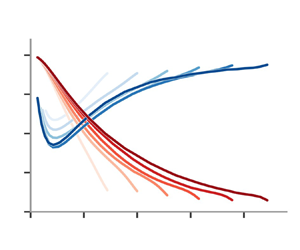
 \begin{equation} \varPi^{v}\approx{-}\varepsilon^{v} (1 - A (r/y)^{2/3} -B(r/\eta)^{{-}4/3}), \end{equation}
where we now omit superscripts for ease of notation.
This last equation has the following two verifiable implications, both of which are relatively easy to verify with the DNS data at our disposal. First, it implies that the value of  $r$ where
  $\varPi ^{v}/\varepsilon ^{v}$ is minimal and closest to the Kolmogorov equilibrium value
  $-1$ is
 \begin{equation} r_{min} \sim \sqrt{\delta_{\nu} y} \sim \lambda \end{equation}
based on the definition  $\lambda ^{2}\equiv 10\nu K/\varepsilon$ (already used by Dallas et al. (Reference Dallas, Vassilicos and Hewitt2009) in the context of FD TCF), and on
  $K\sim u_{\tau }^{2}$ and
  $\varepsilon \sim u_{\tau }^{3}/y$ being good enough approximations in the present context for
  $\delta _{\nu }\ll y \ll \delta$. Conclusions such as (6.19) and (6.20) have recently been obtained by Zimmerman et al. (Reference Zimmerman, Antonia, Djenidi, Philip and Klewicki2022) for the centreline of FD TCF and central axis of turbulent pipe flow where turbulence production is effectively absent.
Second, (6.19) also implies that the value  $(\varPi ^{v}/\varepsilon ^{v})_{min}$ of
  $\varPi ^{v}/\varepsilon ^{v}$ at
  $r=r_{min}$ obeys
 \begin{equation} 1+(\varPi^{v}/\varepsilon^{v})_{min} \sim y^{+^{{-}1/3}}\sim Re_{\lambda}^{{-}2/3}, \end{equation}
where  $Re_{\lambda } = \sqrt {K}\lambda /\nu$. Consistent with our averages over spheres in
  $\boldsymbol {r}$-space, these definitions of
  $\lambda$ and
  $Re_{\lambda }$ ignore some anisotropies of FD TCF. It is possible to define different Taylor lengths for different directions so as to take explicit account of anisotropies, which is an approach we have taken in another study (Yuvaraj Reference Yuvaraj2022). It may be noteworthy that the Corrsin length (Sagaut & Cambon Reference Sagaut and Cambon2018) does not appear spontaneously from our analysis, whereas the Kolmogorov and Taylor lengths do. The reason for this absence of the Corrsin length is that it equals
  $\kappa y$ at the approximation level of our theory in the intermediate layer
  $\delta _{\nu }\ll y \ll \delta$ and is therefore comparable to the outer bound of the range
  $r\le 2y$ considered here.
In conclusion, the non-homogeneous but statistically stationary case of FD TCF in the intermediate layer  $\delta _{\nu }\ll y \ll \delta$ is such that Kolmogorov equilibrium is achieved asymptotically around
  $\lambda$ and therefore not quite in an inertial range given that
  $\lambda$ depends on viscosity, and that there is a systematic departure from equilibrium when moving away from
  $\lambda$, both towards
  $L$ and towards
  $\eta$, see (6.19). (Note, however, that the non-zero deviation from Kolmogorov equilibrium as Reynolds number tends to infinity for a fixed small value of
  $r/y$ or for a fixed large value of
  $r/\eta$ (necessarily smaller than
  $\lambda /\eta$ in the limit) is small.) This is the same conclusion that the analysis of Lundgren (Reference Lundgren2002) reached for freely decaying, i.e. non-stationary, but statistically homogeneous and isotropic turbulence far from initial conditions. Two-point turbulence production (which increases with
  $r$ as confirmed in the following section) and its variation with wall-normal distance play a similar role in FD TCF as the rate of decay of the second-order velocity structure function (which increases with
  $r$ because unsteadiness increases with
  $r$) and its variation with time.
7. Comparison with DNS data for FD TCF
In this section, we compare the theory of the previous sections with the DNS data described in § 3.
In figure 5(a,b), we plot the two-point turbulence production rate  $\mathcal {P}^{v}$ and the interscale transfer rate
  $\varPi ^{v}$, both normalised by the turbulence dissipation rate
  $\varepsilon ^{v}$. We plot them vs
  $r/\lambda$ because of our prediction that the value of
  $r$, where
  $\varPi ^{v}/\varepsilon ^{v}$ is minimal, scales with
  $\lambda$. The maximum values of
  $r$ in the plots are bounded by
  $2y$ because of wall-blocking. We see that the normalised two-point turbulence production rate
  $\mathcal {P}^{v}/\varepsilon ^{v}$ increases from close to
  $0$ to a little under 1 as
  $r$ increases from
  $0$ to
  $2y$. This is evidenced for a wide range of wall-normal distances
  $y$ and for both Reynolds numbers at our disposal. It makes sense that the two-point turbulence production acts as a generation of turbulent kinetic energy at the larger
  $r$ scales but decreasingly so at smaller and smaller scales till it vanishes at the very smallest ones.

Figure 5. Interscale transfer rate  $\varPi$ (blue lines) and production rate
  $\mathcal {P}$ (red lines), integrated over the volume of sphere with radius
  $r$, normalised by the volume integral of the two-point dissipation rate
  $\varepsilon$ as a function of
  $r/\lambda$. Wall-normal distance is increased from light to dark colours. (a) For
  $Re_\tau =932$ and (b) for
  $Re_\tau =2003$.
It is also clear from figure 5(a,b) that  $\varPi ^{v}$ is negative for all scales and wall distances, indicating a forward, on average, energy cascade for
  $r < 2y$. Furthermore,
  $\varPi ^{v}/\varepsilon ^{v}$ has a minimum at
  $r_{min}$ close to
  $\lambda$ for a wide range of
  $y$ within
  $\delta _{\nu }\ll y \ll \delta$ and for both Reynolds numbers. This confirms our prediction (6.20) as can be seen in figure 6(a) where we plot, in blue,
  $r_{min}/\lambda$ vs
  $y^{+}$ for both Reynolds numbers and find that
  $r_{min} \approx 1.2\lambda$. One also sees in figure 5(a,b) that
  $(\varPi ^{v}/\varepsilon ^{v})_{min}$ increases in magnitude with increasing
  $y^+$ and with increasing
  $Re_{\tau }$. This is confirmed in figure 6(b) where we plot, in blue,
  $1+ (\varPi ^{v}/\varepsilon ^{v})_{min}$ vs
  $Re_{\lambda }$ confirming that
  $-(\varPi ^{v}/\varepsilon ^{v})_{min}$ increases towards
  $1$ following our prediction 6.21, which collapses both the
  $y^{+}$ and the
  $Re_{\tau }$ dependencies of
  $-(\varPi ^{v}/\varepsilon ^{v})_{min}$. Note, in passing, that the values of
  $Re_{\lambda }$ are not so high for the present
  $Re_{\tau }$ values of approximately
  $1000$ to
  $2000$: they range from approximately
  $50$ to
  $120$ (and in fact reach no more than a maximum of
  $200$ at the outer edge of the intermediate
  $y$-range if
  $Re_{\tau }$ is pushed up to
  $5200$ as Apostolidis et al. Reference Apostolidis, Laval and Vassilicos2022 also found).

Figure 6. (a) Values of  $r/\lambda$ where minima of
  $\varPi ^{v}/\varepsilon ^{v}$ are observed as a function of wall distance
  $y^+$. (b) Values of
  $1+(\varPi ^{v}/\varepsilon ^{v})_{min}$, in blue, as a function of
  $Re_\lambda$. Dashed line shows a scaling of
  $Re_\lambda ^{-2/3}$. Circle markers for
  $Re_\tau =932$; square markers for
  $Re_\tau =2003$.
The imbalance seen in figure 5 between  $\varPi ^{v}$ and
  $\varepsilon ^{v}$ is a clear indication that other processes in the scale-by-scale energy budget are active. The theoretical arguments of §§ 6.1 and 6.2 concluded that the scale-by-scale balance is approximately
  $\varPi ^{v}-\mathcal {P}^{v}\approx -\varepsilon ^{v}$ at the outer scales and
  $\varPi ^{v}-D_{r}^{v}\approx -\varepsilon ^{v}$ at the inner scales. This prediction is made in the limit
  $Re_{\tau }=\delta /\delta _{\nu } \gg 1$ and
  $\delta _{\nu }\ll y \ll \delta$ and, as the values of
  $Re_{\lambda }$ suggest, the Reynolds numbers in the DNS data we are using may not be high enough. Nevertheless, figure 7(a,b) does reveal some tendency for
  $(\varPi ^{v}-\mathcal {P}^{v})/\varepsilon ^{v}$ to collapse as a function of
  $r/y$ and tend towards
  $-1$ at the higher values of
  $r/y$ as
  $y^{+}$ grows, in particular for the higher of our two Reynolds numbers
  $Re_{\tau }$. Furthermore, figure 7(c,d) reveals some tendency for
  $(\varPi ^{v}-D_{r}^{v})/\varepsilon ^{v}$ to collapse as a function of
  $r/\eta$ as
  $y^{+}$ grows and even to tend towards
  $-1$ at the smallest values of
  $r/\eta$.

Figure 7. (a,b) ( $\varPi ^{v}-\mathcal {P}^{v})/\varepsilon ^{v}$ as a function of
  $r/y$: (a) for
  $Re_\tau =932$ and (b) for
  $Re_\tau =2003$. (c,d)
  $(\varPi ^{v}-D^{v})/\varepsilon ^{v}$ as a function of
  $r/\eta$: (c) for
  $Re_\tau =932$ and (d) for
  $Re_\tau =2003$. Wall-normal distance is increased from light to dark colours.
Finally, we compare the high-Reynolds-number predictions (6.15), (6.16) and (6.19) with the DNS data. In figure 8(a,b), we plot  $S_{2}/u_{\tau }^{2}(r/y)^{2/3}$ and
  $S_{12}/u_{\tau }^{2}(r/y)^{2/3}$ vs
  $r/y$ to test outer scalings and in figure 8(c,d), we plot the same quantities vs
  $r/\eta$ to test inner scalings. Note that we use
  $u_{\tau }^{3}/y$ as an estimate of
  $\varepsilon ^{v}$. Our DNS data lend more support to our
  $r^{2/3}$ prediction for
  $S_{12}$ than for
  $S_2$, and a better outer collapse in terms of
  $r/y$ of
  $S_{12}/u_{\tau }^{2}(r/y)^{2/3}$ than
  $S_{2}/u_{\tau }^{2}(r/y)^{2/3}$. However, the inner collapse in terms of
  $r/\eta$ appears better for
  $S_{2}/u_{\tau }^{2}(r/y)^{2/3}$ than
  $S_{12}/u_{\tau }^{2}(r/y)^{2/3}$. At any rate, the values of
  $Re_{\lambda }$ are quite low in the DNS data used here for a conclusive comparison between these data and theoretical predictions made in the double limit
  $Re_{\tau }\to \infty$,
  $y^{+} \to \infty$ (i.e.
  $Re_{\lambda }\sim \lambda /\delta _{\nu }\sim (y^{+})^{1/2}\to \infty$) with the constraint
  $y\ll \delta$. In fact, even at the very lowest/leading order, our predictions (6.15), (6.16) are incomplete as they should have corrections in terms of powers of
  $r/\eta$ and
  $r/y$ which are beyond the present theory and which surely matter in comparisons with DNS data.

Figure 8.  $S_{12}$ in orange colours (multiplied by a factor of 3 for ease of comparison) and
  $S_{2}$ in marine colours normalised with
  $u_\tau ^{2}(r/y)^{2/3}$ as a function of (a,b)
  $r/y$ and of (c,d)
  $r/\eta$: (a,c) for
  $Re_\tau =932$; (b,d) for
  $Re_\tau =2003$. Wall-normal distance is increased from light to dark colours.
We close this section with a comparison in figure 9 of (6.19) with the DNS data which is clearly better for  $Re_{\tau } = 2003$ than
  $Re_{\tau }=932$.

Figure 9. Rearrangement of (6.19) vs  $r/y$: (a) for
  $Re_\tau =932$; (b) for
  $Re_\tau =2003$. Wall-normal distance is increased from light to dark colours.
8. Interscale transfer decompositions
The two main conclusions of the previous sections concern (i) the importance of the Taylor length in defining the scale where the normalised interscale transfer rate  $\varPi ^{v}/\varepsilon ^{v}$ has a minimum and is closest to the equilibrium value
  $\varPi ^{v}/\varepsilon ^{v}=-1$ and (ii) the importance of sweeps and ejections but also of aligned and anti-aligned pairs of fluctuating velocities in determining the sign and magnitude of the two-point turbulence production rate
  $\mathcal {P}^{v}$. Looking at (4.2), we start this section by asking whether aligned and anti-aligned pairs of fluctuating velocities also directly affect the interscale transfer rate
  $\varPi ^{v}$.
8.1. Aligned/anti-aligned decomposition
Equation (4.2) shows that a scale-space flux and a cascade from large to small or from small to large scales correspond to a negative or positive  $({3}/{4{\rm \pi} })\int \langle ({\hat {\boldsymbol {r}} \boldsymbol {\cdot } \delta \boldsymbol {u}}/{r}) \vert \delta \boldsymbol {u}\vert ^{2}\rangle \,{\rm d}\varOmega _{\boldsymbol {r}}$ and contributes a growth or decrease of TKE at scales
  $r$ and smaller (see Chen & Vassilicos Reference Chen and Vassilicos2022). Local compression, i.e.
  $\delta \boldsymbol {u} \boldsymbol {\cdot } \hat {r} < 0$, causes local forward cascade and local stretching, i.e.
  $\delta \boldsymbol {u} \boldsymbol {\cdot } \hat {r} > 0$, causes local inverse cascade. Our observation that
  $\varPi ^{v}$ is negative at all scales means that local compressions prevail at all scales, but are they mostly caused by aligned or anti-aligned pairs of fluctuating velocities? This question introduces our first decomposition, namely
 \begin{equation} \varPi^{v} = \varPi^{v}_{\rightrightarrows} + \varPi^{v}_{\rightleftarrows}= \frac{3}{4 {\rm \pi}} \int \left\langle \frac{\delta \boldsymbol{u}\boldsymbol{\cdot} \hat{\boldsymbol{r}}}{r}\vert \delta \boldsymbol{u}\vert^2\right\rangle_{\rightrightarrows} \,{\rm d}\varOmega_{r} + \frac{3}{4 {\rm \pi}} \int \left\langle \frac{\delta \boldsymbol{u}\boldsymbol{\cdot} \hat{\boldsymbol{r}}}{r}\vert \delta \boldsymbol{u}\vert^2\right\rangle_{\rightleftarrows}\,{\rm d}\varOmega_{r}, \end{equation}
where  $\varPi ^{v}_{\rightrightarrows }$ and
  $\varPi ^{v}_{\rightleftarrows }$ are respectively equal to the first and second terms on the left-hand side which are calculated using averages
  $\langle \cdots \rangle _{\rightrightarrows }$ conditional on
  $\boldsymbol {u}^+ \boldsymbol {\cdot } \boldsymbol {u}^{-}>0$ and averages
  $\langle \cdots \rangle _{\rightleftarrows }$ conditional on
  $\boldsymbol {u}^+ \boldsymbol {\cdot }\boldsymbol {u}^{-}<0$.
Compressive and stretching relative motions may not balance in terms of energy transfer, resulting in a non-vanishing  $\varPi ^{v}$, but they do balance in terms of mass transfer because of incompressibility which implies
  $\int \delta \boldsymbol {u} \boldsymbol {\cdot } \hat {r}\,{\rm d}\varOmega _{r} =0$. Hence,
 \begin{equation} \int \langle \delta \boldsymbol{u}\boldsymbol{\cdot}\hat{\boldsymbol{r}}\rangle_{\rightrightarrows} \,{\rm d}\varOmega_{r} + \int \langle \delta \boldsymbol{u}\boldsymbol{\cdot}\hat{\boldsymbol{r}}\rangle_{\rightleftarrows} \,{\rm d}\varOmega_{r}=0. \end{equation}
In figure 10, we plot both terms on the left-hand side of this equation as functions of  $r$ for various wall distances
  $y$. We also plot
  $\int \delta \boldsymbol {u} \boldsymbol {\cdot } \hat {r} \,{\rm d}\varOmega _{r}$ for comparison and as a check that it is indeed zero in the DNS irrespective of
  $r$ and
  $y$. The first observation is that aligned fluctuation pairs are stretching relative motions on average given the positive sign of
  $\int \langle \delta \boldsymbol {u}\boldsymbol {\cdot } \hat {\boldsymbol {r}}\rangle _{\rightrightarrows } \,{\rm d}\varOmega _{r}$. The joint PDFs of figure 11 show that relative motions of aligned fluctuation pairs are stretching as a result of
  $\delta \boldsymbol {u}$ having a tendency to be directed in the same direction as the separation vector
  $\boldsymbol {r}$ for pairs of aligned fluctuating velocities. This tendency weakens with increasing
  $r$ irrespective of wall distance
  $y$ and, consistently,
  $\int \langle \delta \boldsymbol {u}\boldsymbol {\cdot } \hat {\boldsymbol {r}}\rangle _{\rightrightarrows } \,{\rm d}\varOmega _{r}$ tends to
  $0$ with increasing
  $r$.
$r$.

Figure 10.  $\int \langle \delta \boldsymbol {u}\boldsymbol {\cdot } \hat {\boldsymbol {r}}\rangle {\rm d}\varOmega _{r}$ integrated over the whole sphere in black lines, conditionally integrated over anti-aligned pairs in marine colours, and conditionally integrated over aligned pairs in orange colours. Wall-normal distance is increased from light to dark colours. (a)
  $Re_\tau =932$, (b)
  $Re_\tau =2003$. (c)
  $r/\lambda$ positions of the minima/maxima observed in panel (a) as a function of wall-distance
  $y^+$ for
  $Re_\tau =932$, similarly in panel (d) for
  $Re_\tau =2003$.

Figure 11. Joint probability distribution functions (JPDFs) of  $\delta \boldsymbol {u}\boldsymbol {\cdot }\boldsymbol {\hat {r}}/|\delta \boldsymbol {u}|$ and
  $\boldsymbol {u}^{-}\boldsymbol {u}^{+}/\sqrt {|\boldsymbol {u}^{+}|^2|\boldsymbol {u}^{-}|^2}$. (a) For
  $Re_\tau =932$ and wall-distance
  $y^+=257$, four different JPDFs with increasing scale
  $r/\lambda =0.38,0.57,1.05$ and
  $2.91$. (b) Similarly for
  $Re_\tau =2003$ and wall-distance
  $y^+=456$, the JPDFs correspond to scales
  $r/\lambda =0.35,0.56,1.10$ and
  $3.43$. The joint PDFs are normalised with their maximum value. Above each JPDF, we also plot the conditional PDF of
  $\delta \boldsymbol {u}\boldsymbol {\cdot }\boldsymbol {\hat {r}}/|\delta \boldsymbol {u}|$, conditioned on aligned (red lines) and anti-aligned (blue lines) pairs.
The second observation in figure 10 is that anti-aligned fluctuation pairs are compressing relative motions, on average, given the negative sign of  $\int \langle \delta \boldsymbol {u}\boldsymbol {\cdot } \hat {\boldsymbol {r}}\rangle _{\rightleftarrows }\,{\rm d}\varOmega _{r}$. Looking at figure 11, it does not seem possible to explain this behaviour purely in terms of velocity directions. However, the joint PDFs of figure 12 reveal that the range of values over which
  $\delta \boldsymbol {u}\boldsymbol {\cdot } \hat {\boldsymbol {r}}$ fluctuates around zero is much wider for anti-aligned than for aligned fluctuations. This effect has to do with the intensity of the fluctuating velocities, not only their relative directions. This very wide fluctuation range is slightly skewed towards negative values of
  $\delta \boldsymbol {u}\boldsymbol {\cdot } \hat {\boldsymbol {r}}$ for pairs of fluctuating velocities which are anti-aligned, thereby accounting for the compressive average behaviour of anti-aligned pairs (
 $\boldsymbol {u}^+ \boldsymbol {\cdot } \boldsymbol {u}^{-}<0$). This skewness diminishes with increasing
  $r$ irrespective of wall distance
  $y$ and, consistently,
  $\int \langle \delta \boldsymbol {u}\boldsymbol {\cdot } \hat {\boldsymbol {r}}\rangle _{\rightleftarrows } \,{\rm d}\varOmega _{r}$ tends to
  $0$ with increasing
  $r$. Note, finally, that it is far more likely to find aligned (
 $\boldsymbol {u}^+ \boldsymbol {\cdot } \boldsymbol {u}^{-}>0$) than anti-aligned (
 $\boldsymbol {u}^+ \boldsymbol {\cdot } \boldsymbol {u}^{-}<0$) pairs as figure 11 shows.

Figure 12. Joint probability distribution functions (JPDFs) of  $\delta \boldsymbol {u}\boldsymbol {\cdot }\boldsymbol {\hat {r}}$ and
  $\boldsymbol {u}^{-}\boldsymbol {u}^{+}$. (a) For
  $Re_\tau =932$ and wall-distance
  $y^+=257$, four different JPDFs with increasing scale
  $r/\lambda =0.38,0.57,1.05$ and
  $2.91$. (b) Similarly for
  $Re_\tau =2003$ and wall-distance
  $y^+=456$, the JPDFs correspond to scales
  $r/\lambda =0.35,0.56,1.10$ and
  $3.43$. The joint PDFs are normalised with their maximum value, while the values of the
  $x$ and
  $y$ axis are normalised with their own standard deviations.
The third observation in figure 10 is that  $\int \langle \delta \boldsymbol {u}\boldsymbol {\cdot } \hat {\boldsymbol {r}}\rangle _{\rightleftarrows } \,{\rm d}\varOmega _{r}$ has a minimum at
  $r=r_m$ near
  $r_{min}\approx 1.2\lambda$ for all
  $y$ and that
  $\int \langle \delta \boldsymbol {u}\boldsymbol {\cdot } \hat {\boldsymbol {r}}\rangle _{\rightrightarrows } \,{\rm d}\varOmega _{r}$ has a maximum at the same value
  $r=r_m$ for all
  $y$. As seen in the previous two sections,
  $r_{min}$ is the value of
  $r$ where
  $\varPi ^{v}/\varepsilon ^{v}$ has its minimum. In figure 10(c,d), we plot the positions
  $r$ of the maxima and minima in figure 10 vs wall distance for both DNS Reynolds numbers at our disposal. It is quite striking that, for all wall distances and both Reynolds numbers tried,
  $\int \langle \delta \boldsymbol {u}\boldsymbol {\cdot } \hat {\boldsymbol {r}}\rangle _{\rightleftarrows }\,{\rm d}\varOmega _{r}$ and
  $\int \langle \delta \boldsymbol {u}\boldsymbol {\cdot } \hat {\boldsymbol {r}}\rangle _{\rightrightarrows }\,{\rm d}\varOmega _{r}$ peak at
  $r=r_m$ close to the value
  $r=r_{min}$, where
  $\varPi ^{v}/\varepsilon ^{v}$ peaks and is closest to the equilibrium
  $-1$ value. Even though
  $r_m$ drifts slightly from
  $r_{min}\approx 1.2\lambda$ at relatively high wall-normal distances, the suggestion is that, in the layer
  $\delta _{\nu }\ll y \ll \delta$ of FD TCF, Kolmogorov-like equilibrium may be achieved at those length scales
  $r$ where aligned fluctuating velocities are stretching with their difference
  $\delta \boldsymbol {u}$ maximally or near-maximally aligned with the separation vector
  $\boldsymbol {r}$ and where anti-aligned fluctuations are maximally or near-maximally skewed towards large negative values of
  $\delta \boldsymbol {u}\boldsymbol {\cdot } \hat {\boldsymbol {r}}$. This is a conclusion that is well beyond the reach of the theory in § 6 but which we might not have been able to reach without it. (We refer to Kolmogorov-like rather than Kolmogorov equilibrium because the scale
  $r_{min}$ is proportional to the Taylor scale and therefore depends on viscosity.)
It is shown in § 5 that anti-aligned fluctuation pairs enhance the positive two-point turbulence production rate in the layer  $\delta _{\nu }\ll y \ll \delta$ of FD TCF: we have now seen that these anti-aligned fluctuation pairs are, on average, compressive and figure 13 shows that
  $\varPi ^{v}_{\rightleftarrows }$ is consistently negative, indicating forward cascade. Therefore, anti-aligned fluctuations do not only enhance the two-point production rate at all
  $r$, they also contribute a forward cascade at all
  $r$ in the layer
  $\delta _{\nu }\ll y \ll \delta$ of FD TCF. Note, however, that the minimum value of
  $\varPi ^{v}_{\rightleftarrows }$ is not at
  $r=r_{min}$, where
  $\varPi ^{v}/\varepsilon ^{v}$ has its minimum value and is closest to the equilibrium
  $-1$ value. In fact, the
  $r$-position of the minimum value of
  $\varPi ^{v}_{\rightleftarrows }$ does not scale with
  $\lambda$. The scaling of
  $r_{min}$ therefore requires taking into account both aligned and anti-aligned fluctuations.

Figure 13. Decomposition of the interscale transfer term  $\varPi ^{v}$ (black lines) into
  $\varPi ^{v}_{\rightleftarrows }$ (blue lines) and
  $\varPi ^{v}_{\rightrightarrows }$ (red lines): (a)
  $Re_\tau =932$; (b)
  $Re_\tau =2003$. Wall-normal distance is increased from light to dark colours.
Aligned fluctuation pairs impose a loss of energy on scales smaller than  $r$ by mean flow interaction with turbulence fluctuations and thereby reduce the one-point effect of sweeps and ejections on the two-point turbulence production rate (see § 5). We have now seen that aligned fluctuation pairs are on average stretching, which would suggest the presence of an average inverse cascade element to the interscale transfer rate
  $\varPi ^{v}_{\rightrightarrows }$. Figure 13 shows that
  $\varPi ^{v}_{\rightrightarrows }$ is positive (though only slightly so), and an average inverse cascade by aligned fluctuations is indeed present at scales
  $r$ larger than approximately 2 to 3 times
  $\lambda$ for the Reynolds numbers of the DNS data used here. However, figure 13 also shows that
  $\varPi ^{v}_{\rightrightarrows }$ is negative at smaller scales. Stretching aligned fluctuating motions at scales of the order of the Taylor length and below may dominate over compressive aligned fluctuating motions, on average, but they do not dominate interscale energy transfer at these scales. There is no contradiction with the positive values of
  $\int \langle \delta \boldsymbol {u}\boldsymbol {\cdot } \hat {\boldsymbol {r}}\rangle _{\rightrightarrows }\,{\rm d}\varOmega _{r}$ in figure 10. The different signs of this solid angle integral and the solid angle integral in the definition of
  $\varPi ^{v}_{\rightrightarrows }$ (see (8.1)) are an effect of small-scale anisotropies over which we are averaging. Future studies of interscale transfers in FD TCFs will need to take these anisotropies into account for a finer description of the physics.
Finally, comparing the plots of  $\varPi ^{v}$ in figure 5 with those of
  $\varPi ^{v}_{\rightrightarrows }$ and
  $\varPi ^{v}_{\rightleftarrows }$ in figure 13 shows that
  $\varPi ^{v}_{\rightleftarrows }$ dominates over
  $\varPi ^{v}_{\rightrightarrows }$ at scales of the order of
  $\lambda$ and larger, and is mostly responsible for the value of
  $\varPi ^{v}$. At smaller scales, however,
  $\varPi ^{v}_{\rightrightarrows }$ becomes equally important and of the same negative sign as
  $\varPi ^{v}_{\rightleftarrows }$ so that the actual negative value of
  $\varPi ^{v}$ cannot be accounted for by only one or the other: the interscale turbulence energy transfers of both aligned and anti-aligned fluctuations matter.
8.2. Homogeneous/Inhomogeneous energy transfer decomposition
As already mentioned at the start of § 8.1, the right-hand side  $({3}/{4{\rm \pi} })\int \langle ({\hat {\boldsymbol {r}} \boldsymbol {\cdot } \delta \boldsymbol {u}}/{r}) \vert \delta \boldsymbol {u}\vert ^{2}\rangle {\rm d}\varOmega _{\boldsymbol {r}}$ of (4.2) shows that local compression, i.e.
  $\delta \boldsymbol {u} \boldsymbol {\cdot } \hat {r} < 0$, causes local forward cascade, whereas local stretching, i.e.
  $\delta \boldsymbol {u}\boldsymbol {\cdot } \hat {r} > 0$, causes local inverse cascade (see also § 2 of Chen & Vassilicos Reference Chen and Vassilicos2022). These compressions and stretches may be caused either by turbulence inhomogeneities or by correlated ‘eddy’ motions. In an attempt to formalise this distinction, Alves Portela, Papadakis & Vassilicos (Reference Alves Portela, Papadakis and Vassilicos2020) decomposed the interscale energy transfer rate
  $\varPi = ({\partial }/{\partial r_i}) ( \delta u_i |\delta \boldsymbol {u}|^2 )$ as follows:
 \begin{equation}
\frac{\partial}{\partial r_i} (\delta u_i |\delta
\boldsymbol{u}|^2) = \frac{\partial}{\partial r_i}
[\delta u_i(|\boldsymbol{u}^+|^2+|\boldsymbol{u}^-|^2)]
-2\frac{\partial}{\partial r_i}(\delta u_i \boldsymbol{u}^- \boldsymbol{\cdot} \boldsymbol{u}^+),
\end{equation}
\begin{equation}
\frac{\partial}{\partial r_i} (\delta u_i |\delta
\boldsymbol{u}|^2) = \frac{\partial}{\partial r_i}
[\delta u_i(|\boldsymbol{u}^+|^2+|\boldsymbol{u}^-|^2)]
-2\frac{\partial}{\partial r_i}(\delta u_i \boldsymbol{u}^- \boldsymbol{\cdot} \boldsymbol{u}^+),
\end{equation}
where the first term on the right-hand side can be rigorously recast into a gradient in centroid  $\boldsymbol {x}$-space leading to
 \begin{align} \frac{\partial}{\partial
r_i} (\delta u_i |\delta \boldsymbol{u}|^2) &=
\frac{1}{2}\frac{\partial}{\partial x_i}[ u_i^+
|\boldsymbol{u}^+|^2 + u_i^- |\boldsymbol{u}^-|^2 - u_i^-
|\boldsymbol{u}^+|^2 - u_i^+|\boldsymbol{u}^-|^2]
\nonumber\\ &\quad -2\frac{\partial}{\partial
r_i}(\delta u_i \boldsymbol{u}^- \boldsymbol{\cdot}\boldsymbol{u}^+).
\end{align}
\begin{align} \frac{\partial}{\partial
r_i} (\delta u_i |\delta \boldsymbol{u}|^2) &=
\frac{1}{2}\frac{\partial}{\partial x_i}[ u_i^+
|\boldsymbol{u}^+|^2 + u_i^- |\boldsymbol{u}^-|^2 - u_i^-
|\boldsymbol{u}^+|^2 - u_i^+|\boldsymbol{u}^-|^2]
\nonumber\\ &\quad -2\frac{\partial}{\partial
r_i}(\delta u_i \boldsymbol{u}^- \boldsymbol{\cdot}\boldsymbol{u}^+).
\end{align}
Here,  $\varPi _I \equiv \frac {1}{2}({\partial }/{\partial x_i})[ u_i^+ |\boldsymbol {u}^+|^2 + u_i^- |\boldsymbol {u}^-|^2 - u_i^- |\boldsymbol {u}^+|^2 - u_i^+ |\boldsymbol {u}^-|^2 ]$ is interpreted as an inhomogeneity-related interscale turbulent energy transfer rate. In statistically homogeneous turbulence, the average
  $\langle \varPi _I \rangle$ is indeed zero and the interscale turbulent energy transfer rate is only accountable to
  $\varPi _{H}\equiv -2({\partial }/{\partial r_i})(\delta u_i \boldsymbol {u}^- \boldsymbol {\cdot } \boldsymbol {u}^+)$ on average.
Integrating  $\varPi$,
  $\varPi _{I}$ and
  $\varPi _H$ over the sphere of radius
  $r$ in
  $\boldsymbol {r}$-space to obtain
  $\varPi ^v$,
  $\varPi _{I}^v$ and
  $\varPi _{H}^{v}$, respectively, and then applying the Gauss divergence theorem, we obtain
 \begin{align} \varPi^{v} = \varPi_I^{v} + \varPi_H^{v} &= \frac{3}{4{\rm \pi}} \left(\int\left\langle\frac{\delta \boldsymbol{u} \boldsymbol{\cdot} \hat{\boldsymbol{r}}}{r}(|\boldsymbol{u}^+|^2 + |\boldsymbol{u}^-|^2) \right\rangle \,{\rm d} \varOmega_r \right. \nonumber\\ &\quad \left.- 2\int\left\langle\frac{\delta \boldsymbol{u} \boldsymbol{\cdot} \hat{\boldsymbol{r}}}{r}(\boldsymbol{u}^- \boldsymbol{\cdot} \boldsymbol{u}^+) \right\rangle \,{\rm d} \varOmega_r \right). \end{align}
This decomposition is partly related to that in § 8.1 because  $\varPi _H^{v}$ is linearly dependent on correlations between
  $\delta \boldsymbol {u} \boldsymbol {\cdot } \hat {r}$ and
  $\boldsymbol {u}^- \boldsymbol {\cdot } \boldsymbol {u}^+$, and the sign of
  $\boldsymbol {u}^- \boldsymbol {\cdot } \boldsymbol {u}^+$ indicates whether velocity fluctuation pairs are aligned or anti-aligned, which is the basis of decomposition (8.1). Whilst it follows immediately from (8.4) that
  $\varPi _I^{v} =0$ if the term inside the
  $\boldsymbol {x}$-gradient in that equation is statistically homogeneous, (8.5) shows that
  $\varPi _I^{v}=0$ if
  $\delta \boldsymbol {u} \boldsymbol {\cdot } \hat {\boldsymbol {r}}$ and
  $(|\boldsymbol {u}^+|^2 + |\boldsymbol {u}^-|^2)$ are uncorrelated and if
  $(|\boldsymbol {u}^+|^2 + |\boldsymbol {u}^-|^2)$ is statistically homogeneous. Of course, this is not the only and necessary way for
  $\varPi _I^{v}$ to vanish. In particular, there may be cases of non-homogeneity for which
  $\varPi _I^{v}$ vanishes too, for example, cases where
  $\varPi _I^{v}$ vanishes but
  $\varPi _I$ does not.
In figure 14, we plot the terms  $\varPi _{I}^{v}$ and
  $\varPi _{H}^{v}$ in 8.5 normalised by the volume integral of the dissipation. For both Reynolds numbers, we observe that
  $\varPi _{H}^{v}$ dominates and describes almost perfectly the full interscale transfer
  $\varPi ^{v}$ for all scales
  $r \le 2y$ in the intermediate range of the channel (
 $y$ between multiples of
  $\delta _{\nu }$ and approximately half
  $\delta$). The average interscale transfer from large to small scales is nearly fully described by the negative value of
  $\varPi _{H}^{v}$ and the inhomogeneity-related interscale transfer rate
  $\varPi _{I}^{v}$ is close to zero. In a different non-homogenous turbulent flow, the turbulent wake of a square prism, Alves Portela et al. (Reference Alves Portela, Papadakis and Vassilicos2020) found a significant contribution of the inhomogeneity-related interscale transfer rate to the total interscale transfer rate. It is therefore not trivial that in FD TCF,
  $\varPi _{I}^{v}$ is negligible compared to
  $\varPi _{H}^{v}$ in spite of the statistical non-homogeneity of the FD TCF. However, this is partly an artefact of the integration over spheres in
  $\boldsymbol {r}$-space which we apply to
  $\varPi _{I}$ to obtain
  $\varPi _{I}^{v}$. If we lift this integration and use the DNS data to compute
  $\varPi _{I} (y, r_{1}, r_{2}, r_{3})$ as a function of
  $r_{2}/y$ for various values of wall-normal distance
  $y$ and various values of
  $r_1$ and
  $r_3$, we find (figure 15) that
  $\varPi _{I} (y, r_{1}, r_{2}, r_{3})$ is close to
  $0$ and negligible in most cases except for ‘attached eddies’, i.e. for values of
  $r_2$ relatively close to
  $2y$ (wall blocking implies
  $r_{2}\le 2y$) where it is positive, thereby potentially reflecting interscale transfer from small to large scales (similarly to Cimarelli et al. Reference Cimarelli, De Angelis, Jimenez and Casciola2016; Cho, Hwang & Choi Reference Cho, Hwang and Choi2018) except for
  $r_2$ near-equal to
  $2y$ where it is negative. The non-vanishing inhomogeneity-related interscale transfer of ‘attached eddies’ is averaged out when we integrate
  $\varPi _{I}$ to obtain
  $\varPi _{I}^{v}$.

Figure 14. Interscale transfer rate (blue lines), inhomogeneous part  $\varPi _I^{v}$ (red lines) and homogeneous part
  $\varPi _H^{v}$ (green lines), all integrated over the volume of a sphere and normalised by the dissipation rate integrated over the volume of the sphere as a function of
  $r/\lambda$. Wall-normal distance is increased from light to dark colours. (a) For
  $Re_\tau =932$ and (b) for
  $Re_\tau =2003$.

Figure 15.  $\varPi$ (blue markers),
  $\varPi _I$ (red lines) and
  $\varPi _H$ (green lines) normalised with the two-point dissipation rate
  $\varepsilon$ vs the wall-normal scale
  $r_2$ divided with
  $y$. (a)
  $Re_\tau =932$, from left to right we increase the streamwise scale
  $r_1$ and from top to bottom the spanwise scale
  $r_3$. (b) Similarly for
  $Re_\tau =2003$. Wall-normal distance is increased from light to dark colours.
Returning to  $\varPi _{H}^{v}$ and the fact that it has very similar dependencies on
  $r$ and
  $y$ as
  $\varPi ^{v}$, we note, in particular, that
  $\varPi _{H}^{v}$ has a minimum at the near same
  $r\approx r_{min}$ where
  $\varPi ^v$ has a minimum, and even that the minimum value of
  $\varPi _{H}^{v}$ closely obeys the same relation (6.21) that
  $\varPi ^{v}_{min}$ obeys (see figure 16). As seen in § 6, the two-point separation scale
  $r=r_{min}$ demarcates between smaller values of
  $r$ where
  $\varPi ^{v}$ is balanced by dissipation and viscous diffusion and larger values of
  $r$ where
  $\varPi ^{v}$ is balanced by dissipation and two-point turbulence production. However, the theory of § 6, which is conclusive for
  $\varPi ^{v}$, has no say on
  $\varPi _{H}^{v}$ and can therefore not explain our observation that
  $\varPi _{H}^{v}$ behaves very much like
  $\varPi ^{v}$. We therefore adopt a different point of view from that in § 6 and look at PDFs of instantaneous (in time) and local (in
  $(x,z)$ planes) interscale transfer rates
  ${\rm \pi} ^{v} \equiv ({3}/{4 {\rm \pi}}) \int ({\delta \boldsymbol {u}\boldsymbol {\cdot } \hat {\boldsymbol {r}}}/{r})\vert \delta \boldsymbol {u}\vert ^2\,{\rm d}\varOmega _{r}$,
  ${\rm \pi} _{H}^{v}\equiv -({3}/{2{\rm \pi} }) \int ({\delta \boldsymbol {u} \boldsymbol {\cdot } \hat {\boldsymbol {r}}}/{r})(\boldsymbol {u}^- \boldsymbol {\cdot } \boldsymbol {u}^+) \,{\rm d} \varOmega _r$ and
  ${\rm \pi} _{I}^{v} \equiv ({3}/{4{\rm \pi} }) \int ({\delta \boldsymbol {u} \boldsymbol {\cdot } \hat {\boldsymbol {r}}}/{r})(|\boldsymbol {u}^+|^2 + |\boldsymbol {u}^-|^2) \,{\rm d} \varOmega _r$. Clearly,
  $\varPi ^{v} = \langle {\rm \pi}^{v} \rangle$,
  $\varPi _{H}^{v} = \langle {\rm \pi}_{H}^{v} \rangle$ and
  $\varPi _{I}^{v} = \langle {\rm \pi}_{I}^{v} \rangle$.

Figure 16. (a) Values of  $r/\lambda$ where minima of
  $\varPi ^{v}/\varepsilon ^{v}$ and minima of
  $\varPi _{H}^{v}/\varepsilon ^{v}$ are observed as functions of wall distance
  $y^+$. (b) Values of
  $1+(\varPi ^{v}/\varepsilon ^{v})_{min}$ (in blue) and of
  $1+(\varPi _{H}^{v}/\varepsilon ^{v})_{min}$ (in green), as functions of
  $Re_\lambda$. Dashed line shows a scaling of
  $Re_\lambda ^{-2/3}$. Circle markers for
  $Re_\tau =932$, square markers for
  $Re_\tau =2003$.
In figure 17, we plot examples of PDFs of  ${\rm \pi} ^{v}$,
  ${\rm \pi} _{H}^{v}$ and
  ${\rm \pi} _{I}^{v}$ for a couple of wall distances
  $y$ within the intermediate range
  $\delta _{\nu }\ll y\ll \delta$ and for different values of separation scale
  $r$ to see how these PDFs evolve with varying
  $r$. As pointed out by Alves Portela et al. (Reference Alves Portela, Papadakis and Vassilicos2020), at
  $r=0$, we have
  $\varPi ^{v}= \varPi _{H}^{v}=\varPi _{I}^{v}=0$. As
  $r$ progressively increases, the PDFs of
  ${\rm \pi} ^{v}$ and
  ${\rm \pi} _{H}^{v}$ move to the left towards increasingly negative values, as shown in the insets of figure 17(a,b,e, f). This overall PDF drift is most pronounced at the smaller values of
  $r$, and causes
  $\varPi ^{v}$ and
  $\varPi _{H}^{v}$ to progressively decrease below
  $0$ as
  $r$ increases. However, the skewnesses of the PDFs of
  ${\rm \pi} ^{v}$ and of
  ${\rm \pi} _{H}^{v}$ grow from negative values close to
  $-10$ at the smallest separations
  $r$ to values between
  $-1$ and even slightly positive as
  $r$ grows (see figure 18(a,b,e, f)). This evolution of the skewnesses of these two PDFs counteracts their overall drift towards increasingly negative values and acts to bring
  $\varPi ^{v}$ and
  $\varPi _{H}^{v}$ back towards zero as
  $r$ increases. The minima of
  $\varPi ^{v}$ and
  $\varPi _{H}^{v}$ occur as a result of these two counteracting tendencies, the overall drift dominating at scales
  $r$ smaller than
  $r_{min}$ and causing
  $\varPi ^{v}$ and
  $\varPi _{H}^{v}$ to decrease, and the decreasingly skewed PDF dominating at scales larger than
  $r_{min}$ and causing
  $\varPi ^{v}$ and
  $\varPi _{H}^{v}$ to increase.

Figure 17. Probability density functions (PDFs) of (a,b)  ${\rm \pi} ^{v}$, (c,d)
  ${\rm \pi} _I^{v}$ and (e, f)
  ${\rm \pi} _H^{v}$ normalised with their respective maximum probability. The values of the terms are normalised with their own standard deviation. The scale
  $r$ is increased from light to dark colours. (a,c,e)
  $Re_\tau =932$, (b,d, f)
  $Re_\tau =2003$. Inset is a zoom of the area close to the maximum probability in lin–lin axes.

Figure 18. Skewness factor of  ${\rm \pi} ^{v}$ in blue colours,
  ${\rm \pi} _I{^v}$ in red colours and of
  ${\rm \pi} _H^{v}$ in green colours as a function of
  $r/\lambda$, for different wall-normal locations. The wall-distance
  $y$ is increased from light to dark colours. (a) For
  $Re_\tau =932$ and (b) for
  $Re_\tau =2003$.
The PDF of the inhomogeneity-related interscale transfer rates  ${\rm \pi} _{I}^{v}$ is radically different as far as skewness is concerned (see figure 18). Whilst the PDFs of both
  ${\rm \pi} ^{v}$ and
  ${\rm \pi} _{H}^{v}$ are skewed towards forward cascade events at small
  $r$ and evolve with increasing
  $r$ towards not being skewed or even being slightly skewed towards inverse cascade events, the PDF of
  ${\rm \pi} _{I}^{v}$ is highly skewed towards inverse cascade events at small
  $r$ and evolves very quickly with increasing
  $r$ towards not being very skewed. It remains only slightly skewed (positively or negatively) for all permissible
  $r$ larger than approximately
  $2\lambda$ (the word ‘permissible’ refers to
  $r\le 2y$). The difference is not only that the PDF of
  ${\rm \pi} _{I}^{v}$ is oppositely skewed to the PDFs of
  ${\rm \pi} ^{v}$ and
  ${\rm \pi} _{H}^{v}$ at small
  $r$, but the equally if not even more important difference is that, as
  $r$ increases, the skewness of
  ${\rm \pi} _{I}^{v}$ evolves much faster towards small absolute values (which it actually reaches at
  $r\approx 2\lambda$) than the skewnesses of
  ${\rm \pi} _{H}^{v}$ and
  ${\rm \pi} ^v$ which evolve much more gradually towards values around and larger than
  $-1$.
$-1$.
However, the PDF of  ${\rm \pi} _{I}^{v}$ is similar to the PDFs of
  ${\rm \pi} ^{v}$ and
  ${\rm \pi} _{H}^{v}$ in that they all have an overall drift to the left, i.e. towards forward cascading negative values, as the separation scale
  $r$ increases (see insets of plots in figure 17). In the case of the inhomogeneity-related interscale energy transfer rate, this overall PDF drift towards forward cascade events is counteracted at small separations
  $r$ by the significant PDF skewness towards inverse cascade events leading to small values of
  $\varPi _{I}^{v}$. As
  $r$ increases, the drift slows down, and the skewness quickly drops to small absolute values keeping values of
  $\varPi _{I}^{v}$ small.
In conclusion, the statistics of the inhomogeneity-related interscale transfer rate  ${\rm \pi} _{I}^{v}$ are very different from those of
  ${\rm \pi} _{H}^{v}$ and
  ${\rm \pi} ^{v}$. The PDFs of
  ${\rm \pi} _{I}^{v}$ are characterised by a skewness towards inverse cascade events at the small scales in particular, whereas the PDFs of both
  ${\rm \pi} _{H}^{v}$ and
  ${\rm \pi} ^{v}$ are characterised by a skewness towards forward cascade events at most scales. These PDFs result in relatively small values of
  $\varPi _{I}^{v}$ and in very similar dependencies on separation
  $r$ of
  $\varPi _{H}^{v}$ and
  $\varPi ^{v}$. As the separation scale
  $r$ decreases from large values close to
  $2y$ towards the Taylor length
  $\lambda$, the PDFs of both
  ${\rm \pi} _{H}^{v}$ and
  ${\rm \pi} ^{v}$ become increasingly skewed towards forward cascading events and the average values
  $\varPi _{H}^{v}$ and
  $\varPi ^{v}$ become increasingly negative. However, as
  $r$ crosses
  $\lambda$ and tends towards even smaller separation lengths below
  $\lambda$, these two PDFs drift towards inverse cascading events in their entirety, thereby bringing the average values of
  $\varPi _{H}^{v}$ and
  $\varPi ^{v}$ back towards zero.
These two counteracting effects of drift and skewness remain and are therefore confirmed if we consider only the tails of the PDFs of  ${\rm \pi} _{H}^{v}$ and
  ${\rm \pi} ^{v}$. In figure 19(a,b), we plot the average values of
  ${\rm \pi} _{H}^{v}$ and
  ${\rm \pi} ^{v}$ over the samples of relatively intense values representing only
  $1\,\%$ of all samples. The average of
  ${\rm \pi} _{H}^{v}$ over its relatively intense values depends on
  $y$ and
  $r$ very much like
  $\varPi _{H}^{v}$ but with an order of magnitude higher values (compare with figure 14). However, the average of
  ${\rm \pi} _{I}^{v}$ over these relatively intense values is disproportionally affected by the PDF's positive skewness, and is therefore positive or close to zero and higher than
  $\varPi _{I}^{v}$ in figure 14 as the cancelling effect of the drift is overcome. To concentrate on the drift and minimise the effect of the skewness, in figure 19(c,d), we report average values of
  ${\rm \pi} _{H}^{v}$,
  ${\rm \pi} _{I}^{v}$ and
  ${\rm \pi} ^{v}$ calculated on the basis of only the most probable part of the PDFs representing
  $20\,\%$ of all samples. These average values are an order of magnitude smaller than
  $\varPi _{H}^{v}$,
  $\varPi _{I}^{v}$ and
  $\varPi ^{v}$ in figure 14. They are close to zero at the smallest separations
  $r$ and continuously decrease in negative values till they more or less stabilise at large enough
  $r$, reflecting the effect of overall drift of the PDFs towards forward interscale transfers and the fact that this drift stabilises at large enough
  $r$. Without the skewness effect, which is not as present around the peaks of the PDFs as in their extreme tails, these conditional averages (figure 19c,d) do not significantly return towards
  $0$ with increasing
  $r$ and therefore look very different from
  $\varPi _{H}^{v}$,
  $\varPi _{I}^{v}$ and
  $\varPi ^{v}$ in figure 14. The averages
  $\varPi _{H}^{v}$,
  $\varPi _{I}^{v}$ and
  $\varPi ^{v}$ in this latter figure emerge as a weighted sum of the conditional averages in figure 19(a,b) with those in figure 19(c,d).

Figure 19. (a,b) Averages of most intense events accounting for  $1\,\%$ of all events for
  $\varPi ^{v,e}$ (blue lines),
  $\varPi _I^{v,e}$ (red lines) and
  $\varPi _H^{v,e}$ (green lines). (c,d) Averages of most probable events accounting for
  $20\,\%$ of all events for
  $\varPi ^{v,p}$ (blue lines),
  $\varPi _I^{v,p}$ (red lines) and
  $\varPi _H^{v,p}$ (green lines). (a,c) For
  $Re_\tau =932$, (b,d) for
  $Re_\tau =2003$. Wall-normal distance is increased from light to dark colours.
Note, finally, that the skewness dominated  $r$-range of the PDFs of
  ${\rm \pi} _{H}^{v}$ and
  ${\rm \pi} ^{v}$ coincides with the
  $r$-range where
  $\varPi ^{v}$ is balanced by turbulent dissipation rate and two-point turbulence production. The root cause of this coincidence may be anti-aligned velocity fluctuation pairs because they enhance two-point turbulence production (§ 5) while also being the seat of a significant skewness towards compressive, i.e. forward cascading, relative motions (§ 8.1). The drift of the PDFs of
  ${\rm \pi} _{H}^{v}$ and
  ${\rm \pi} ^{v}$ towards inverse cascades is in fact, a recentering of the PDFs so that their peak values move towards zero and is mostly present in the
  $r$-range where
  $\varPi ^{v}$ is balanced by turbulent dissipation rate and viscous diffusion (see § 6). At these small scales comparable to
  $\lambda$ and below, both aligned and anti-aligned fluctuation pairs contribute significantly to
  $\varPi ^{v}$ (see end of § 8.1) and this may be related to the recentring of the PDFs around zero interscale transfer rate.
9. Conclusions
In this paper, we have considered fully developed turbulent channel flow (FD TCF) and have made theoretical predictions concerning its scale-by-scale energy balance averaged over spheres in  $\boldsymbol {r}$-space in the double limit
  $Re_{\tau }\to \infty$,
  $y^{+} \to \infty$ (i.e.
  $Re_{\lambda }\sim \lambda /\delta _{\nu }\sim (y^{+})^{1/2}\to \infty$) with the constraint
  $y\ll \delta$. At leading order, both the inner and the outer scale-by-scale energy balances involve interscale turbulence energy transfer and turbulence dissipation, but the inner balance is completed with viscous diffusion, whereas the outer balance is completed with two-point turbulence production.
Previous studies already analysed the Kármán–Howarth–Monin–Hill (KHMH) equation for FD TCF. For example, Cimarelli et al. (Reference Cimarelli, De Angelis and Casciola2013, Reference Cimarelli, De Angelis, Jimenez and Casciola2016) examined the energy flux path in reduced spaces  $r_1,\ r_3$ and
  $y$ with
  $r_2=0$ and
  $r_2, r_3$, and
  $y$ with
  $r_1=0$ (or
  $r_1 =$ Const. in the case of Gatti et al. (Reference Gatti, Remigi, Chiarini, Cimarelli and Quadrio2019)). The omission of one scale-space direction prevents this approach from accessing the full interscale transfer picture. Our methodology is different and complementary as it does not omit any scale-space direction but integrates over spheres in full 3-D scale space. Whilst we lose the ability to distinguish between directions in scale space, we gain the capability to access decisive information on interscale energy transfer and forward/inverse cascade which occur normal to the sphere's surface in scale space.
The intermediate layer ( $\delta _{\nu }\ll y \ll \delta$) of FD TCF is a non-homogeneous but statistically stationary turbulent flow region where interscale turbulence energy transfer has properties similar to interscale turbulence energy transfer in freely decaying (i.e. non-stationary) homogeneous turbulence far from initial conditions. This paper's theory predicts that for any wall-normal distance
  $y$ in the intermediate layer, Kolmogorov equilibrium is achieved asymptotically only around the Taylor length
  $\lambda$ (i.e. for scales which are taken to remain a constant multiple of
  $\lambda$ in the asymptotic limit) which is not an inertial length given that it depends on viscosity and turbulent kinetic energy at
  $y$. A similar conclusion was reached in previous studies of freely decaying homogeneous turbulence far from initial conditions (Lundgren Reference Lundgren2002; Obligado & Vassilicos Reference Obligado and Vassilicos2019; Meldi & Vassilicos Reference Meldi and Vassilicos2021) where, as shown here by (6.19) for the intermediate layer of FD TCF, there are systematic departures from Kolmogorov equilibrium for scales moving away from
  $\lambda$ both towards the large eddy size (here
  $y$) and towards the local (here in
  $y$) Kolmogorov length
  $\eta$. DNS data for FD TDF confirm these conclusions and also confirm the specific scaling predictions (6.20) and (6.21): namely, the interscale transfer rate has a forward cascade peak at
  $r_{min}\sim \lambda$ where it tends with increasing Reynolds number towards minus turbulence dissipation, i.e. Kolmogorov-type equilibrium, as
  $Re_{\lambda }^{-2/3}$. Viscous diffusion is negligible on the large
  $r$ side of this peak whereas turbulence production is negligible on the small
  $r$ side of the peak. A similar peak (where production's role is played by the time derivative term defined in § 2) and similar scalings hold in freely decaying homogeneous isotropic turbulence far from initial conditions (Lundgren Reference Lundgren2002; Obligado & Vassilicos Reference Obligado and Vassilicos2019; Meldi & Vassilicos Reference Meldi and Vassilicos2021) but for slightly different though related quantities given that, here, all the terms in the scale-by-scale turbulence energy budget are averaged over spheres of radius
  $r$ in
  $\boldsymbol {r}$-space.
The DNS data show that two-point turbulence production is positive for all  $r\le 2y$ and all
  $y$ in the intermediate layer, and that it increases with two-point separation distance
  $r$ and decreases with increasing
  $y$. The two-point turbulence production is positive mainly because one-point turbulence production is positive even though two-point correlations conditioned on more or less aligned fluctuating velocities act to reduce this positivity. Interestingly, pairs of aligned fluctuating velocities may be expected mostly within sweeps and ejections, which are regions with a major contribution to the positivity of one-point turbulence production (Kline & Robinson Reference Kline and Robinson1990; Pope Reference Pope2000; Wallace Reference Wallace2016). The positivity of two-point turbulence production is in fact enhanced by two-point correlations conditioned on more or less anti-aligned fluctuating velocities, particularly at larger separations
  $r$.
$r$.
The two-point production rate is a functional (see (4.8)) of the second-order anisotropic structure function  $S_{12}$ defined by (4.6). This structure function is identically zero in homogeneous isotropic turbulence, but in the intermediate layer of FD TCF, the present theory predicts a leading order
  $(\varepsilon ^{v} r)^{2/3} \sim u_{\tau }^{2} (r/y)^{2/3}$ behaviour for
  $S_{12}$ in the range
  $\eta \ll r \ll y$. The DNS data provide some, though not entirely conclusive, confirmation for this high-Reynolds-number scaling but the values of
  $Re_{\lambda }$ are probably not high enough (between 50 and 120) in the DNS data used here for which
  $Re_{\tau }$ is approximately 2000 in one case and approximately 1000 in the other.
The present asymptotically high-Reynolds-number theory also leads to a leading order scaling for the second-order structure function  $S_2$ which is similar to the centreline region of some turbulent wakes in terms of the
  $r^{2/3}$ part of the scaling, but different in terms of the prefactor which is not proportional to the 2/3 power of a turbulence dissipation rate in the centreline region of those turbulent wakes (see Chen & Vassilicos Reference Chen and Vassilicos2022). Different types of non-homogeneity may lead to some important differences in second-order structure function scalings, an issue which merits future attention. The non-homogeneity in the intermediate layer of FD TCF is characterised by significant two-point turbulence production and negligible two-point turbulent transport and pressure-velocity terms, whereas the non-homogeneity on the centreline of turbulent wakes is inverse, i.e. turbulent production is negligible but turbulent transport and pressure-velocity terms are not. Future attempts at a physically meaningful classification of non-homogeneous turbulent flows may need to start from this paragraph's observations.
The opposing roles played by more or less aligned and more or less anti-aligned pairs of fluctuating velocities in shaping two-point turbulence production have motivated the second part of our DNS study concerning their roles in shaping interscale turbulence energy transfer in the intermediate layer of FD TCF. The interscale turbulence energy is determined by stretching relative motions responsible for inverse transfer from small to large scales and by compressing relative motions responsible for forward transfer from large to small scales. It turns out that more or less aligned fluctuation pairs are stretching relative motions on average, whereas more or less anti-aligned fluctuation pairs are on average compressive relative motions. The relative motions of more or less aligned fluctuation pairs are stretching on average as a result of  $\delta \boldsymbol {u}$ having a tendency to be directed in the same direction as the separation vector
  $\boldsymbol {r}$ for pairs of aligned fluctuating velocities, a tendency which weakens with increasing
  $r$ irrespective of wall distance
  $y$. The relative motions of more or less anti-aligned fluctuation pairs are compressive on average because the fluctuations of
  $\delta \boldsymbol {u}\boldsymbol {\cdot } \hat {\boldsymbol {r}}$ are skewed towards negative values for such fluctuation pairs. This skewness diminishes with increasing
  $r$ irrespective of
  $y$. Incidentally, more or less aligned fluctuation pairs are much more likely than more or less anti-aligned fluctuation pairs.
Relative motions of more or less aligned fluctuation pairs are maximally stretching on average, and relative motions of more or less anti-aligned fluctuation pairs are maximally compressing on average at a separation length  $r=r_{m}$ which, for all
  $y$, is very close to
  $r_{min}$, the separation length where
  $\varPi ^{v}/\varepsilon ^{v}$ has its minimum. Combining the first and second parts of the present study, it appears that in the layer
  $\delta _{\nu }\ll y \ll \delta$ of FD TCF, an approach to Kolmogorov-like equilibrium with increasing local Reynolds number may be achieved at those length scales
  $r$ where aligned fluctuating velocities are stretching with their difference
  $\delta \boldsymbol {u}$ maximally or near-maximally aligned with the separation vector
  $\boldsymbol {r}$ and where anti-aligned fluctuations are maximally or near-maximally skewed towards large negative values of
  $\delta \boldsymbol {u}\boldsymbol {\cdot } \hat {\boldsymbol {r}}$.
Even though more or less aligned fluctuation pairs are on average stretching and are more frequent than more or less anti-aligned fluctuation pairs, they do not dominate interscale turbulence energy transfer, which is nevertheless forward on average, i.e. from large to small scales. This is an effect of small-scale anisotropies. At scales of the order of the Taylor length and larger, the interscale turbulence energy transfer is, in fact, dominated by more or less anti-aligned fluctuations. However, at scales smaller than the Taylor length, the actual value of the interscale turbulence energy transfer rate results from interscale turbulence energy transfers by both aligned (local inverse cascades) and anti-aligned (local forward cascades) fluctuations, both of which are significant and cannot be ignored.
Finally, correlations between stretching/compression relative motions and alignment/ anti-alignment of fluctuation pairs determine the spherically averaged (in  $\boldsymbol {r}$-space) homogeneous part of the interscale turbulence energy transfer rate introduced by Alves Portela et al. (Reference Alves Portela, Papadakis and Vassilicos2020). The DNS data of FD TCF used here show that this homogeneous part accounts almost completely for the total spherically averaged interscale turbulence energy transfer rate in the intermediate layer for all separation scales
  $r\le 2y$, including the scaling with the Taylor length of the separation
  $r=r_{min}$ where it peaks and the scaling with
  $Re_{\lambda }$ of its peak value, i.e. scalings (6.20) and (6.21). The spherically averaged inhomogeneous part of the interscale turbulence energy transfer is negligible even though the turbulence is significantly non-homogeneous in FD TCF in contrast with the centreline of a turbulent wake which is also non-homogeneous, but differently, and where Alves Portela et al. (Reference Alves Portela, Papadakis and Vassilicos2020) found a similarly averaged inhomogeneous interscale turbulence energy transfer to be significant and, in fact, quite important in the scale-by-scale physics. However, when the spherical average is lifted, the average inhomogeneous interscale transfer rate remains close to zero except for separation components
  $r_2$ characterising attached eddies.
By lifting the average over  $x,z,t$, we obtain PDFs of spherically averaged interscale turbulence energy transfer rates and of their homogeneous and inhomogeneous parts. The PDFs of the spherically averaged interscale turbulence energy transfer rates and of their homogeneous part are very similar and vary with
  $r$ in a very similar way. Their dependence on
  $r$ is governed by counteracting effects of overall PDF drift towards forward cascade values and of diminishing skewness towards forward cascade events with increasing
  $r$. The approach towards Kolmogorov equilibrium occurs at those scales
  $r$ near the Taylor length where these two counteracting effects balance. The PDFs of spherically averaged inhomogeneous interscale turbulence energy transfer rates are significantly different as they are characterised by a skewness towards inverse rather than forward cascade events at small scales.
As a final comment, one area that may reveal more information on energy transfer in wall-turbulence should be the application of the present paper's framework to individual structural elements of the flow such as intense Reynolds shear stress structures (Lozano-Durán & Jiménez Reference Lozano-Durán and Jiménez2014), vortex clusters (del Álamo et al. Reference del Álamo, Jiménez, Zandonade and Moser2006), uniform momentum zones and vortical fissures (Bautista et al. Reference Bautista, Ebadi, White, Chini and Klewicki2019).
Acknowledgements
This work was supported by the European Community, the French Ministry for Higher Education and Research and the Hauts de France Regional Council in connection with CNRS Research Foundation on Ground Transport and Mobility as part of the ELSAT2020 project. The work was granted access to the HPC resources of IDRIS under the allocation 2021-021741 made by GENCI (Grand Equipement National de Calcul Intensif). We are also grateful to A. Lozano-Durán and J. Jiménez for making their datasets available and to Marcello Meldi for suggesting figure 6(b) as a check.
Funding
This work was directly supported by JCV's Chair of Excellence CoPreFlo funded by I-SITE-ULNE (grant number R-TALENT-19-001-VASSILICOS), MEL (grant number CONVENTION_219_ESR_06) and Region Hauts de France (grant number 20003862); and by ERC Advanced Grant NoStaHo funded by the European Union. Views and opinions expressed are however those of the authors only and do not necessarily reflect those of the European Union or of the European Research Council Executive Agency (ERCEA). Neither the European Union nor the granting authority can be held responsible for them.
Declaration of interests
The authors report no conflict of interest.
Appendix
We use two methods for the numerical computation of the normalised 3-D integrals of (2.2). The volume integrals that involve divergence in  $\boldsymbol {r}$ space are simplified using the Gauss divergence theorem and therefore transformed into surface integrals of the flux across the sphere's surface. We insert a triangulated sphere of
  $5120$ triangles and radius
  $r$ at each
  $x,y,z$ point of the DNS grid, corresponding to the centre of the sphere, and interpolate the velocity and its derivatives, using a trilinear interpolation, at the centres of the triangles. Finally, we compute the two-point quantities of interest between the antipodal triangles on our sphere, multiply them with the corresponding surface area of the triangle, sum all the triangles and divide the result with the volume of the discretised sphere.
For the quantities to which we cannot apply the Gauss divergence theorem, we make a local Cartesian grid of  $n_{x_l}=41,n_{y_l}=81,n_{z_l}=41$ points centred at each
  $x,y,z$ point in space, corresponding to the centre of the sphere, and extending from
  $-r$ to
  $r$ in all directions. We then interpolate (with trilinear interpolation) the velocity and its derivatives at every point, which satisfies
  $\sqrt {x_l^{2}+y_l^2+z_l^2} \leq r$ (
 $x_l,y_l,z_l$ are the local coordinates), compute the two-point quantities and multiply them with the local volume unit
  $dV_l=dx_ldy_ldz_l$, sum and divide with the volume of the discretised sphere.


