2 Set Up

Following Hainmueller, Hopkins, and Yamamoto’s (Reference Hainmueller, Hopkins and Yamamoto2014) notations, I consider a random sample of respondents, indexed by i. Each respondent is presented with one or several choices between two alternatives (profiles), indexed by $j\in \{-1,1\}$ . Each profile is characterized by a set of L attributes indexed by $\ell $ ; attribute $\ell $ can take $|\mathcal {T}_{\ell }|$ levels, noted $t_{\ell }\in \mathcal {T}_{\ell }=\{1,\dots ,|\mathcal {T}_{\ell }|\}$ . $T_{ij\ell }$ is profile j’s attribute $\ell $ presented to respondent i, and the index $[-j]$ (instead of j) denotes the values of the other profile of the pair. The observed outcome is denoted by $Y_{ij}$ and is equal to 1 if respondent i picks profile j, and 0 otherwise. $Y_{ij}(\mathbf {T}_{ij},\mathbf {T}_{i[-j]})$ denotes the potential outcome of respondent i’s choice when profiles j and $-j$ are characterized by the vectors of attributes $\mathbf {T}_{ij}$ and $\mathbf {T}_{i[-j]}$ , with $\mathbf {T}_{ij}\equiv (T_{ij\ell _1},\dots ,T_{ij\ell _L})$ . I also define the sub-vector $\mathbf {T}_{ij[-\ell ]}\equiv \mathbf {T}_{ij}\setminus \{T_{ij\ell }\}$ .

I additionally define a vector of respondents’ preferences P. Preferences can be expressed as the direct pairwise pattern of favorability between levels: each coefficients $p_{t_{\ell },t_{\ell }'}$ is the average intensity of the preference for $t_{\ell }$ when compared to $t_{\ell }'$ , and when other attributes are identical in the pair. It is measured as the deviation of the selection probability from the situation of indifference, $p_{t_{\ell },t_{\ell }'}\equiv \mathbb {E}[Y_{ij}(T_{ij\ell }=t_{\ell },T_{i[-j]\ell }=t_{\ell }')]-0.5$ , where the expectation is taken with respect to the target population of respondents and to all possible profiles. When $p_{t_{\ell },t_{\ell }'}$ is expressed as a conditional expectation—that is, as a function of observed outcomes—I note $\hat {p}_{t_{\ell },t_{\ell }'}$ .

I make the same three standard identification assumptions as Hainmueller, Hopkins, and Yamamoto (Reference Hainmueller, Hopkins and Yamamoto2014, 8–9). Specifically, I assume that the ordering of profiles within choice tasks does not affect respondents’ responses and that attributes are randomized across profiles. Profile randomization can be either completely independent or conditionally independent; in the second case, a limited number of attributes are jointly defined while others are independently randomized. I also distinguish the specific case of uniform randomization, where, within attributes, each level has the same probability of appearing. If respondents are presented with several choice tasks, I additionally assume that the ordering of tasks within respondents does not affect potential outcomes. Although the randomization assumption is generally guaranteed by design, the two ordering assumptions may not hold, but Hainmueller, Hopkins, and Yamamoto (Reference Hainmueller, Hopkins and Yamamoto2014) provide straightforward ways to test them. In any case, these assumptions are inherent to all conjoint designs, and they are unrelated to this paper’s arguments.

3 Preferences and Selection Process

In spite of the popularity of conjoint experiments in political science, the literature has yet to acknowledge that forced-choice conjoint designs can be used to answer two distinct types of questions, and to appreciate the practical implications of that distinction. Forced-choice conjoint experiments can be implemented to investigate respondents’ patterns of preferences, that is, to understand why respondents favor some profiles over others and to uncover the criteria that drive the decision-making process. Do people prefer male or female immigrants? Is gender more determinant than countries of origin in people’s choices? How do these preferences differ across subgroups? When asking preference-related questions, the choice setting offered by conjoint experiments is but an instrument to reveal and explore respondents’ latent preferences. Hainmueller and Hopkins’s (Reference Hainmueller and Hopkins2015) immigrant experiment is a case in point: the authors are not interested in the United States’ visa-granting process itself, which is not actually based on pairwise comparisons; the forced-choice paired design is just a device that allows them to investigate preferences. Conjoint designs can also be fielded to study the selection procedure itself, that is, not only as a proxy for something else. Specifically, selection-process questions ask how different attributes affect the probability for profiles to be selected at the end of the process: How likely is a male immigrant to get a visa? Are female immigrants more or less likely to get a visa than male immigrants? The focus is thus not on respondents’ criteria of selection, but on the outcome of the selection process from the perspective of the profiles under scrutiny. Voting conjoint experiments constitute the most obvious case in which scholars may ask selection-process questions, trying to estimate a candidate vote share, the majority choice, or the probability to win (Abramson et al. Reference Abramson, Kocak, Magazinnik and Strezhnev2020; Abramson, Koçak, and Magazinnik Reference Abramson, Koçak and Magazinnik2019; Bansak et al. Reference Bansak, Hainmueller, Hopkins and Yamamoto2020).

Crucially, the quantity of interest differs depending on the type of questions. When asking preference-related questions, the focus is on the outcome of a specific comparison between two profiles, within pairs. Were a German immigrant and a Mexican immigrant in the same pair, how likely is it that respondents choose the former over the latter? Here, we essentially aim to recover the vector of preferences P (or a statistical summary thereof); the quantity of interest should be a function of $(p_{t_{\ell },t_{\ell }'})_{t_{\ell }'\not =t_{\ell }}$ only. In particular, it should be independent of the real-world distribution of profile pairs, and of the distribution of $T_{i[-j]\ell }|T_{ij\ell }$ more specifically, as these distributions are unrelated to respondents’ preferences. When asking selection-process questions, on the other hand, the interest is in a causal effect, that is, in the comparison between the outcomes of profiles that would go through the same selection process independently—that is, without being directly compared to each other. In this case, the quantity of interest should also reflect the real-world composition of the profile pool, as it determines the likelihood for a given profile to compete against each of the other profiles (de la Cuesta, Egami, and Imai Reference de la Cuesta, Egami and Imai2021). In a setting with a large majority of female immigrants, for example, women are very likely to compete against other women; as a result, they are less often able to leverage a potential “gender advantage” and their chances to get a visa are lower compared to a setting with a large majority of male immigrants.

The vast majority of political science articles relying on forced-choice conjoint experiments ask preference-related questions. Of all 61 conjoint studies published or forthcoming in six major political science journals since 2014, I was not able to find a single paper using conjoint experiments to answer an authentic selection-process question (see Supplementary Information A for details). This pattern is in stark contrast with the recent methodological discussion, which has mostly focused on the analysis of conjoint experiments in a selection-process perspective. de la Cuesta, Egami, and Imai (Reference de la Cuesta, Egami and Imai2021), for example, have highlighted the importance of properly specifying the distribution of profiles so as to correctly calibrate compositional effects and ensure external validity. Abramson et al. (Reference Abramson, Kocak, Magazinnik and Strezhnev2020), on the one hand, and Bansak et al. (Reference Bansak, Hainmueller, Hopkins and Yamamoto2020), on the other hand, have debated the merits of several quantities of interest in voting conjoint experiments in a typically selection-process perspective, discussing the aggregation rules underlying the various estimands under scrutiny. But these authors do not acknowledge that their own contribution and the bulk of the empirical literature are using conjoint experiments with different goals. As a matter of fact, they tend to conflate the two types of questions laid out, using the preference vocabulary while defining selection-process goals and quantities of interest (e.g., the change in the expected vote share for a political candidate, in Bansak et al. Reference Bansak, Hainmueller, Hopkins and Yamamoto2020).

4 The AMCE as a Selection-Process Estimand

In their influential paper on causal inference in conjoint analysis, Hainmueller, Hopkins, and Yamamoto (Reference Hainmueller, Hopkins and Yamamoto2014) do not distinguish between preference-related and selection-process questions, and propose an omnibus quantity of interest—the AMCE. Virtually all of the forced-choice conjoint analyses published or forthcoming in six major political science journals ask preference-related questions, and all but two adopt an AMCE-based quantity of interest (Supplementary Information A). As I show in this section, however, the AMCE is a selection-process estimand, not a preference-related estimand.

4.1 Definition

The AMCE is “the marginal effect of attribute $\ell $ averaged over the joint distribution of the remaining attributes” (Hainmueller, Hopkins, and Yamamoto Reference Hainmueller, Hopkins and Yamamoto2014, 10). Formally, the AMCE of $t_{\ell 1}$ with respect to $t_{\ell 0}$ can be expressed as

(1) $$ \begin{align} \tau_{\ell}(t_{\ell1},t_{\ell0})&\equiv\mathbb{E}\left[Y_{ij}(t_{\ell1},\mathbf{T}_{ij[-\ell]},\mathbf{T}_{i[-j]})-Y_{ij}(t_{\ell0},\mathbf{T}_{ij[-\ell]},\mathbf{T}_{i[-j]})\right.\nonumber\\ &\qquad\left.\big|(\mathbf{T}_{ij[-\ell]},\mathbf{T}_{i[-j]})\in(\mathcal{T}_{[-\ell]}\times\mathcal{T})\cap\mathbb{T}_{\ell}(\{t_{\ell1},t_{\ell0}\},\mathcal{T}_{\ell})\right], \end{align} $$

where $\mathbb {T}_{\ell }(\{t_{\ell 1},t_{\ell 0}\},\mathcal {E})$ is the intersection of the support of $\mathbb {P}(T_{i[-j]\ell }=t_{\ell }',T_{ij[-\ell ]}=\mathbf {t}_j,T_{i[-j][-\ell ]}=\mathbf {t}_{[-j]}|T_{ij\ell }=t_{\ell 1},T_{i[-j][\ell ]}\in \mathcal {E})$ and $\mathbb {P}(T_{i[-j]\ell }=t_{\ell }',T_{ij[-\ell ]}=\mathbf {t}_j,T_{i[-j][-\ell ]}=\mathbf {t}_{[-j]}|T_{ij\ell }=t_{\ell 0},T_{i[-j][\ell ]}\in \mathcal {E})$ . This condition allows the AMCE to deal with restrictions applied to the randomization. Under completely independent randomization, the AMCE can be nonparametrically estimated as the ordinary least squares (OLS) coefficient of the focal level $t_{\ell 1}$ in a regression of each profile outcome $Y_{ij}$ on all levels of the focal attribute $\ell $ except the reference level $t_{\ell 0}$ .

To make the construction of the AMCE more explicit, I rewrite Equation (1) as a function of the values of $T_{i[-j]\ell }$ , the second profile’s focal attribute factors:Footnote ¹

(2) $$ \begin{align} \tau_{\ell}(t_{\ell1},t_{\ell0})&=\sum_{t_{\ell}\in\mathcal{T}_{\ell}}\mathbb{P}\left(T_{i[-j]\ell}=t_{\ell}|t_{\ell}\in\mathcal{T}_{\ell}\cap\mathbb{T}_{\ell}(\{t_{\ell1},t_{\ell0}\},\mathcal{T}_{\ell})\right)\nonumber\\&\quad\times\mathbb{E}\Bigg[Y_{ij}(t_{\ell1},t_{\ell},\mathbf{T}_{ij[-\ell]},\mathbf{T}_{i[-j][-\ell]})-Y_{ij}(t_{\ell0},t_{\ell},\mathbf{T}_{ij[-\ell]},\mathbf{T}_{i[-j][-\ell]})\nonumber\\&\qquad\quad\big|(\mathbf{T}_{ij[-\ell]},\mathbf{T}_{i[-j][-\ell]})\in(\mathcal{T}_{[-\ell]}\cap\mathbb{T}_{\ell}(\{t_{\ell1},t_{\ell0}\},\{t_{\ell}\}))^2\Bigg]. \end{align} $$

This shows that the AMCE uses both direct and indirect comparisons between $t_{\ell 1}$ - and $t_{\ell 0}$ -profiles, and each comparison is weighted by its probability of occurrence in the pool of profiles. In each term of the sum, the expectation can be assimilated to a difference in direct pairwise preferences, that is, roughly, $p_{t_{\ell 1},t_{\ell }}-p_{t_{\ell 0},t_{\ell }}$ .

4.3 Compositional Effects

From a causal perspective, the relevant comparison is between the two counterfactual quantities embedded in the AMCE, which is why the AMCE is constructed to be interpreted on its own, as a standalone quantity. When the focus is on preferences, however, we are not interested in a single counterfactual comparison, but in a holistic pattern. Rather than centering our attention on one estimate at a time, we would typically interpret and compare the estimates for all levels of a given attribute all together, and then make comparisons between attributes, to determine what the most discriminant attributes are. Estimands for studying preferences thus need to be comparable both within and between attributes. Unfortunately, AMCEs are generally not fully comparable, and patterns of AMCEs do not allow researchers to identify patterns of respondents’ preferences.Footnote ³ Two issues challenge the identification of preferences with AMCEs.

Conditions

The first challenge appears in the definition of the AMCE: the condition of the expectation is a function of the focal levels $t_{\ell 1}$ and $t_{\ell 0}$ (Equation (1)). When there are restrictions in the randomization, each AMCE is calculated on a composition of the remaining attributes that is specific to the levels considered. In the immigrant experiment, for example, the AMCE for doctors versus janitors is calculated on profiles of immigrants who have a college degree, whereas the AMCE for waiters versus janitors includes profiles of immigrants with no college degree. As isolated causal quantities, these two AMCEs are internally valid because the level of education is standardized for each pair of occupations. But since both AMCEs are conditional on different levels of education, they can only be compared if we are ready to assume that occupation preferences are homogeneous across levels of education, or if we do not want to identify separately preferences for occupations and preferences for education. Otherwise, a compositional effect confounds the pattern of preferences. The same kind of compositional effects challenges the comparison of AMCEs when the pool of profiles is distributed following a real-world joint distribution (de la Cuesta, Egami, and Imai Reference de la Cuesta, Egami and Imai2021).

Ties

The second issue challenging AMCEs’ comparability flows from the fact that the AMCE is partly calculated on pairs of profiles that do not differ in the focal attribute, that is, when the focal attribute of the second profile is either $t_{\ell 1}$ or $t_{\ell 0}$ . In the immigrant experiment, for example, the AMCE for gender is calculated on all pairs of immigrants—mixed-gender pairs as well as same-gender pairs. But such ties carry no information on preferences; respondents just could not make a decision between two tied profiles based on the focal attribute (i.e., $p_{t_{\ell },t_{\ell }}=0$ ), and, in some ways, the associated potential outcome does not even exist. Yet ties have nonzero weights in the AMCE.

With ties, the average selection probability of the focal level is shrunk toward 0.5 regardless of preferences, and the shrinkage is all the larger as the share of ties in the pool of profiles increases. As a result, the AMCE can be shrunk in either direction, and it can even change sign with respect to an AMCE that would omit ties. Because of ties, each AMCE is bounded by an interval determined by the share of ties:

(3) $$ \begin{align} \pm\left[1-1/2*\left(\mathbb{P}(T_{ij\ell}=T_{i[-j]\ell}=t_{\ell1})+\mathbb{P}(T_{ij\ell}=T_{i[-j]\ell}=t_{\ell0})\right)\right], \\[-40pt] \nonumber \\ \nonumber \end{align} $$

where I implicitly condition on $T_{i[-j]\ell }\in \mathcal {T}_{\ell }\cap \mathbb {T}_{\ell }(\{t_{\ell 1},t_{\ell 0}\},\mathcal {T}_{\ell })$ .Footnote ⁴ In a hypothetical pool of profiles with no ties, AMCEs vary in $[-1;1]$ ; and the interval gets narrower as the share of ties increases. The effect of ties on the AMCE is a purely compositional effect; the bounds of the interval are unrelated to respondents’ preferences and they only depend on the composition of the pool of profiles. The inclusion of this compositional effect is relevant when one is actually interested in the causal effect of the selection probability in a specific choice process, at least when the probability for a profile to be tied reflects the real-world probability of the matching process. However, it is irrelevant if the question pertains to preferences. In this case, comparisons between AMCEs bounded by different intervals may be misleading.

To further illustrate the argument, I focus on uniform randomization, which is by far the most common setting in the empirical literature. As already noticed by Leeper, Hobolt, and Tilley (Reference Leeper, Hobolt and Tilley2019), AMCEs of uniform attributes are bounded by $\pm [1-1/|\mathcal {T}_{\ell }|]$ , which only depends on the number of levels of the focal attribute.Footnote ⁵ Adding or removing levels mechanically changes the AMCE. Since bounds are shared among levels of the same attribute in this case, within-attribute comparisons between AMCEs can be performed. However, AMCEs for attributes that differ in the number of levels should not be compared, as AMCEs for attributes with numerous levels will be mechanically bigger than AMCEs for attributes with few levels (in absolute value).

In the immigrant experiment, assume that women are always preferred over men conditional on other attributes ( $p_{\text {female,male}}=0.5$ ), and that German immigrants are similarly always preferred over non-German immigrants ( $p_{\text {german,nongerman}}=0.5$ ). Although the selection probability is 1 in both cases when ties are omitted, the AMCE for women is 0.5 and the AMCE for Germans is 0.9.Footnote ⁶ Indeed, AMCEs for gender can take values in the $[-0.5;0.5]$ interval whereas AMCEs for countries can take values in the $[-0.9;0.9]$ interval. It would be incorrect to conclude that preferences based on the country of origin are stronger than gender preferences; since both types of preferences are equally strong. And, had we fielded a different version of this experiment, one in which immigrants could only come from Germany and the reference category, the AMCE for Germans would have been 0.5, just like the AMCE for gender.

The bounds provide a rule of thumb to readers of conjoint studies using AMCEs: under uniform randomization, comparable quantities can be obtained by multiplying the AMCE by $|\mathcal {T}_{\ell }|/(|\mathcal {T}_{\ell }|-1)$ . In the previous example, this rule gives us measures of preferences equal to 1 in both cases ( $0.5*2$ and $0.9*10/9$ ) and leads us to the correct conclusion that the preference for women is of the same intensity as the preference for German immigrants.

In sum, the AMCE is both conceptually and practically a selection-process estimand. Conceptually, it is a causal quantity based on the comparison of two counterfactuals. Practically, it does not identify respondents’ preferences and captures a compositional effect that reflects profile pairing and the existence of ties. When the pool of profiles replicates the real-world pool of profiles, it may be a quantity of interest to answer selection-process questions; however, it is not suited to answer preference-related questions, even if it is currently widely used to this purpose.

5 Average Component Preference for Measuring Preferences

Because neither the spirit nor the letter of the AMCE matches the goal commonly assigned thereto, I now propose an alternative estimand that is specifically designed to capture preferences. It overcomes the problems of the AMCE discussed in the previous section, hence I recommend that scholars asking preference-related questions use it in lieu of the AMCE.

5.1 Definition

I define the ACP for discrete attributes as

(4) $$ \begin{align} \pi_{\ell}(t_{\ell};w_{t_{\ell}})&\equiv\mathbb{E}\left[Y_{ij}(T_{ij\ell}=t_{\ell},T_{i[-j]\ell}\not=t_{\ell})|w_{\ell}\right]-0.5, \hspace{7.3pc} \end{align} $$

(5) $$ \begin{align} &=\sum_{\substack{t_{\ell}'\in\mathcal{T}_{\ell}\\t_{\ell}'\not=t_{\ell}}}w_{t_{\ell}}(t_{\ell}')\left\{\mathbb{E}\left[Y_{ij}(T_{ij\ell}=t_{\ell},T_{i[-j]\ell}=t_{\ell}')\right]-0.5\right\}, \end{align} $$

where $w_{\ell }$ is a vector of level weights subject to $\sum _{\substack {t_{\ell }'\in \mathcal {T}_{\ell }\\t_{\ell }'\not =t_{\ell }}}w_{t_{\ell }}(t_{\ell }')=1$ .Footnote ⁷ The ACP is the selection probability of a $t_{\ell }$ -profile when compared to a non- $t_{\ell }$ -profile, shifted by 0.5 out of convenience. It explicitly excludes ties, which do not convey any information on respondents’ preferences. For tied profiles, indeed, the term in curly brackets in Equation (5) would be equal to zero so that the quantity would shrink towards zero as well. The quantity is shifted so that all ACPs vary around zero, a situation in which respondents neither prefer nor reject $t_{\ell }$ over different profiles on average.

The stronger the preference for $t_{\ell }$ , the higher the ACP, and vice-versa. Although ACPs can technically be interpreted individually, they would better be interpreted holistically, as an overall pattern of preferences. The smallest ACP corresponds to the level that is, on average, liked the least, and the highest ACP to the level that is preferred overall. The distance between ACPs indicates the intensity of preferences, and it is standardized across attributes so as to allow for between-attribute comparisons. Crucially, the ACP is directly related to P and can be rewritten as:

(6) $$ \begin{align} \pi_{\ell}(t_{\ell};w_{t_{\ell}})=\sum_{\substack{t_{\ell}'\in\mathcal{T}_{\ell}\\t_{\ell}'\not=t_{\ell}}}w_{t_{\ell}}(t_{\ell}')p_{t_{\ell},t_{\ell}'}. \end{align} $$

The ACP is thus simply a statistical summary of P that averages the coefficients of P involving the focal level $t_{\ell }$ , while omitting $p_{t_{\ell },t_{\ell }}$ .

In Equations (5) and (6), direct pairwise preferences may be weighted so as to give more importance to some levels than to others, if one has a substantive reason to do so. As a general rule, however, I suggest that all levels be assigned the same weight, that is, $w_{t_{\ell }}(t_{\ell }')=\frac {1}{|\mathcal {T}_{\ell }|-1}$ , for all $t_{\ell }'\in \mathcal {T}_{\ell }\setminus \{t_{\ell }\}$ . This choice can be understood as a way to standardize the distribution onto preferences are projected. Other choices are possible, but they should be thoroughly motivated and discussed.

As defined in Equations (4) and (5), the ACP provides a quantity of interest that is conceptually in line with preference-related questions, that accounts for the paired dimension of the experimental design, that identifies respondents’ preferences, and that is fully comparable within- and across attributes.Footnote ⁸ When attributes are independently randomized, Equation (5) can be rewritten as a function of observed outcomes:

(7) $$ \begin{align} \hat{\pi}_{\ell}(t_{\ell};w_{t_{\ell}})&=\sum_{\substack{t_{\ell}'\in\mathcal{T}_{\ell}\\t_{\ell}'\not=t_{\ell}}}w_{t_{\ell}}(t_{\ell}')\left\{\mathbb{E}\left[Y_{ij}|T_{ij\ell}=t_{\ell},T_{i[-j]\ell}=t_{\ell}'\right]-0.5\right\}, \end{align} $$

and the ACP can be estimated with data from forced-choice conjoint experiments.

5.2 Conditional ACP for Implausible Profiles

When attributes are not independently randomized, however, the ACP cannot be estimated with data from conjoint experiments without making the additional assumption of no interactions between attributes. I now define an additional quantity of interest, derived from the ACP, which can be estimated regardless of potential interactions between attributes.

Attributes are not independent at two occasions: (1) when scholars want the pool of profiles to replicate the real-world joint attribute distribution and (2) when they want to avoid some combinations of attributes that are considered implausible (e.g., a doctor with no formal education, in the immigrant experiment). The former case is helpful to weight the interactions between the focal attribute and the remaining attributes based on their actual probability (de la Cuesta, Egami, and Imai Reference de la Cuesta, Egami and Imai2021). By so doing, however, it makes it impossible to make comparisons between levels, since each level of the focal attribute is associated with a different remaining attribute composition. Preferences are thus mixed with a compositional effect, so that this feature does not allow for asking preference-related questions.

The second case, however, is more critical because there actually are profiles that just do not make sense. Because the ACP is not constructed within a counterfactual logic, the empty counterfactual issue AMCEs are subject to is not a concern (Hainmueller, Hopkins, and Yamamoto Reference Hainmueller, Hopkins and Yamamoto2014), yet identification is prevented by the lack of independence between attributes. To see why, consider the ACPs for occupations in the immigrant experiment. The ACP for doctors is an average of all direct pairwise preferences involving a doctor and a different occupation. In particular, one of these direct pairwise preferences concerns doctors (who necessarily have a college degree) and janitors (who can show any level of education). By naively applying Equation (7), we would compare profiles who all have a graduate degree to profiles that may or may not have a graduate degree—that is, two heterogeneous groups. Therefore, this quantity does not identify preferences related to occupations alone and mixes them with preferences related to the level of education.

Fortunately, profile implausibilities are usually defined on two attributes only, so that attribute independence holds conditionally on these attributes. For example, occupation is independent from other attributes conditional on the level of education. This means that we can identify and compare ACPs for selected levels of education. Hence, I define the conditional average component preference (CACP) as

(8) $$ \begin{align} \pi_{\ell}(t_{\ell};w_{t_{\ell}}|T_{ij\ell'},T_{i[-j]\ell'})\equiv\mathbb{E}\left[Y_{ij}(T_{ij\ell}=t_{\ell},T_{i[-j]\ell}\not=t_{\ell})|w_{\ell},T_{ij\ell'},T_{i[-j]\ell'}\right]-0.5, \end{align} $$

which is identified in experimental data from forced-choice conjoint experiments if, conditional on $\ell '$ , $\ell $ is randomized independently from other attributes. When analyzing such data with implausible profiles, a set of CACPs of particular interest is calculated conditional on $(T_{ij\ell '},T_{i[-j]\ell '})\in (\mathcal {T}_{\ell '|\ell }^U)^2$ , where $\mathcal {T}_{\ell '|\ell }^U$ is the set of levels of $\ell '$ that are not subject to the restriction with $\ell $ , that is, the levels of $\ell '$ that are compatible with all levels of $\ell $ . For the occupation attribute in the immigrant experiment, this corresponds to all levels of education equivalent or superior to a 2-year college degree. ACPs conditional on this set can be calculated for all levels of $\ell $ , and they are all defined on the same composition of remaining attributes. As a result, all levels of the focal attribute can be confidently compared, provided the condition is kept in mind during the interpretation. These CACPs allow scholars to explore patterns of preferences related to immigrants’ occupations among educated migrants.

These CACPs ignore restricted levels of $\ell '$ , but ACPs for unrestricted levels of $\ell $ can be calculated for a less restricted set of pairs so as to integrate information from restricted levels of $\ell '$ . Specifically, CACPs for unrestricted levels of $\ell $ can be conditioned on “comparable pairs,” that is, pairs that involve two unrestricted levels of $\ell $ , or a restricted level of $\ell $ and two unrestricted levels of $\ell '$ . In the immigrant experiment, the ACP for janitor conditional on “comparable pairs” would be calculated on all janitor profiles compared to waiter, child care provider, gardener, construction worker, teacher, and nurse profiles (regardless of education); and on profiles of janitors with a college degree compared to financial analyst, computer programmer, research scientist, and doctor profiles. This condition would exclude pairs involving a janitor with no college degree and either a financial analyst, a computer programmer, a research scientist, or a doctor (all need to have a college degree). When the focal level if restricted, this condition boils down to the previous one.

Practically, I suggest calculating CACPs for conditionally independently randomized attributes under both conditions. The first condition should be used to make comparisons among restricted levels and across restricted and unrestricted levels; the second condition to make comparisons among unrestricted levels. If we are not interested in separately identifying preferences for the levels that are not independently randomized, however, comparisons between all levels can be made based on “comparable pairs” only, keeping in mind the fundamental heterogeneity that underlies the comparisons.

That we need to define conditional ACPs to deal with implausible profiles is not a weakness of the ACP with respect to the AMCE; rather, it is a clarification. In fact, the AMCE is by default defined as a conditional estimand, and the condition is defined on an ad hoc basis, to ensure the quantity’s internal consistency. Unfortunately, the conditional nature of the AMCE is typically omitted during the interpretation. By defining an explicitly conditional ACP, distinct from the (unconditional) ACP for independently randomized attributes, I intend to make the choice of the condition an explicit process, and to ensure that the conditional nature of the CACP is taken into account when scholars interpret it.

6 Estimation and Inference of the ACP

In this section, I present a method for estimating ACPs. Proofs of consistency of the estimators are available, along with Monte-Carlo simulation evidence, in the Supplementary Information D. An example of implementation of this method is available online as an R function (Ganter Reference Ganter2021).

I embed the proposed estimation method in a framework that accounts for the paired nature of data from forced-choice conjoint experiments. In this framework, one observation in the data corresponds to one choice between two profiles, as opposed to one profile in the AMCE framework. The choice outcome is characterized by a dummy $Z_i$ equal to 1 if the first profile is selected; and each attribute $\ell $ is defined by two variables $T_{i1\ell }$ and $T_{i2\ell }$ . For any $\ell $ and i, a series of variables $(V_{i\ell t_{\ell }t_{\ell }'})_{(t_{\ell },t_{\ell }')\in \mathcal {T}_{\ell }^2}$ can be constructed from $T_{i1\ell }$ and $T_{i2\ell }$ as

(9) $$ \begin{align} { V_{i\ell t_{\ell}t_{\ell}'}\equiv\begin{cases} 1,&\mbox{if } T_{ij\ell}=t_{\ell},\ T_{i[-j]\ell}=t_{\ell}'\mbox{ and } t_{\ell}\not=t_{\ell}',\\ -1,&\mbox{if } T_{ij\ell}=t_{\ell}',\ T_{i[-j]\ell}=t_{\ell}\mbox{ and }t_{\ell}\not=t_{\ell}',\\ 0,&\mbox{otherwise}. \end{cases}} \end{align} $$

Figure 1 illustrates this procedure in the case of a three-modality attribute: the original pool of profiles (on the left) allows for the construction of the paired data set (on the right). Both data sets contain the same information for pairs of profiles that differ in the focal attribute. For the pairs that do not differ in the focal attribute, all covariates are fixed to 0 (see the paired data set’s second row) so that they do not interfere in the estimation of the coefficients of interest. All in all, we only lose information that is irrelevant for our purpose.

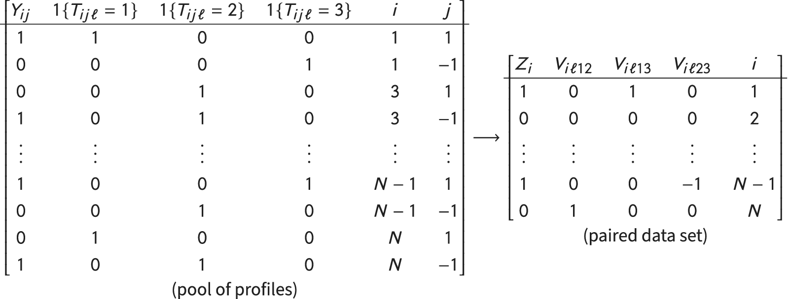
Figure 1 Pool of profiles and paired data set.

6.1 Estimation

In this framework, ACPs can be consistently estimated as

(10) $$ \begin{align} \hat{\hat{\pi}}_{\ell}(t_{\ell};w_{t_{\ell}})&=\sum_{\substack{t_{\ell}'\in\mathcal{T}_{\ell}\\t_{\ell}'\not=t_{\ell}}}w_{t_{\ell}}(t_{\ell}')\hat{\delta}_{t_{\ell}t_{\ell}'}, \end{align} $$

where $\hat {\delta }_{t_{\ell }t_{\ell }'}$ is the estimated average deviation of the selection probability of a $t_{\ell }$ -profile compared to a $t_{\ell }'$ -profile from the situation of indifference (where the selection probability is 0.5, that is). Noting that $\hat {\delta }_{t_{\ell }t_{\ell }'}=-\hat {\delta }_{t_{\ell }'t_{\ell }}$ , the coefficients $(\hat {\delta }_{\ell t_{\ell }t_{\ell }'})_{(t_{\ell },t_{\ell }')\in \mathcal {T}_{\ell }^2}$ can be obtained from a linear regression of $Z_i$ on a constant and the series of trichotomous variables $(V_{i\ell t_{\ell }t_{\ell }'})_{(t_{\ell },t_{\ell }')\in \mathcal {T}_{\ell }^2}$ :

(11) $$ \begin{align} Z_i=\alpha+\sum_{(t_{\ell},t_{\ell}')\in{\mathcal{T}}_{\ell}^2}\delta_{t_{\ell}t_{\ell}'}V_{i\ell t_{\ell}t_{\ell}'}+\Theta{\mathbf{V}}_{i[-\ell]}+\varepsilon_i, \end{align} $$

where $\mathbf {V}_{i[-\ell ]}\equiv \left (V_{i\ell ^{\prime } t_{\ell ^{\prime }}t_{\ell ^{\prime }}^{\prime }}\right )_{\substack {(t_{\ell ^{\prime }},t_{\ell ^{\prime }}^{\prime })\in \mathcal {T}_{\ell ^{\prime }}^2\\ \ell ^{\prime }\in \{1,\dots ,L\}\\ \ell ^{\prime }\not =\ell }}$ , for any i, and the inclusion of $\Theta \mathbf {V}_{i[-\ell ]}$ is optional for identification purposes. An interesting feature of this method is that it could also be used to estimate directly the entire vector of average preferences P, as $\hat {p}_{t_{\ell },t_{\ell }^{\prime }}=\hat {\delta }_{t_{\ell }t_{\ell }^{\prime }}$ (see the Supplementary Information D for an illustration).

When some attributes are conditionally independently randomized, an analogous method can be applied and CACPs can be estimated as

(12) $$ \begin{align} \hat{\hat{\pi}}_{\ell}(t_{\ell};w_{t_{\ell}}|T_{ij\ell'},T_{i[-j]\ell'})&=\sum_{\substack{t_{\ell}'\in\mathcal{T}_{\ell}\\t_{\ell}'\not=t_{\ell}}}w_{t_{\ell}}(t_{\ell}')\hat{\delta}_{t_{\ell}t_{\ell}'}(T_{ij\ell'},T_{i[-j]\ell'}), \end{align} $$

where the coefficients $\left (\hat {\delta }_{t_{\ell }t_{\ell }'}(T_{ij\ell '},T_{i[-j]\ell '})\right )_{\substack {t_{\ell }'\in \mathcal {T}_{\ell }\\t_{\ell }'\not =t_{\ell }}}$ could be obtained by fitting model (11) restricted to the pairs of profiles that meet the condition on $(T_{ij\ell '},T_{i[-j]\ell '})$ . The ACP for continuous attributes is simply obtained as the coefficient of the difference between attribute $\ell $ in both profiles in the regression of $Z_i$ on this difference and a constant. Finally, the identification assumption tests proposed by Hainmueller, Hopkins, and Yamamoto (Reference Hainmueller, Hopkins and Yamamoto2014) in the AMCE framework can be straightforwardly extended to the ACP framework.

7 Empirical Illustration

To illustrate the use and interpretation of ACPs, I calculate the ACPs for job experience, job plans, and occupations in Hainmueller and Hopkins’s (Reference Hainmueller and Hopkins2015; Hainmueller, Hopkins, and Yamamoto Reference Hainmueller, Hopkins and Yamamoto2013) immigrant experiment (Figure 2), using the R function available online (Ganter Reference Ganter2021). The occupation attribute is not fully independently randomized, but only conditional on education; financial analysts, research scientists, doctors, and computer programmers must also be assigned at least 2 years of college. In this case, I report ACPs conditional on a college education (unrestricted levels; orange diamonds) as well as ACPs conditional “comparable pairs” (blue squares).

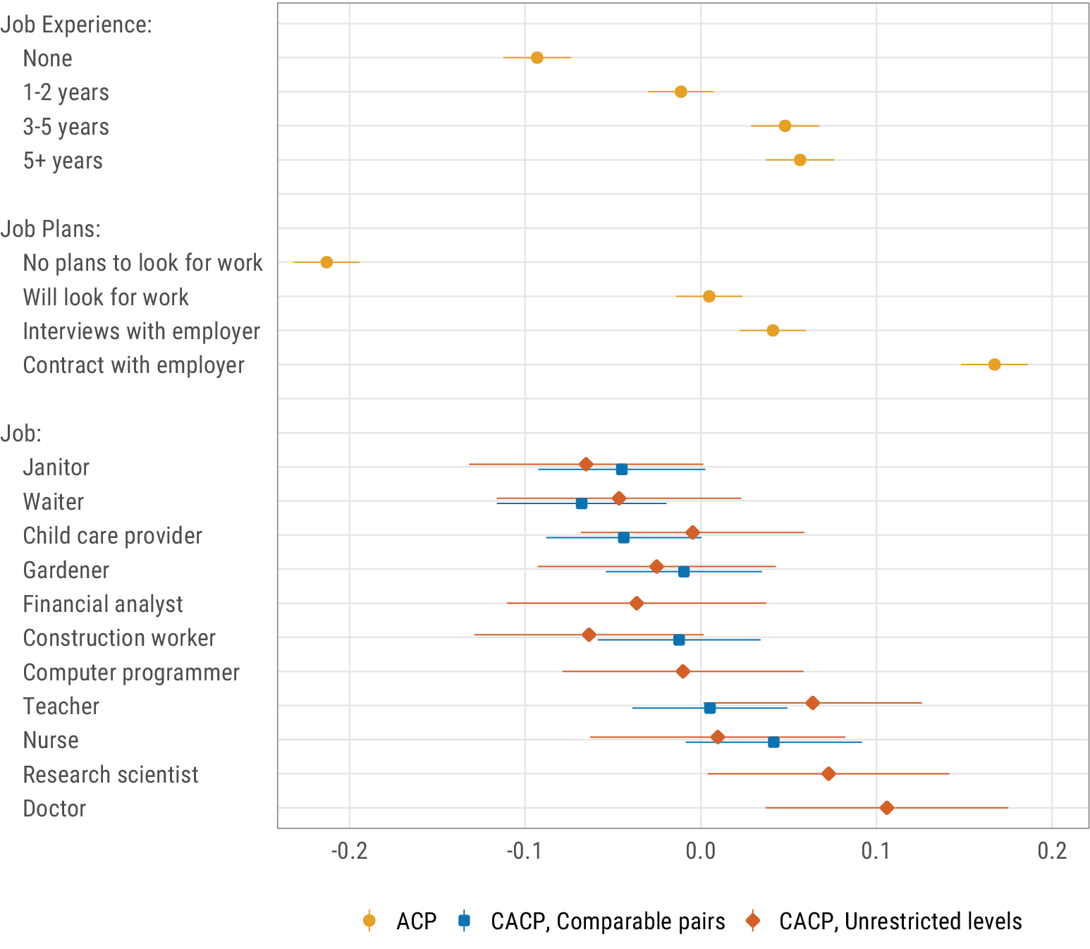
Figure 2 Preferences associated with immigrants’ job experience, job plans, and occupation measured by average component preferences (ACPs). Bars represent 95% confidence intervals with clustering at the respondent level. Partial replication of Hainmueller and Hopkins’s (Reference Hainmueller and Hopkins2015) immigrant experiment.

ACPs’ absolute values can be interpreted if we want to take each ACP as a standalone quantity. For example, the ACP for immigrants with no plans to look for work once in the United States is $-21.3$ ; when compared to an immigrant who will look for work or already has a contact with an employer, immigrants with no plans to look for work have a 28.7% ( $0.5-0.213$ ) chance to be selected for a visa. On the other hand, immigrants who already have a contract with an employer have a 66.7% ( $0.5+0.167$ ) chance to be selected for a visa when they are compared to an immigrant who does not have a contract.

Because preferences are relative, a more holistic approach to ACPs generally makes more sense than interpreting each ACP separately. For each attribute, the pattern of ACPs reflects the pattern of (average) preferences both in directionality and intensity. For example, respondents strongly prefer immigrants who already have a contract with an employer, and they have a strong reluctance to grant a visa to those who do not even plan to look for work once in the United States. Immigrants who do not have a contract yet but have plans to find a job in the United States occupy an intermediate position between both types, though they are closer to the former type. To interpret preference intensity, it may be helpful to use other attributes as benchmarks—which is possible because ACPs are comparable across attributes. As an example, having a contract rather than just planning on looking for work once in the United States has a roughly equivalent effect on respondents’ preferences as having more than 5 years of job experience rather than no experience at all.

The interpretation is slightly more complicated for conditionally independently randomized attributes because the CACPs are not all conditional on the same restriction. For the occupation attribute, CACPs represented by orange diamonds are conditional on a level of education at least equivalent to a 2-year college degree, whereas blue diamond CACPs are calculated for all “comparable pairs,” as I defined them earlier on. There might be differences between them. For example, while teachers are clearly preferred over construction workers among immigrants with a college degree, the difference is thin (and not statistically significant) when one includes immigrants with a lower level of education. There are two approaches here: If we want to examine preferences for occupations specifically—disentangled from preferences for education, that is—we need to compare ACPs of the same type (same color) only. On the contrary, if we are ready to take each occupation as a package that includes a specific distribution of education (so that doctors can be preferred because they have a higher level of education, and not only because of the job itself), cross-condition comparisons can be made.

Overall, these findings are consistent with the ones obtained with AMCEs; this is reassuring, but it should not be taken as a general rule. As a counter-example, I reanalyze the data from Mummolo and Nall’s (Reference Mummolo and Nall2017; Nall and Mummolo Reference Nall and Mummolo2016) experiment, in which the authors asked respondents to choose between two communities characterized by their housing cost, school quality, racial composition, and type of area, among other components. The authors seek to examine the relationship between people’s preferences (measured by the conjoint experiment, among other things) and people’s actual moving behavior; their conjoint analysis is thus clearly implemented to measure patterns of preferences. Here, I focus on school quality and on the type of place, and I do not distinguish between subgroups of respondents. Figure 3 reports AMCEs and ACPs for both attributes.

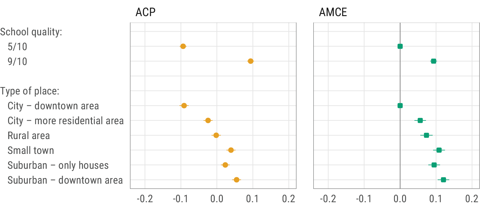
Figure 3 Preferences associated with communities’ type and school quality measured by average component preferences (ACPs) and average marginal component effects (AMCEs). Bars represent 95% confidence intervals with clustering at the respondent level. Partial replication of Mummolo and Nall’s (Reference Mummolo and Nall2017) community experiment.

Considering each attribute separately, both estimands tell a similar story: respondent prefer high school quality communities, and small towns or suburban areas over cities and, to a lesser extent, over rural areas. Yet, relying on AMCEs, one may want to conclude that the intensity of the type of place preference is similar to the intensity of the school quality preference, that is, both attributes are roughly similarly important for respondents. If anything, the former is even slightly more determinant than the latter, as the AMCE for suburban/downtown area is significantly bigger than the AMCE for a 9/10 school quality. ACPs point to a different conclusion, however; the range of school quality ACPs is substantially wider than the range of type of place ACPs, which suggests that school quality matters significantly more—not less—for respondents than the type of place. When exploring preferences, the ACP is the appropriate quantity of interest, so that the predominance of school quality over the type of place is the correct conclusion. Here, AMCEs under-estimate the importance of school quality. Specifically, they are misleading because there are more profiles tied on the school quality attribute (about 50%) than on the type of place attribute (about 17%). Mummolo and Nall’s (Reference Mummolo and Nall2017) argument goes beyond these two attributes and their main conclusions still hold, fortunately; what this example illustrates, however, is that the AMCE is not a reliable quantity for answering preference-related questions.