Introduction

Almost all electric power in Norway is produced in hydro-electric power plants, in general utilizing water stored in reservoirs at high altitudes or, to a smaller extent, utilizing river water with a relatively small head. Most of the rivers suitable for such low-head power production have been developed and the major remaining potential water power in Norway is therefore connected to high-head projects in mountainous areas. In general, these are situated in south-west and north Norway. Until recently all high-head power plants were located in almost glacier-free areas, but due to increased demand for water power it has been necessary to approach heavily glacierized basins for future developments. In general, these are three glacierized areas now considered for water power development:

the ice cap Folgefonni (south-east of Bergen),

the Jostedalsbre area (north of the Sognefjord),

the Svartisen area (in northern Norway close to the Arctic Circle).

A power station has already been installed at Mauranger, west of Folgefonni, and melt water from the western part of the ice cap contributes considerably to the high-altitude reservoirs constructed for this power station. Not less than 62 km² (or 38%) of the total catchment area (162 km²) is glacier-covered, so the glacier mass balance has a great influence on the annual inflow into the reservoirs. However, due to the short period this power station has been operating (only a few months) no experience has yet been gained concerning the impact of glacier variations on power production. It is, however, quite obvious that there will be a considerable variation in the amount of water available for power production between years of positive and years of negative mass balance.

This variation is expected to be somewhat diminished by the fact that years of positive glacier mass balance are often combined with “wet summers”, i.e. the liquid precipitation shows, in general, above-normal figures in years of glacier growth. Further, in most of these years the winter precipitation has also been heavy (in fact this is one of the reasons for a positive mass balance), and this snow adds considerably to the run-off from non-glacierized parts of the basin. Similarly, years of negative mass balance are mostly associated with less snow accumulation and, not least, with hot and dry summers.

The effect of glacier growth on river discharge in any given year would, theoretically, equal the total net balance, but the above-mentioned weather conditions will in most cases work in the opposite direction, and the impact on the annual inflow to the reservoirs due to glacier growth or shrinkage can be expected to be somewhat smaller than the total net balance.

An important glacierized area that will be developed in the future is the northern part of the ice cap Jostedalsbreen where a “roof-gutter system” will collect water at a relatively high altitude and store it in an artificial reservoir at an altitude of c. 1 000 m a.s.l. The production of electric energy will take place at a power plant close to sea-level, but some of the energy generated in summer time (during peak flood conditions) will be used to pump water up into the main reservoir (Fig. 1). This pumping is necessary because the peak power demand occurs during winter time, i.e. when the natural run-off from glacierized basins is at a minimum. Experience has shown that many glacier streams discharge about 80% of the annual run-off during only three months in the summer. A large water-storage capacity is therefore vital for a hydro-electric power-generating system utilizing glacier melt water. Substantial variations in expected water inflow, i.e. deviations from “normal” conditions, can be caused by glacier influence on river hydrology in glacierized basins and cause problems for storage management. A good knowledge of annual glacier variations, i.e. the net mass balance, is therefore important for an economically meaningful operation of many hydro-power systems in Norway.

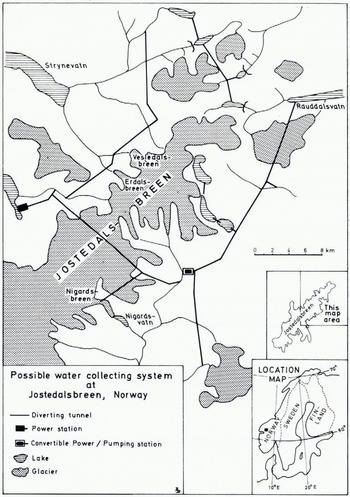
Fig. 1. It is proposed to utilize melt water from the north-eastern part of the ice-cap Jostedalsbreen and adjacent glaciers to produce hydro-electric energy in a power station at the lake Loenvatn (middle left). A system of tunnels collects water from numerous rivers in the area and some of the natural lakes will he dammed to form storage basins for power production in the winter.

Mass-Balance investigations

For planning purposes it is necessary for water-power engineers to obtain basic data on the expected run-off from glacierized basins. Therefore, mass-balance investigations were started on one outlet glacier from the ice cap Jostedalsbreen in 1962 (ØReference Østrem and Karléenstrem and Karlén, [1963]), and during the following years a selection of other glaciers were incorporated in the study program (ØReference Østrem and Liestølstrem, 1964; Østrem and LiestØl, 1964). Results from these mass-balance measurements have been used in various hydrological calculations. For example, several new river discharge gauging stations had been installed in the early 1960’s, mainly in basins considered for water-power development. However, annual discharge data from many such stations could not be used directly because glacier behaviour caused “errors” in the data material. The annual run-off proved to be much larger in years of glacier shrinkage and, correspondingly, too small during years of glacier growth. Therefore, one must apply a “correction” to the actually observed amount of water, by subtracting or adding a volume corresponding to glacier shrinkage or glacier growth for any given year. In this way a “normal” annual discharge can be calculated, i.e. the theoretical discharge that would appear if the glaciers were in a steady state. This involves detailed mass-balance studies on several glaciers, carefully selected to give representative data for the calculations.

Mass-balance investigations involve extensive field work and are expensive, and it is therefore important to try to find methods or means to reduce the overall costs for this kind of investigation. At present, Norges Vassdrags- og Elektrisitetsvesen conducts a program of continuous mass balance studies at some eight glaciers in Norway, and the mean cost for labour, transportation, etc., is of the order of $3 000-$ 10 000 per year per glacier under study.

The transient snow line

The transient snow line is defined as the lower border of last winter’s snow. On most glaciers it will be clearly visible as the border between a white blanket of last winter’s snow and the less white glacier ice or firn. It can be easily distinguished on air photographs (see Fig. 2) and its height can be determined from good topographic maps. The results from a study of the height of the transient snow line in western Canada is reported by ØReference Østremstrem (1973)-This study was based upon a great number of vertical air photographs taken simultaneously of a large number of glaciers in western Canada. The result indicated that the height of the transient snow line reached approximately similar altitudes for most glaciers within a certain area. It was also shown that the transient snow line (as of a given day) tends to reach higher altitudes in regions of increased continentality.

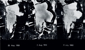
Fig. 2. The transient snow line can be seen an air photographs as the lower border of last winter’s snow. In years of heavy snow accumulation or little summer melt (or both) it does not climb very high up on the glacier (middle picture). In a year with more normal conditions it may reach a position close In the equilibrium line of the glacier at the end of the summer season (left-hand picture). During exceptionally hot summers it might reach the very highest parts of the glacier (right-hand picture). The pictures show the glacier Stuor Räitavagge in Sweden, approx. scale 1: 50 000.

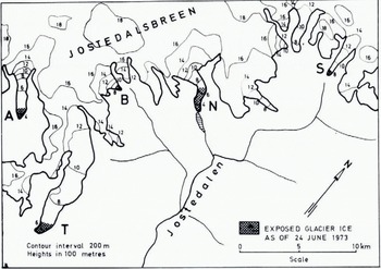
Fig. 3. From the ERTS image. No. 1336-10260 it was possible to determine areas of exposed ice on five outlet glaciers. The transient snow line appeared this year at an unusually low altitude due to heavy snowfalls lute in the spring.

Such studies cannot be repeated frequently for obvious reasons—it is unrealistic to request that extensive glacierized areas be re-photographed at intervals during one season or at the end of each summer. Therefore, it was hoped that data from the ERTS satellite would have a resolution sufficiently good to identify the transient snow line on glaciers. An 18 d imagery repetition would make possible a determination of the highest position of the transient snow line towards the end of the ablation season, and such information is most valuable, because it can be used for mass-balance studies, as we shall see below.

Results from erts-I

On the sixth day after launch, the ERTS satellite imaged the northernmost glacier in Scandinavia, the ice-cap Seilandsjøkulen, and the transient snow line was clearly shown, particularly in MSS-7. During the rest of the summer 1972 the weather conditions unfortunately prevented further useful imagery of glacierized areas suitable for studies of the transient snow line, but it was quite clear that it could be identified on ERTS images.

The next useful ERTS image was obtained on 24 June 1973. From this image (No. 1336-10260) it was possible to determine the height of the transient snow line on five outlet glaciers from the ice cap Jostedalsbreen (sec Fig. 3). It was, however, not possible to follow the increase in snow-line heights throughout that summer because no more good ERTS images were obtained during the melt season. This was, of course, due to technical limitations on board the spacecraft, combined with weather conditions.

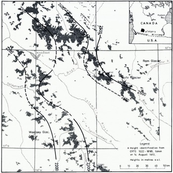
Fig. 4. The height of the transient snow line was determined on 36 individual glaciers and contours were drawn for a theoretical surface intersecting the landscape at a height corresponding to the transient snow line position as of 14 August 1972.

Due to lack of good images from Scandinavia the author continued similar work on images taken over the Canadian Rocky Mountains. On two different occasions it was possible to determine the height of the transient snow line on a relatively large number of glaciers, viz. on 14 August 1972 and on 8-9 August 1973. The results are shown in Figures 4, 5, 6 and 7.

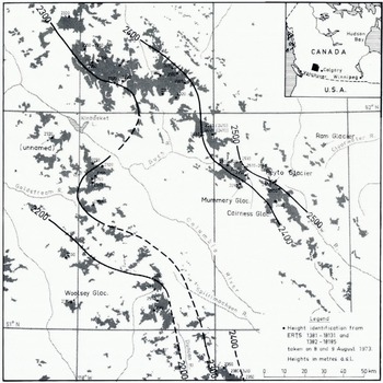
Fig. 5. From two ERTS images obtained on two consecutive days a similar determination was made as shown in Figure 4, this time on 40 glaciers. When contour lines were drawn a similar pattern was found as for the situation obtained in 1972. Note that some glaciers always show a snow-line height deviating from the “normal”. For example, in both years the Mummery Glacier showed an altitude 100 m lower than could be expected in that area, whereas an unnamed glacier south west of Kinbasket Lake indicated both years too high a figure. Apart from stich single deviations, the transient snow line will be located at similar altitudes within the same mountain massif (as of a given day).

The relation between transient snow line and mass balance

There exists an obvious connection between the height of the transient snow line at the end of the summer and the glacier’s net mass balance: for example, during years of strongly negative mass balance the transient snow line will reach its highest positions, and vice versa. Further, on most temperate glaciers, the transient snow line will, in any given year, climb to a height which is almost identical with the height of the equilibrium line for that year. Only in cases where the glacier surface happens to be fairly flat it is possible that a zone of superimposed ice might be seen between areas of last winter’s snow and areas of completely uncovered glacier ice (compare Fig. 2, left-hand part). If such a picture is obtained at the end of the melt season, the equilibrium line will be situated at the lower edge of the superimposed ice zone, because superimposed ice is a part of the last winter’s accumulation on the glacier surface. Apart from this small difference in position caused by the presence of some superimposed ice, it is relevant in this connection to use the height of the transient snow line (as seen on air photographs or on satellite images) to indicate the height of the equilibrium line for a given glacier.

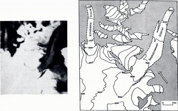
Fig. 6. Fig. G. A part of ERTS image. No. 1332-18185 taken on 9 August 1973 over the Canadian Rocky Mountains showing the Saskatchewan and Athabasca Glaciers (left). The map is redrafted from the Canadian Topographic Map System 83 C 3-Columbia Icefield (right). Transient snow lines can he seen on the image, and their altitude determined from the contour map. Compare Figures 4 and 5, where results for larger regions are shown. Contour heights are shown in feet on this map, but were converted to metres when results were plotted on Figures 4 and 5

Results from current mass-balance investigations in Canada and in Scandinavia (see, for example, Reference SchyttSchytt, 1966, p. 44-46) indicate that there is a good correlation between the specific net mass balance and the height of the equilibrium line at the end of the melt season (cf. Figs 8 and 9). Consequently, if the height of the transient snow line could be determined by satellite imagery, this would be a valuable tool in mass-balance investigations.

Before the satellite data can be used for this kind of glaciological work, it is necessary that detailed mass-balance studies have already been performed throughout a series of years, so that the above-mentioned correlation has been established. Ideally both years of negative and of positive net mass balance should be represented in the observation series, so that a correlation diagram can be constructed comprising the widest possible range of net mass-balance conditions (compare Fig. 9). For glaciers where mass-balance studies have been performed during a long series of years, it might happen that improved field techniques, etc. make it necessary to select the most reliable results and discard other, in general older, results (compare Reference SchyttSchytt, 1967, p. 329) before the diagram is constructed. Provided a good satellite imagery is obtained at the end of a summer season, the height of the transient snow line can be easily determined from a topographic map and, finally, the specific net mass balance is found from the correlation diagram (of the type shown in Fig. 9).

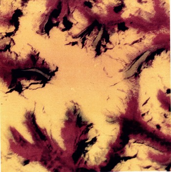
Fig. 7. Part of ERTS image No. 1741-18045 taken on 3 August 1974, showing the Columbia Icefield and its outlet glacier..

This colour composite picture was generated in an additive projector from positive transparencies supplied by the Canadian Centre for Remote Sensing. The following colours were used: MSS 5-green, MSS 7-red. This colour combination gave, in this case, the best contrast for determination of the transient snowline-with yellow snow fields and a blue-green colour on exposed glacier ice. Vegetation shows up in red, whereas black indicates areas of dark shadow or clear-water lakes Silty water will be shown in a dark greenish colour. Suck lakes would be more emphasized if MSS 4 were also included m the production of the, colour composite picture, but this was not done because the main objective was to identify transient snow lines.

For scale and orientation, compare with the map in Figure 6, right-hand part. The outlet glacier to the left is Columbia Glacier. On the original, silty lakes can be seen in front of the Columbia Glacier and the Athabasca Glacier. (Colour selection by S. Smith-Meyer, Photograph by H. P. østrem.)

Fig. 8. There is a definite relation between the height of the equilibrium line at the end of the ablation season and the specific net mass balance. This diagram is based upon annual mass-balance investigations performed by the Canadian Department of Energy, Mines and Resources and Department of the Environment since 1965 (personal communication from A. Stanley).

Obviously one is thus obtaining only the specific net mass balance for a given glacier—no separate information will be available regarding the winter balance or the summer balance. However, for engineering purposes a single figure for the specific net balance is sufficient; this is used in the hydrological calculations to obtain a “normal” run-off figure for glacierized basins.

For most glaciological studies on the other hand, and particularly for detailed studies of winter accumulation and summer melt or relations between weather conditions and mass balance, results produced by this method cannot compete at all with data obtained by conventional methods, i.e. mainly field work on the glacier proper.

Use of digital data

The method mentioned above is based upon analogue data from ERTS—i.e. the data are in general given as four black-and-white images, one for each of the spectral bands. On such images, provided by NASA as transparancies or photographic prints, it is possible to distinguish between a maximum of 15 grey-scale levels. This number of grey-scale levels, and the contrast in the products delivered, is sufficient to allow the interpreter to distinguish between areas of snow or ice and areas of snow-free ground (in MSS-4) and the images are also useful to distinguish between snow and ice (in MSS-7). However, to investigate whether a more detailed analysis could be done directly from digital data (computer-compatible magnetic tape) an experiment was carried out with a selected ERTS scene. The glacier Seilandsjøkulen and adjacent ground were selected for the study, and this section was taken from a magnetic tape provided by NASA (ERTS No. 1006-09481).

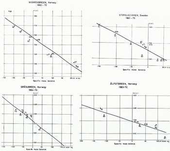
Fig. 9. Correlation diagrams for some Scandinavaian glaciers were construct to demonstrate the relation between the height of the equilibrium live and specific mass balance. In some cases a single year’s observations are missing, because it happened that the transient snow line was located below or above the glacier (i.e. the glacier was completely snow-covered or snow-free at the end of the summer), and thus its height could not be defined.

A line-printer map of the glacier was produced from the original MSS-7 data, (see Fig. 10) and a further analysis showed that the reflectance from last winter’s snow, as seen from ERTS on 29 July 1972, was represented by the grey scale levels 41-48. There is provided a 63-level scale in the digital data, so an even higher brightness can be recorded, although the snow was shown as completely white areas on the photographic images. Further, glacier ice was represented by grey scale levels 13-20 whereas adjacent bedrock had only a slightly lower brightness represented by levels 7—12.

Fig. 10. A “map” produced by a computer line printer from ERTS-I digital data (MSS-7). The white areas represent last winter’s snow whereas grey areas represent exposed glacier ice on the ice cap Seilandsjøkulen in northern Norway. Darker areas indicate bedrock or water. Each letter or sign {with a surrounding rim) indicates one “pixel” which covers 56m X 79 m on the ground. Approximate scale 1: 50 000. The computer program used for the construction of this map was written by I. Akersten.

In band MSS-4, however, last winter’s snow gave a much higher reflectance, represented by a grey-scale level ranging from 55-62, and glacier ice gave levels 39-44 on the 63-level scale. Thus, the difference between snow and ice was less pronounced in MSS-4 than in MSS-7. On the analogue MSS-4 material (transparencies or prints) it was not possible to see any difference between snow and ice at all. (Note: the grey-scale levels quoted above are only correct for a given latitude and a given date, because the effect of solar angle on brightness needs to be considered before one can extrapolate or generalize the results to different times or different localities.)

By this digital method it may be possible to automate determination of the transient snow line, and areas covered by last winter’s snow (or the entire glacier surface) may be measured automatically, but so far only relatively simple experiments have been made and more research is necessary along these lines.

Conclusion

Images or digital data from the ERTS-I satellite have been used to determine the position of the transient snow line on glaciers and its height has been found by comparison with topographic maps. This method is in general similar to a method utilized in the past when conventional air photographs were used. There seems to be a (linear) relationship between the height of the transient snow line at the end of the summer season and the specific net mass balance. This makes possible a determination of the net mass balance for a glacier from ERTS data if they are obtained at the end of the ablation season, provided detailed mass-balance studies throughout a series of years have been made at the glacier in question, so that the said relationship is known. Digital data may in the future be better to use for the determination of the transient snow line on glaciers, but a standard program for such work has not yet been developed.