


1. Introduction
Hot subdwarf stars are located at the extreme blue end of the horizontal branch in the Hertzsprung–Russell diagram (Heber Reference Heber2016). They divide into different types, depending on spectroscopic parameters (sdB, sdOB, sdO, He-sdB, and He-sdO – see Baran et al. Reference Baran2023, for details) and observations show that sdB stars are the most common. This work is a continuation of our efforts to detect new hot subdwarf pulsators, understand their internal structure, and connect it to Galactic populations. Hot subdwarfs have a surface gravity
 $\log{(g/\mathrm{cm}\,\mathrm{s}^{-2})}$
of 5.0–5.8, which indicates that they are compact. In fact, their radii are in a range of 0.15–0.35 R
$\log{(g/\mathrm{cm}\,\mathrm{s}^{-2})}$
of 5.0–5.8, which indicates that they are compact. In fact, their radii are in a range of 0.15–0.35 R
 $_{\odot}$
and their total masses are around 0.5 M
$_{\odot}$
and their total masses are around 0.5 M
 $_{\odot}$
(Heber Reference Heber2016). According to Figure C4 presented by Ostrowski et al. (Reference Ostrowski, Baran, Sanjayan and Sahoo2021) the masses can be as low as almost 0.3 M
$_{\odot}$
(Heber Reference Heber2016). According to Figure C4 presented by Ostrowski et al. (Reference Ostrowski, Baran, Sanjayan and Sahoo2021) the masses can be as low as almost 0.3 M
 $_{\odot}$
, and they can go beyond 0.5 M
$_{\odot}$
, and they can go beyond 0.5 M
 $_{\odot}$
in case of a few solar mass progenitors. The interiors of hot subdwarfs consist of a convective helium core in which helium fusion takes place, surrounded by a helium shell. The outermost layer is a very thin (in mass) hydrogen envelope of less than 10
$_{\odot}$
in case of a few solar mass progenitors. The interiors of hot subdwarfs consist of a convective helium core in which helium fusion takes place, surrounded by a helium shell. The outermost layer is a very thin (in mass) hydrogen envelope of less than 10
 $^{-2}\,\textit{M}_{\odot}$
. Such an envelope is a unique mark of hot subdwarfs and is a consequence of some mass loss mechanisms during red-giant branch evolution. The mass loss can be explained by stellar binarity (Han et al. Reference Han, Podsiadlowski, Maxted, Marsh and Ivanova2002, Reference Han, Podsiadlowski, Maxted and Marsh2003), substellar companions (Charpinet et al. Reference Charpinet, Giammichele, Zong, Grootel, Brassard and Fontaine2018), or a strong stellar wind (Fontaine et al. Reference Fontaine, Brassard, Charpinet, Green, Randall and Van Grootel2012). The effective temperature of these stars ranges from 20 000 to 40 000 K. The lack of a massive hydrogen envelope makes hot subdwarfs skip the asymptotic giant branch and evolve directly towards white dwarf cooling tracks. Hot subdwarfs were found in Galactic field populations (Altmann et al. Reference Altmann, Edelmann and de Boer2004; Martin et al. Reference Martin and Jeffery2016), old open clusters (Kaluzny and Ruciński Reference Kaluzny and Rucinński1993), and globular clusters (Moehler Reference Moehler2001; Moni Bidin et al. Reference Moni Bidin, Catelan, Villanova, Piotto, Altmann, Momany, Moehler, Heber, Jeffery and Napiwotzki2008).
$^{-2}\,\textit{M}_{\odot}$
. Such an envelope is a unique mark of hot subdwarfs and is a consequence of some mass loss mechanisms during red-giant branch evolution. The mass loss can be explained by stellar binarity (Han et al. Reference Han, Podsiadlowski, Maxted, Marsh and Ivanova2002, Reference Han, Podsiadlowski, Maxted and Marsh2003), substellar companions (Charpinet et al. Reference Charpinet, Giammichele, Zong, Grootel, Brassard and Fontaine2018), or a strong stellar wind (Fontaine et al. Reference Fontaine, Brassard, Charpinet, Green, Randall and Van Grootel2012). The effective temperature of these stars ranges from 20 000 to 40 000 K. The lack of a massive hydrogen envelope makes hot subdwarfs skip the asymptotic giant branch and evolve directly towards white dwarf cooling tracks. Hot subdwarfs were found in Galactic field populations (Altmann et al. Reference Altmann, Edelmann and de Boer2004; Martin et al. Reference Martin and Jeffery2016), old open clusters (Kaluzny and Ruciński Reference Kaluzny and Rucinński1993), and globular clusters (Moehler Reference Moehler2001; Moni Bidin et al. Reference Moni Bidin, Catelan, Villanova, Piotto, Altmann, Momany, Moehler, Heber, Jeffery and Napiwotzki2008).
A goal of the kinematic study of stars is to derive their galactic population membership and relationships between populations and specific stellar parameters. Such a study requires large samples of stars for which galactic orbits can be derived. Most of the studies of hot subdwarfs delivered only population membership assignments with no report of a relation between pulsation content and Galactic populations. Colin et al. (Reference Colin1994) determined space velocities and orbits for seven stars and concluded on their Galactic populations. Altmann et al. (Reference Altmann, Edelmann and de Boer2004) performed a kinematic survey of 114 hot subdwarfs. They used space velocities, eccentricities, and angular momenta of their galactic orbits and found that a vast majority of the stars show a kinematic behaviour that is similar to that of thick disc stars. Recently, Luo et al. (Reference Luo, Németh, Wang, Wang and Han2021) performed an extensive kinematics study of 1587 subdwarfs by using precise and uniform Gaia DR2 astrometry and LAMOST DR7 spectroscopy data. The authors derived Galactic population memberships of these stars and tried to find a correlation between the helium content and the membership but came with no conclusions because of a limited sample.
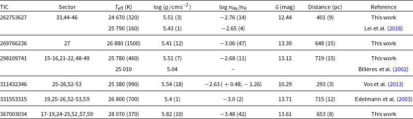
Table 1. Information for the six stars analysed in our work. The ‘Reference’ column refers to the spectroscopic parameters only.
A small subset (around 10%, Østensen et al. Reference Østensen2010; Reed et al. Reference Reed, Slayton, Baran and Telting2021) of hot subdwarfs shows pulsations in pressure (p) modes, gravity (g) modes, or both (hybrids). Stellar pulsations provide us with a pathway to understand their internal structures through asteroseismology (Charpinet et al. Reference Charpinet, Fontaine, Brassard, Chayer, Rogers, Iglesias and Dorman1997). In most cases, p-modes, with typical periods of minutes, provide information about the outer regions, whereas g-modes, with typical periods of hours, probe deeper regions (Heber Reference Heber2016).
The Transiting Exoplanet Survey Satellite (TESS; Ricker et al. Reference Ricker2014) is an all-sky survey whose prime mission is to detect exoplanets orbiting nearby bright stars using the transit method. Apart from its prime mission, it also provides time-series photometry of a large sample of stars, which can be used for other goals, including asteroseismology. We only included a selection of results of analyses of hot subdwarf pulsators derived with TESS. Charpinet et al. (Reference Charpinet2019) presented a detailed asteroseismic analysis of EC 21494–7018 (TIC 278659026), a pulsating sdB star with 20 gravity modes, which was monitored in the short cadence (SC) mode (2 min). Reed et al. (Reference Reed2020) reported analysis of CD – 28
 $^{\rm o}$
1974. They found the gravity-mode frequency range to be slightly different than the typical for these stars and concluded that the star must have a different internal structure. Sahoo et al. (Reference Sahoo2020a) presented a detailed mode identification and atmospheric analyses of three pulsating hot subdwarfs. Uzundag et al. (Reference Uzundag2021) presented photometric and spectroscopic analyses of five gravity-mode hot subdwarf pulsators observed in the SC, as well as ultra-short cadence (20 sec) modes. Silvotti et al. (Reference Silvotti, Németh, Telting and Baran2022) reported an analysis of a hot subdwarf pulsator, TYC 4544-2658-1, found to be a non-synchronised binary system with the shortest orbital and core rotation periods. The authors reported rotationally split modes, provided a mode identification, and matched observed pulsation periods with modelled ones. Sahoo et al. (Reference Sahoo, Baran, Sanjayan and Ostrowski2020b) and Baran et al. (Reference Baran, Sahoo, Sanjayan and Ostrowski2021) used TESS Full Frame Images to find new variable hot subdwarfs and performed mode identification for a few pulsators. Baran et al. (Reference Baran2023) presented a list of p-mode hot subdwarf pulsators observed by TESS. We report the results of our analysis of the TESS photometry of six hot subdwarf pulsators, that is, TIC 262753627, TIC 269766236, TIC 298109741, TIC 311432346, TIC 331553315, and TIC 367003034. We selected six stars with a moderate number of g-modes, which can be identified using asymptotic period spacing, followed by pulsation periods fitting. Prior to this work, only for five pulsating hot subdwarfs MESA and GYRE models (acronyms are explained in Section 4) were used to derive stellar parameters (Silvotti et al. Reference Silvotti, Németh, Telting and Baran2022; Baran & Sanjayan Reference Baran and Sanjayan2023).
$^{\rm o}$
1974. They found the gravity-mode frequency range to be slightly different than the typical for these stars and concluded that the star must have a different internal structure. Sahoo et al. (Reference Sahoo2020a) presented a detailed mode identification and atmospheric analyses of three pulsating hot subdwarfs. Uzundag et al. (Reference Uzundag2021) presented photometric and spectroscopic analyses of five gravity-mode hot subdwarf pulsators observed in the SC, as well as ultra-short cadence (20 sec) modes. Silvotti et al. (Reference Silvotti, Németh, Telting and Baran2022) reported an analysis of a hot subdwarf pulsator, TYC 4544-2658-1, found to be a non-synchronised binary system with the shortest orbital and core rotation periods. The authors reported rotationally split modes, provided a mode identification, and matched observed pulsation periods with modelled ones. Sahoo et al. (Reference Sahoo, Baran, Sanjayan and Ostrowski2020b) and Baran et al. (Reference Baran, Sahoo, Sanjayan and Ostrowski2021) used TESS Full Frame Images to find new variable hot subdwarfs and performed mode identification for a few pulsators. Baran et al. (Reference Baran2023) presented a list of p-mode hot subdwarf pulsators observed by TESS. We report the results of our analysis of the TESS photometry of six hot subdwarf pulsators, that is, TIC 262753627, TIC 269766236, TIC 298109741, TIC 311432346, TIC 331553315, and TIC 367003034. We selected six stars with a moderate number of g-modes, which can be identified using asymptotic period spacing, followed by pulsation periods fitting. Prior to this work, only for five pulsating hot subdwarfs MESA and GYRE models (acronyms are explained in Section 4) were used to derive stellar parameters (Silvotti et al. Reference Silvotti, Németh, Telting and Baran2022; Baran & Sanjayan Reference Baran and Sanjayan2023).
2. TESS photometry and ground-based spectroscopy
TESS provided data for all six targets in the SC mode and for TIC 298109741, TIC 311432346, TIC 331553315, and TIC 367003034 in the USC mode, which became available only with the onset of the extended mission. We downloaded the data from the Mikulski Archive for Space Telescopes (MAST) database. Only TIC 269766236 was observed during a single sector covering about 27 days. The remaining five stars were monitored over multiple sectors, ranging from four to eight for the longest data coverage. We combined datasets if they were collected during a single observing cycle and provided roughly the same solutions as compared to those derived from shorter chunks; with the exception of frequencies that are low amplitude and did not meet the threshold criterion, as a consequence of a higher noise level in amplitude spectra in shorter chunks of data. More details of each star are given in Table 1. We used PDCSAP_FLUX measures, which account for onboard systematics and a contribution from neighbouring stars. We detrended variations longer than one day and converted the fluxes to a parts per thousand (ppt) unit. We used Lightkurve (Lightkurve Collaboration et al. 2018) to process the data.
We collected atmospheric parameters of TIC 262753627, TIC 298109741, TIC 311432346, and TIC 331553315 from the literature and listed them in Table 1. In addition, we acquired an existing LAMOST spectrum of TIC 262753627, and we collected spectroscopic observations of TIC 269766236 with the 1.9 m telescope at the South African Astronomical Observatory (SAAO), of TIC 298109741 with the Dual Imaging Spectrograph at Apache Point Observatory, and of TIC 367003034 with the Hanle Faint Object Spectrograph Camera (HFOSC) of 2 m Himalayan Chandra Telescope (HCT) at the Indian Astronomical Observatory (IAO). Details of our spectroscopic observations are listed in Table 2.
Table 2. Details of spectroscopic observations of four stars observed using ground-based telescopes.
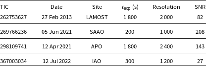
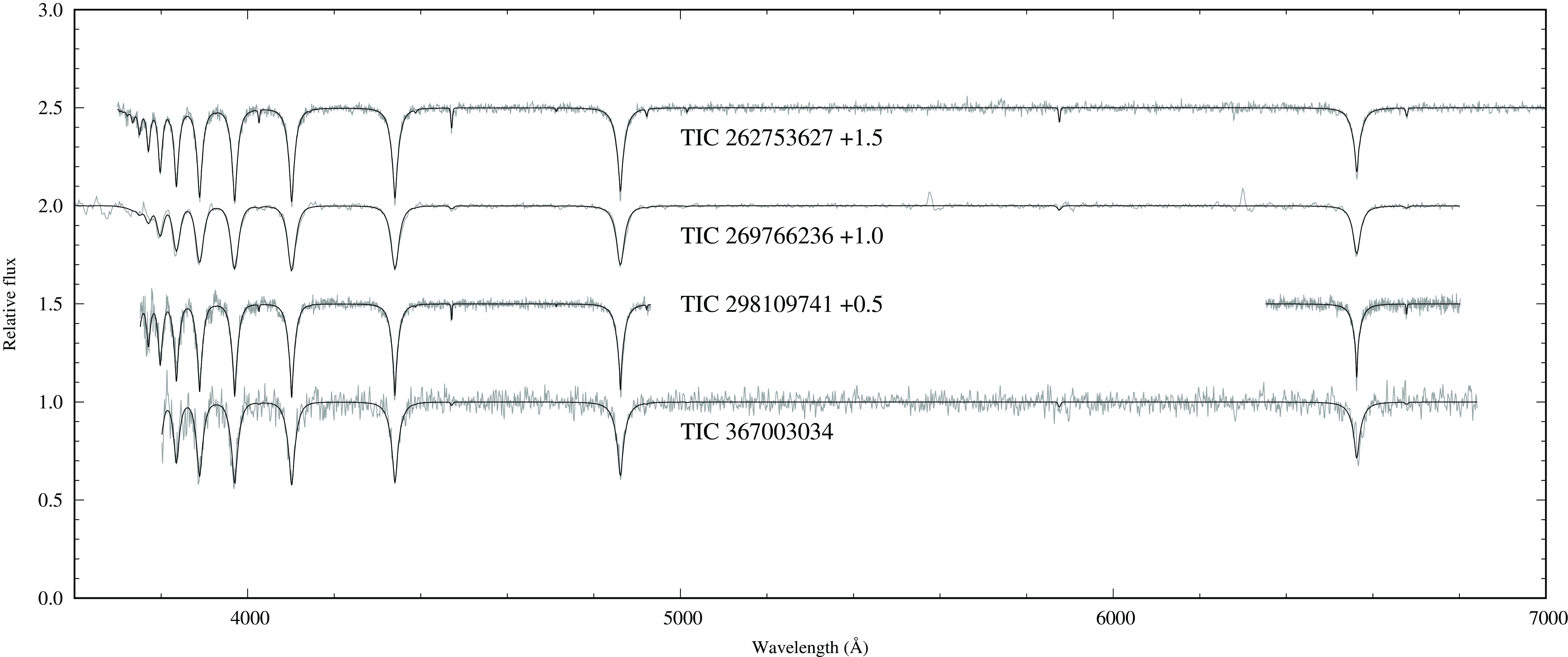
Figure 1. Best-fit Tlusty/XTgrid models to the various observations of the program stars: TIC 262753627 (LAMOST), TIC 269766236 (SAAO), TIC 298109741 (APO), and TIC 367003034 (HFOSC). In all cases, observations are in grey and the models are in black.
We analysed the spectra with the data-driven steepest-descent
 $\chi^2$
minimisation spectral analysis program XTgrid (Németh et al. Reference Németh, Kawka and Vennes2012) to determine effective temperature (
$\chi^2$
minimisation spectral analysis program XTgrid (Németh et al. Reference Németh, Kawka and Vennes2012) to determine effective temperature (
 $T_\mathrm{eff}$
), surface gravity (
$T_\mathrm{eff}$
), surface gravity (
 $\log\,g$
), and helium abundance (n
$\log\,g$
), and helium abundance (n
 $_{\mathrm{He}}$
/n
$_{\mathrm{He}}$
/n
 $_{\mathrm{H}}$
). The fitting procedure is an interface to calculate non-LTE (non-Local Thermodynamic Equilibrium) stellar atmosphere models and synthetic spectra with Tlusty/Synspec (Hubeny and Lanz Reference Hubeny and Lanz1995, Reference Hubeny and Lanz2017) and to fit them to observations. The theoretical models are matched to the observations with piecewise normalisation, and the model parameters are varied iteratively along the steepest gradient of the global
$_{\mathrm{H}}$
). The fitting procedure is an interface to calculate non-LTE (non-Local Thermodynamic Equilibrium) stellar atmosphere models and synthetic spectra with Tlusty/Synspec (Hubeny and Lanz Reference Hubeny and Lanz1995, Reference Hubeny and Lanz2017) and to fit them to observations. The theoretical models are matched to the observations with piecewise normalisation, and the model parameters are varied iteratively along the steepest gradient of the global
 $\chi^2$
until the fit converges to the best solution. The normalisation method reduces the effects of the uncalibrated continuum flux and the fit is based on the relative strengths and profiles of the spectral lines. The fitting procedure iterates the models until the relative changes of all model parameters and the
$\chi^2$
until the fit converges to the best solution. The normalisation method reduces the effects of the uncalibrated continuum flux and the fit is based on the relative strengths and profiles of the spectral lines. The fitting procedure iterates the models until the relative changes of all model parameters and the
 $\chi^2$
decrease below 0.1% over three consecutive iterations. Then, parameter errors are calculated by mapping the
$\chi^2$
decrease below 0.1% over three consecutive iterations. Then, parameter errors are calculated by mapping the
 $\chi^2$
variations around the best solution. For
$\chi^2$
variations around the best solution. For
 $T_{\mathrm{eff}}$
and
$T_{\mathrm{eff}}$
and
 $\log{g}$
, this includes the correlations in two dimensions, and for the He abundance it is done in one dimension. If a better solution is found during error calculations XTgrid returns to iterations with the local minimum as starting point. More details on the procedure can be found in Németh et al. (Reference Németh, Kawka and Vennes2012).
$\log{g}$
, this includes the correlations in two dimensions, and for the He abundance it is done in one dimension. If a better solution is found during error calculations XTgrid returns to iterations with the local minimum as starting point. More details on the procedure can be found in Németh et al. (Reference Németh, Kawka and Vennes2012).
Our models included H and He opacities in both the stellar structure calculations and the spectral synthesis. The final parameters are listed in Table 1, and the best-fit models are shown in Fig. 1. Parameter degeneracies are large in low-resolution spectroscopy, which are reflected by the large measured statistical errors. A significantly larger systematic error than degeneracies is introduced by calibration issues, and flexure, which affected the SAAO spectrum. The large parameter uncertainties for TIC 269766236 are due to the non-symmetric and non-Gaussian instrumental profile of grating #7 of the SpUpNIC spectrograph on the 1.9 m telescope at SAAO (Figure 21 in Crause et al. Reference Crause2019).
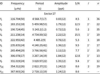
Table 3. Frequencies detected in amplitude spectra of TIC 262753627. An apostrophe sign denotes signals taken for analysis presented in Section 4.
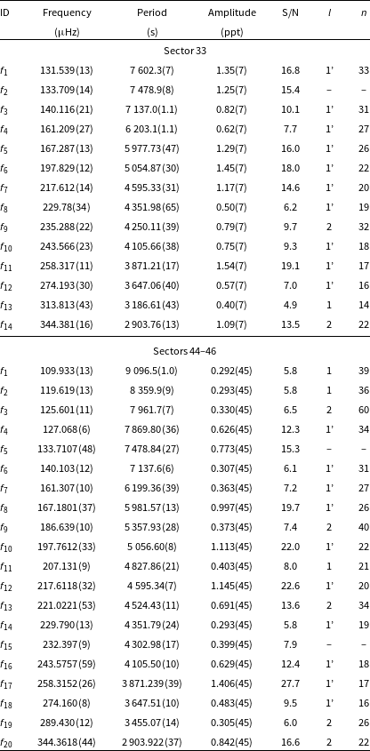
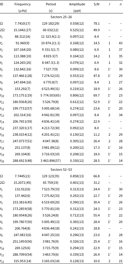
Table 4. Frequencies detected in an amplitude spectrum of TIC 269766236.
3. Fourier analysis and mode identification
We calculated amplitude spectra, and we applied a standard prewhitening process with Period04 (Lenz and Breger Reference Lenz and Breger2005). We fitted significant signal with
 $A_{{i}}\sin(2{\pi}\mathrm{f}_{\mathrm{i}}\mathrm{t}+{\phi_{\mathrm{i}}}$
) using a nonlinear least-square method. The symbols used have usual meaning, that is, A is amplitude, f is frequency,
$A_{{i}}\sin(2{\pi}\mathrm{f}_{\mathrm{i}}\mathrm{t}+{\phi_{\mathrm{i}}}$
) using a nonlinear least-square method. The symbols used have usual meaning, that is, A is amplitude, f is frequency,
 $\phi$
is phase, while ‘i’ iterates through the sinusoidal terms. We limited the detection threshold to be five times the median noise (N) level (Baran andKoen Reference Baran and Koen2021), which was calculated from residual amplitude spectra in the range of 1 000–4 000
$\phi$
is phase, while ‘i’ iterates through the sinusoidal terms. We limited the detection threshold to be five times the median noise (N) level (Baran andKoen Reference Baran and Koen2021), which was calculated from residual amplitude spectra in the range of 1 000–4 000
 $\mu$
Hz. The corresponding Nyquist frequency is 4 166
$\mu$
Hz. The corresponding Nyquist frequency is 4 166
 $\mu$
Hz. We detected no signal beyond 4 166
$\mu$
Hz. We detected no signal beyond 4 166
 $\mu$
Hz in the USC data, hence we limit our analyses only to the SC mode for all six targets. A few frequencies with amplitudes lower than the threshold, listed in Tables 3, 4, and 7, should be considered tentative. We discuss details of our prewhitening and mode identification for each target in the paragraphs below.
$\mu$
Hz in the USC data, hence we limit our analyses only to the SC mode for all six targets. A few frequencies with amplitudes lower than the threshold, listed in Tables 3, 4, and 7, should be considered tentative. We discuss details of our prewhitening and mode identification for each target in the paragraphs below.
Table 5. Frequencies detected in amplitude spectra of TIC 298109741.
We determined the mode degree using the asymptotic period spacing, widely applied and described in previous works (Østensen et al. Reference Østensen, Telting, Reed, Baran, Nemeth and Kiaeerad2014). In the asymptotic limit (
 $n \gg l$
), consecutive g-mode overtones, for a given degree, are evenly spaced in period. An average period spacing of dipole modes (l=1) ranges from 230 to 270 s (e.g. Reed et al. Reference Reed2020; Sahoo et al. Reference Sahoo2020a
). We started our modal degree assignment from the highest amplitude frequencies and assigned them dipole modes if a period spacing was a multiple of about 250 s. Next, other frequencies with lower amplitudes, but spaced as the highest amplitude counterparts, were also assigned with dipole modes. Our choice can be justified by the surface cancellation effect (Dziembowski Reference Dziembowski1977), which dilutes an amplitude as the mode degree increases by approximately (1/
$n \gg l$
), consecutive g-mode overtones, for a given degree, are evenly spaced in period. An average period spacing of dipole modes (l=1) ranges from 230 to 270 s (e.g. Reed et al. Reference Reed2020; Sahoo et al. Reference Sahoo2020a
). We started our modal degree assignment from the highest amplitude frequencies and assigned them dipole modes if a period spacing was a multiple of about 250 s. Next, other frequencies with lower amplitudes, but spaced as the highest amplitude counterparts, were also assigned with dipole modes. Our choice can be justified by the surface cancellation effect (Dziembowski Reference Dziembowski1977), which dilutes an amplitude as the mode degree increases by approximately (1/
 $\sqrt{l}$
). In our analyses, the majority of the detected frequencies are dipole modes, hence we only calculated the average period spacings for dipole modes. We used a linear regression to derive average period spacings and uncertainties of dipole modes. We calculated the average period spacings and their uncertainties for quadrupole modes from equation
$\sqrt{l}$
). In our analyses, the majority of the detected frequencies are dipole modes, hence we only calculated the average period spacings for dipole modes. We used a linear regression to derive average period spacings and uncertainties of dipole modes. We calculated the average period spacings and their uncertainties for quadrupole modes from equation
 $\Delta P_{l\,=\,2}\,=\,\Delta P_{l\,=\,1}/\sqrt{3}$
. Since we found no multiplets in any of our targets, the mode assignment based solely on the period spacing sequences may not always be correct.
$\Delta P_{l\,=\,2}\,=\,\Delta P_{l\,=\,1}/\sqrt{3}$
. Since we found no multiplets in any of our targets, the mode assignment based solely on the period spacing sequences may not always be correct.
Most frequencies were identified as dipole modes with just a handful of exceptions for each target. After determining the dipole modes, we tried to match the rest of the spacing with the quadrupole sequence. But we stress that due to very limited numbers of detected quadrupole modes, the trends in the échelle diagrams are more scattered and these solutions may not be unique. Periods not matching either dipole or quadrupole sequences were marked as unidentified. As described in Sahoo et al. (Reference Sahoo2020a) the radial order n is not absolute. Based on our mode assignment, we calculated échelle diagrams for dipole and quadrupole modes. The former ones tend to show vertical trends, often distorted by a side hook centred around 5 000 s. These hooks were previously reported by Baran andWinans (Reference Baran and Winans2012). The quadrupole modes are very sparse and for most targets, they do not show vertical trends, which could support our l=2 assignment. We cannot exclude that some of the low-amplitude or unidentified modes could be either l > 2, or trapped modes.
TIC 262753627
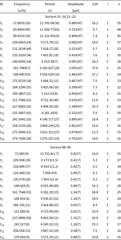
(TYC 770-941-1) was recognised as an sdB star from the LAMOST survey by Lei et al. (Reference Lei, Zhao, Németh and Zhao2018). The spectroscopic parameters reported by the authors and those we derived from a fit to our spectrum are listed in Table 1. Pulsations in this star were detected by Sahoo et al. (Reference Sahoo, Baran, Sanjayan and Ostrowski2020b). After the initial discovery of a significant signal in the long cadence (30 min) data, it was reobserved in the SC mode in Sectors 33 and 44–46. In the Sector 33 data, we detected 14 frequencies, out of which 11 were identified as dipole and two as quadrupole modes. We estimated an average period spacing of 232.59 (41) s and 134.29(24) s for dipole and quadrupole modes, respectively. In the combined Sectors 44–46 data, we detected 20 frequencies, out of which 13 were dipole and 5 were quadrupole modes. The average period spacings equals 235.7(8) s and 136.09(44) s for dipole and quadrupole modes, respectively. A difference between the average period spacings estimated in both two datasets are larger than their uncertainties. It is a consequence of some of the periods changed between datasets, which in turn, can be real and caused by the physical change of a pulsation cavity. In such cases, we consider period spacings and échelle diagrams separately. We list the frequencies in Table 3, plot amplitude spectrum in Fig. 2, and échelle diagrams in Fig. 3.
TIC 269766236
(Gaia DR2 6697530086799358720) was found to be a hot subdwarf candidate by Geier et al. (Reference Geier, Raddi, Gentile Fusillo and Marsh2019). A fit to our spectrum revealed that this star is hotter and more compact than a typical g-mode dominated sdB pulsator. The star was observed by TESS during Sector 27. We detected 11 pulsation frequencies, which are listed in Table 4. No rotationally split modes were found. Using an asymptotic period spacing we marked seven dipole and three quadrupole modes. Frequency
 $\mathrm{f}_{11}$
does not fit either dipole or quadrupole sequences, and we left it unidentified. We derived an average period spacing for dipole modes to be 241.0(6) s, and for quadrupole modes to be 139.15(35) s. We list the frequencies in Table 4, plot the amplitude spectrum in Fig. 4, and échelle diagrams in Fig. 5.
$\mathrm{f}_{11}$
does not fit either dipole or quadrupole sequences, and we left it unidentified. We derived an average period spacing for dipole modes to be 241.0(6) s, and for quadrupole modes to be 139.15(35) s. We list the frequencies in Table 4, plot the amplitude spectrum in Fig. 4, and échelle diagrams in Fig. 5.
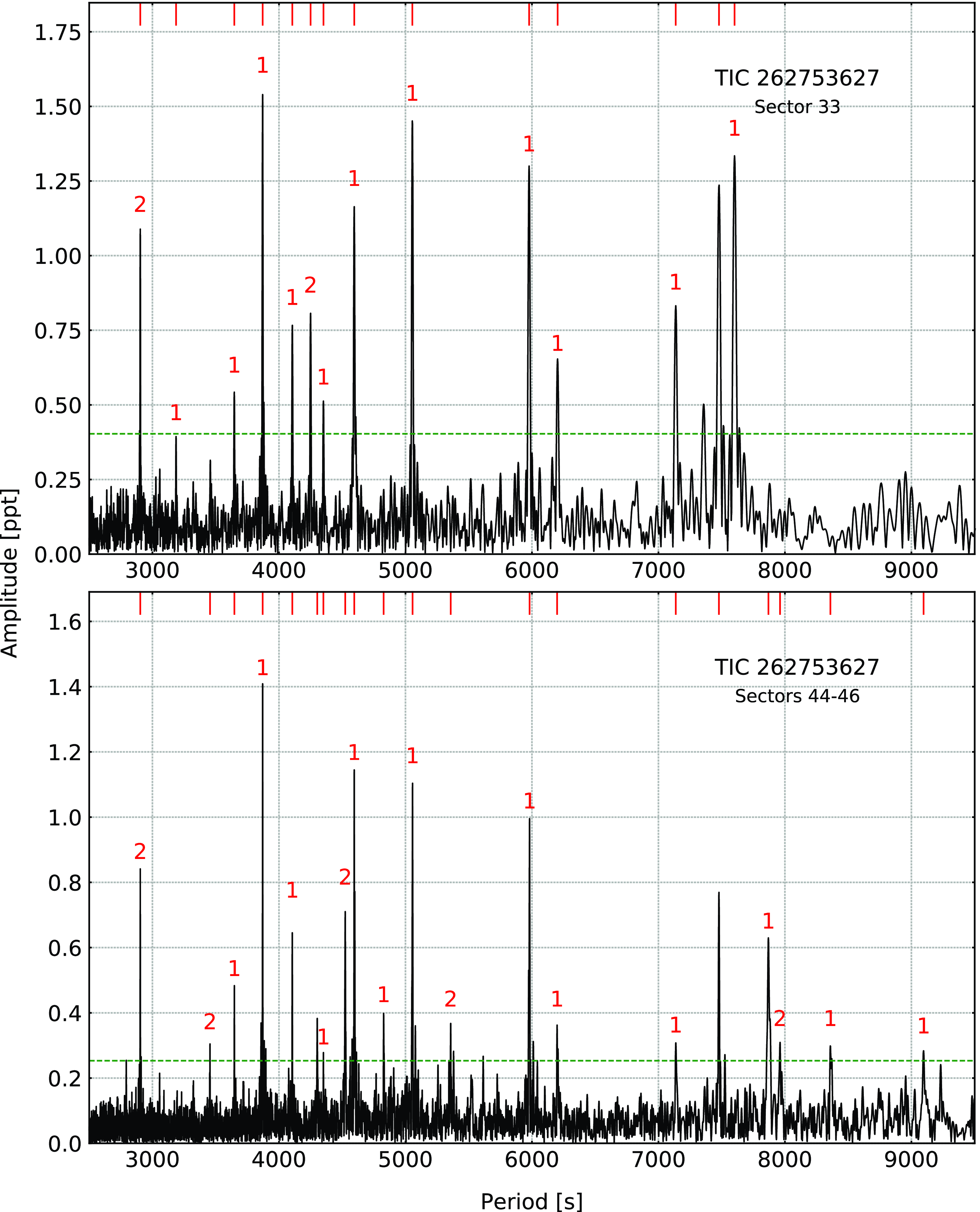
Figure 2. Amplitude spectra calculated from the SC data collected in different TESS sectors for TIC 262753627. The horizontal green dashed line denotes the detection threshold. Modal degrees are shown on top of each identified mode.
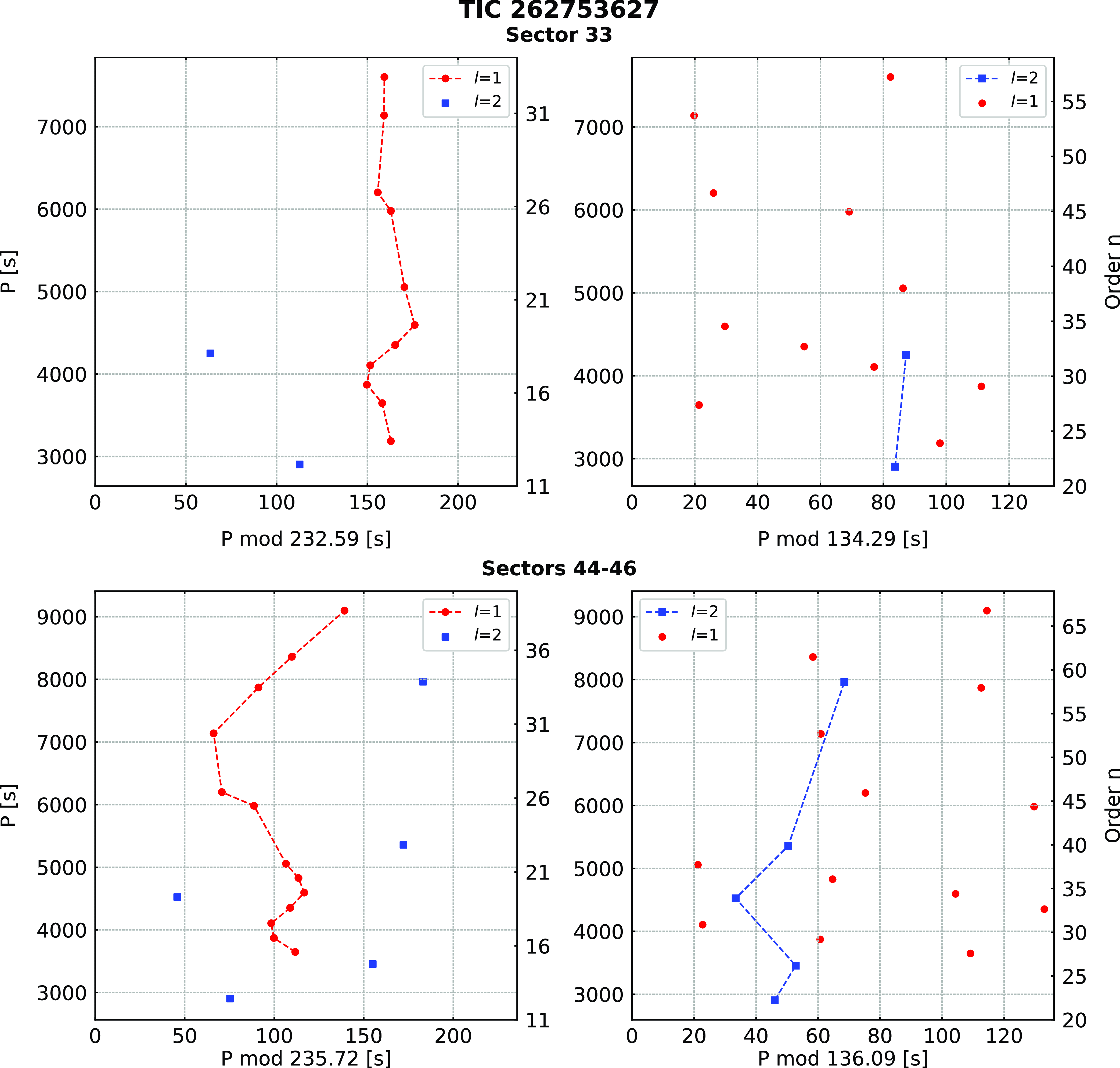
Figure 3. Échelle diagrams derived for SC data collected in different TESS sectors for TIC 262753627.
TIC 298109741
(PG 1340+607) was identified as an sdB star by Green et al. (Reference Green, Schmidt and Liebert1986). We confirm this spectral type with the spectroscopic parameters listed in Table 1. The star was observed by TESS during Sectors 15–16, 21–22, and 48–49. After examining each set individually, we combined Sector 15–16 and 21–22 data and prewhitened 19 frequencies in the range of 70–280
 $\mu$
Hz. No multiplets were found. We applied an asymptotic period spacing and identified 14 frequencies as dipole and 5 as quadrupole modes. We estimated an average period spacing for dipole modes to be 250.96(52) s, and for the quadrupole modes to be 144.89(30) s. We also combined the data from Sector 48–49 and detected 14 frequencies (12 dipole and 2 quadrupole modes). The average period spacings were within the uncertainties of the Sector 15–16 and 21–22 data. The average period spacings were 251.38(48) s for dipole and 145.13(28) s for quadrupole modes. A difference between the average period spacings is not significant, hence we calculated the average of those two values and used this value to calculate échelle diagrams for both datasets. The average period spacings calculated from all data equals 251.17(35) s and 145.01(21) s for dipole and quadrupole modes, respectively. We list the frequencies in Table 5, plot the amplitude spectra in Fig. 6, and échelle diagrams in Fig. 7.
$\mu$
Hz. No multiplets were found. We applied an asymptotic period spacing and identified 14 frequencies as dipole and 5 as quadrupole modes. We estimated an average period spacing for dipole modes to be 250.96(52) s, and for the quadrupole modes to be 144.89(30) s. We also combined the data from Sector 48–49 and detected 14 frequencies (12 dipole and 2 quadrupole modes). The average period spacings were within the uncertainties of the Sector 15–16 and 21–22 data. The average period spacings were 251.38(48) s for dipole and 145.13(28) s for quadrupole modes. A difference between the average period spacings is not significant, hence we calculated the average of those two values and used this value to calculate échelle diagrams for both datasets. The average period spacings calculated from all data equals 251.17(35) s and 145.01(21) s for dipole and quadrupole modes, respectively. We list the frequencies in Table 5, plot the amplitude spectra in Fig. 6, and échelle diagrams in Fig. 7.
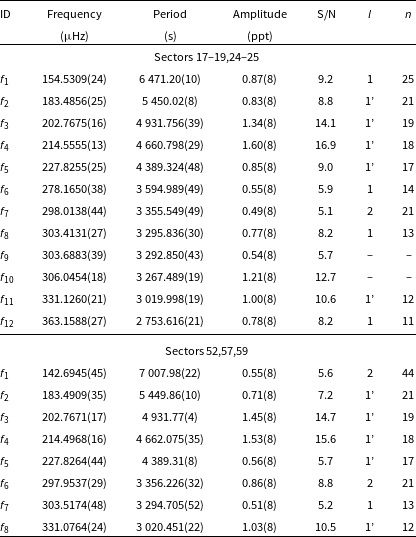
Table 6. Frequencies detected in amplitude spectra of TIC 311432346. An apostrophe sign denotes signals taken for analysis presented in Section 4.
TIC 311432346
(BD+29 3070) was listed as an sdOB+F star in the catalogue of hot subdwarfs (Kilkenny et al. Reference Kilkenny, Heber and Drilling1988). Spectroscopic parameters derived by Vos et al. (Reference Vos, Østensen, Németh, Green, Heber and Van Winckel2013) indicate the star to be an sdB with a main sequence companion. The star was observed by TESS during Sector 25–26 and 52–53. Our analysis of the Sector 25–26 data revealed 22 significant frequencies. The lowest frequency (near 7.74
 $\mu$
Hz) appears to have a strong first harmonic, and it can be interpreted either as binarity or the rotation of stellar spots on the main sequence companion. Since the amplitude of a flux variation is not stable over time we lean towards the latter explanation. The period of 1.49516(34) d, is quite different from the 1 283(63) days reported by Vos et al. (Reference Vos, Østensen, Németh, Green, Heber and Van Winckel2013). We detected 20 g-mode pulsations, but we found no multiplets. Using an asymptotic period spacing we identified 14 dipole and three quadrupole modes. We left two frequencies unidentified. The average period spacings are 254.87(38) s for dipole and 147.15(22) s for quadrupole modes, respectively. Our analysis of the Sectors 52–53 data revealed 14 frequencies, including two low frequencies discussed in the previous paragraph. Out of 12 pulsation frequencies, we identified nine as dipole modes, two as quadrupole modes. The average period spacings we calculated are 253.9(8) s and 146.61(43) s for dipole and quadrupole modes, respectively. The average period spacings calculated from all data equals 254.39(44) s for dipole and 146.88(24) s for quadrupole modes. We list the frequencies in Table 6, plot the amplitude spectra in Fig. 8, and échelle diagrams in Fig. 9.
$\mu$
Hz) appears to have a strong first harmonic, and it can be interpreted either as binarity or the rotation of stellar spots on the main sequence companion. Since the amplitude of a flux variation is not stable over time we lean towards the latter explanation. The period of 1.49516(34) d, is quite different from the 1 283(63) days reported by Vos et al. (Reference Vos, Østensen, Németh, Green, Heber and Van Winckel2013). We detected 20 g-mode pulsations, but we found no multiplets. Using an asymptotic period spacing we identified 14 dipole and three quadrupole modes. We left two frequencies unidentified. The average period spacings are 254.87(38) s for dipole and 147.15(22) s for quadrupole modes, respectively. Our analysis of the Sectors 52–53 data revealed 14 frequencies, including two low frequencies discussed in the previous paragraph. Out of 12 pulsation frequencies, we identified nine as dipole modes, two as quadrupole modes. The average period spacings we calculated are 253.9(8) s and 146.61(43) s for dipole and quadrupole modes, respectively. The average period spacings calculated from all data equals 254.39(44) s for dipole and 146.88(24) s for quadrupole modes. We list the frequencies in Table 6, plot the amplitude spectra in Fig. 8, and échelle diagrams in Fig. 9.
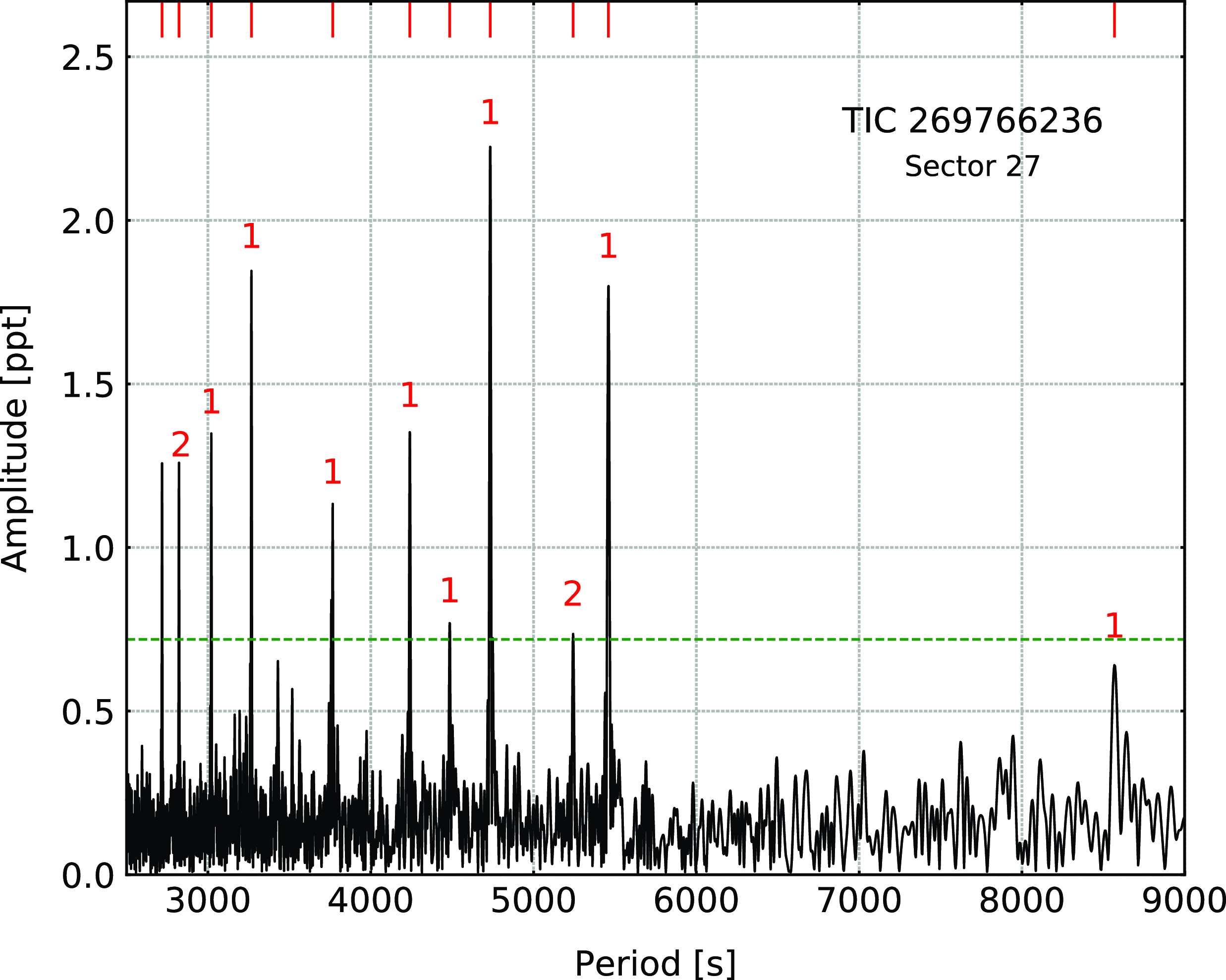
Figure 4. An amplitude spectrum for TIC 269766236. The horizontal green dashed line denotes the detection threshold. Modal degrees are shown on top of each identified mode.
TIC 331553315
(HS 0430+7712) was classified as an sdB star by Edelmann et al. (Reference Edelmann, Heber, Hagen, Lemke, Dreizler, Napiwotzki and Engels2003), and we list the spectroscopic parameters in Table 1. It was among 285 hot subdwarfs observed by Østensen et al. (Reference Østensen2010) using the Nordic Optical Telescope (NOT) but no variability was found. TESS observed the star during Sector 19, 25–26 52–53, and 59. After examining each set individually, we combined Sector 19 with Sectors 25–26 and detected 14 g-mode frequencies. By means of the asymptotic period spacing, we identified 11 dipole and three quadrupole modes. The average period spacings are 258.8(1.1) s and 149.4 (6) s for dipole and quadrupole modes, respectively. We found no rotationally split modes. From the combined Sector 52–53 and 59 data, we detected 12 frequencies, out of which we marked nine as dipole and three as quadrupole modes. The average period spacings are 257.7(2.0) s and 148.8(1.2) s for dipole and quadrupole modes, respectively. The average period spacings calculated from all data equals 258.3(1.1) s for dipole and 149.1(7) s for quadrupole modes. We list the frequencies in Table 7, plot amplitude spectra in Fig. 10 and échelle diagrams in Fig. 11.
TIC 367003034
(GALEX J223336.8+741254) was identified as an sdB star by Geier et al. (Reference Geier, Østensen, Nemeth, Gentile Fusillo, Gänsicke, Telting, Green and Schaffenroth2017); a fit to our spectrum confirms that identification. As with TIC 269766236, the fit results in a rather high surface gravity for a g-mode hot subdwarf. Boudreaux et al. (Reference Boudreaux2017) searched for pulsations in the GALEX data reporting a frequency of 7 891
 $\mu$
Hz. TESS observed the star during Sector 17–19, 24–25, 52, 57, and 59. We merged the Sector 17–19, 24–25 data and detected 12 g-mode frequencies. We found nine dipoles, one quadrupole, and one could not be defined. We estimated an average period spacing for dipole modes to be 266.8(1.8) s and for quadrupole modes to be 154.0(1.1). From the combined Sector 52, 57 and 59 data, we detected eight frequencies out of which we marked six as dipole and two as quadrupole modes. The average period spacings are 271.1(1.4) and 156.5(8) for dipole and quadrupole modes, respectively. We list the frequencies in Table 8, plot the amplitude spectra in Fig. 12 and échelle diagrams in Fig. 13.
$\mu$
Hz. TESS observed the star during Sector 17–19, 24–25, 52, 57, and 59. We merged the Sector 17–19, 24–25 data and detected 12 g-mode frequencies. We found nine dipoles, one quadrupole, and one could not be defined. We estimated an average period spacing for dipole modes to be 266.8(1.8) s and for quadrupole modes to be 154.0(1.1). From the combined Sector 52, 57 and 59 data, we detected eight frequencies out of which we marked six as dipole and two as quadrupole modes. The average period spacings are 271.1(1.4) and 156.5(8) for dipole and quadrupole modes, respectively. We list the frequencies in Table 8, plot the amplitude spectra in Fig. 12 and échelle diagrams in Fig. 13.
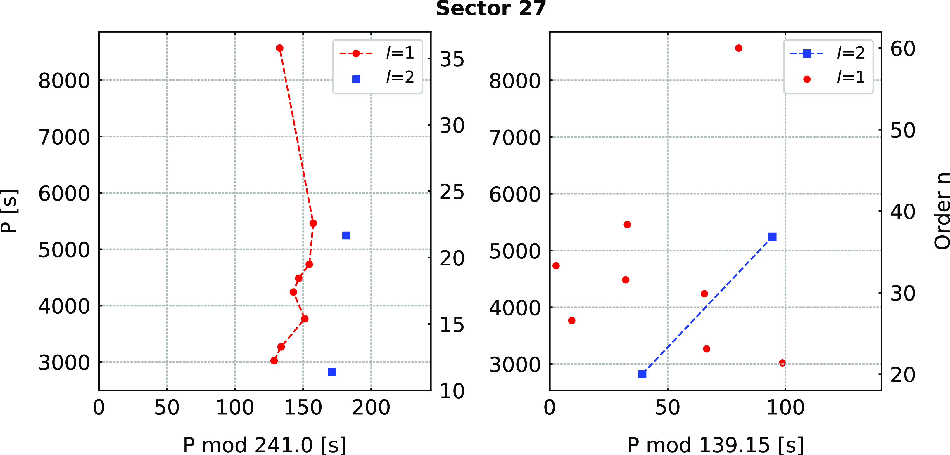
Figure 5. Échelle diagrams for TIC 269766236.
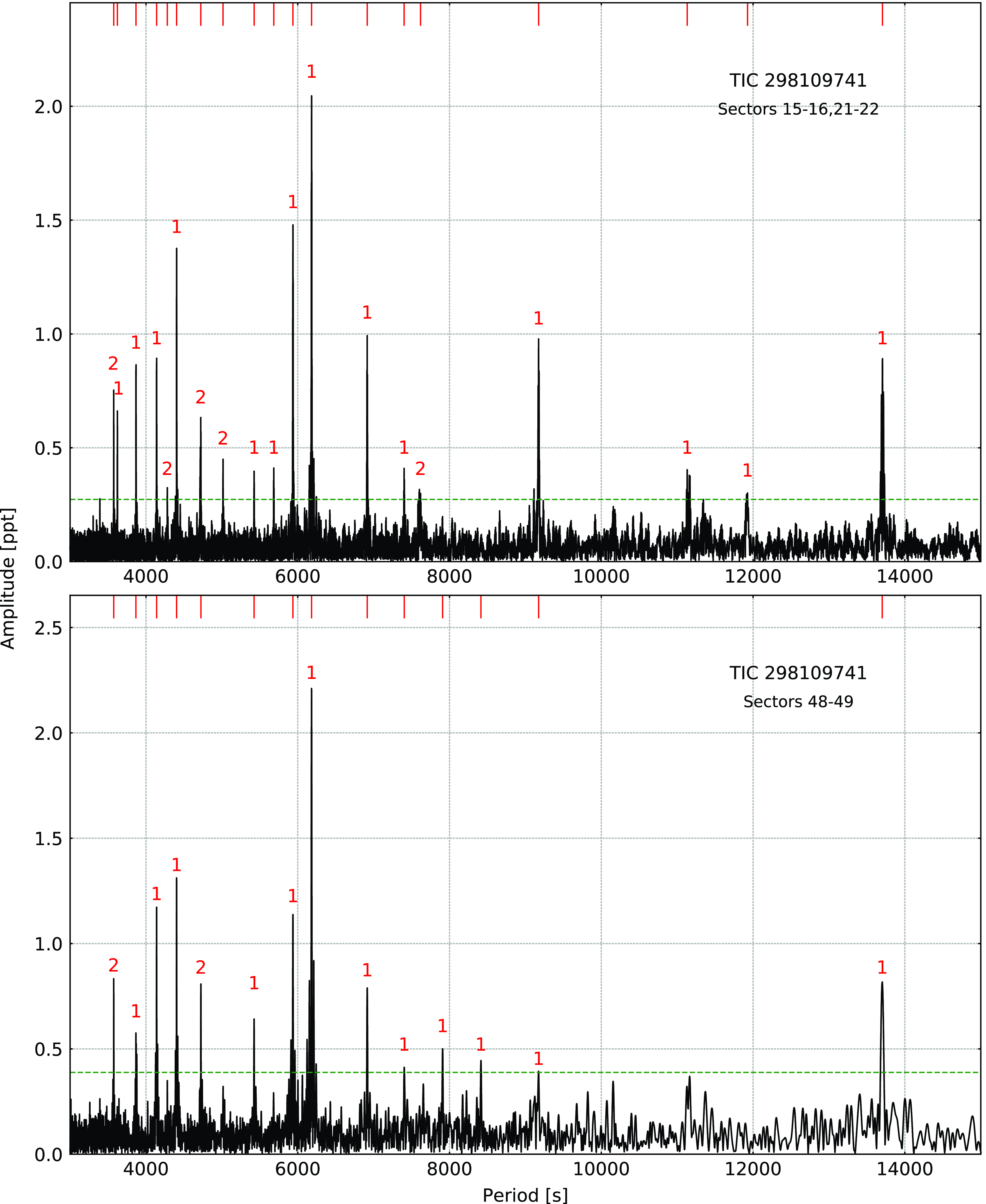
Figure 6. Amplitude spectra calculated from the SC data collected in different TESS sectors for TIC 298109741. The horizontal green dashed line denotes the detection threshold. Modal degrees are shown on top of each identified mode.
Table 7. Frequencies detected in amplitude spectra of TIC 331553315. An apostrophe sign denotes signals taken for analysis presented in Section 4.
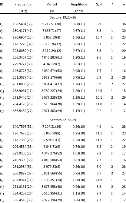
Table 8. Frequencies detected in amplitude spectra of TIC 367003034. An apostrophe sign denotes signals taken for analysis presented in Section 4.
4. Period fitting
A grid of evolutionary models was calculated using the publicly available and open-source code MESA (Paxton et al. Modules for Experiments in Stellar Astrophysics; Reference Paxton2019, version 11701). A detailed description of the physics and algorithms applied to calculate the models can be found in Ostrowski et al. (Reference Ostrowski, Baran, Sanjayan and Sahoo2021) which thoroughly explored MESA models of sdB stars. Newer versions of MESA do not contain any significant improvement in calculating both low to intermediate-mass main sequence and helium-burning EHB stars.
The models were calculated for progenitors with masses in the range 1.0–1.8 M
 $_\odot$
with 0.005 M
$_\odot$
with 0.005 M
 $_\odot$
step and metallicities, Z, in the range 0.005–0.035 with 0.005 step. The progenitors evolved to the tip of the red-giant branch where most of the hydrogen has been removed before the helium ignition, leaving only a residual hydrogen envelope on top of the helium core. The envelope masses,
$_\odot$
step and metallicities, Z, in the range 0.005–0.035 with 0.005 step. The progenitors evolved to the tip of the red-giant branch where most of the hydrogen has been removed before the helium ignition, leaving only a residual hydrogen envelope on top of the helium core. The envelope masses,
 $\mathrm{M}_\mathrm{env}$
, are in the range 0.0001–0.0030 M
$\mathrm{M}_\mathrm{env}$
, are in the range 0.0001–0.0030 M
 $_\odot$
with 0.0001 M
$_\odot$
with 0.0001 M
 $_\odot$
step, and in the range 0.003–0.010 M
$_\odot$
step, and in the range 0.003–0.010 M
 $_\odot$
with 0.001 M
$_\odot$
with 0.001 M
 $_\odot$
step. The models were relaxed to an equilibrium state and evolved until the depletion of helium in the core.
$_\odot$
step. The models were relaxed to an equilibrium state and evolved until the depletion of helium in the core.
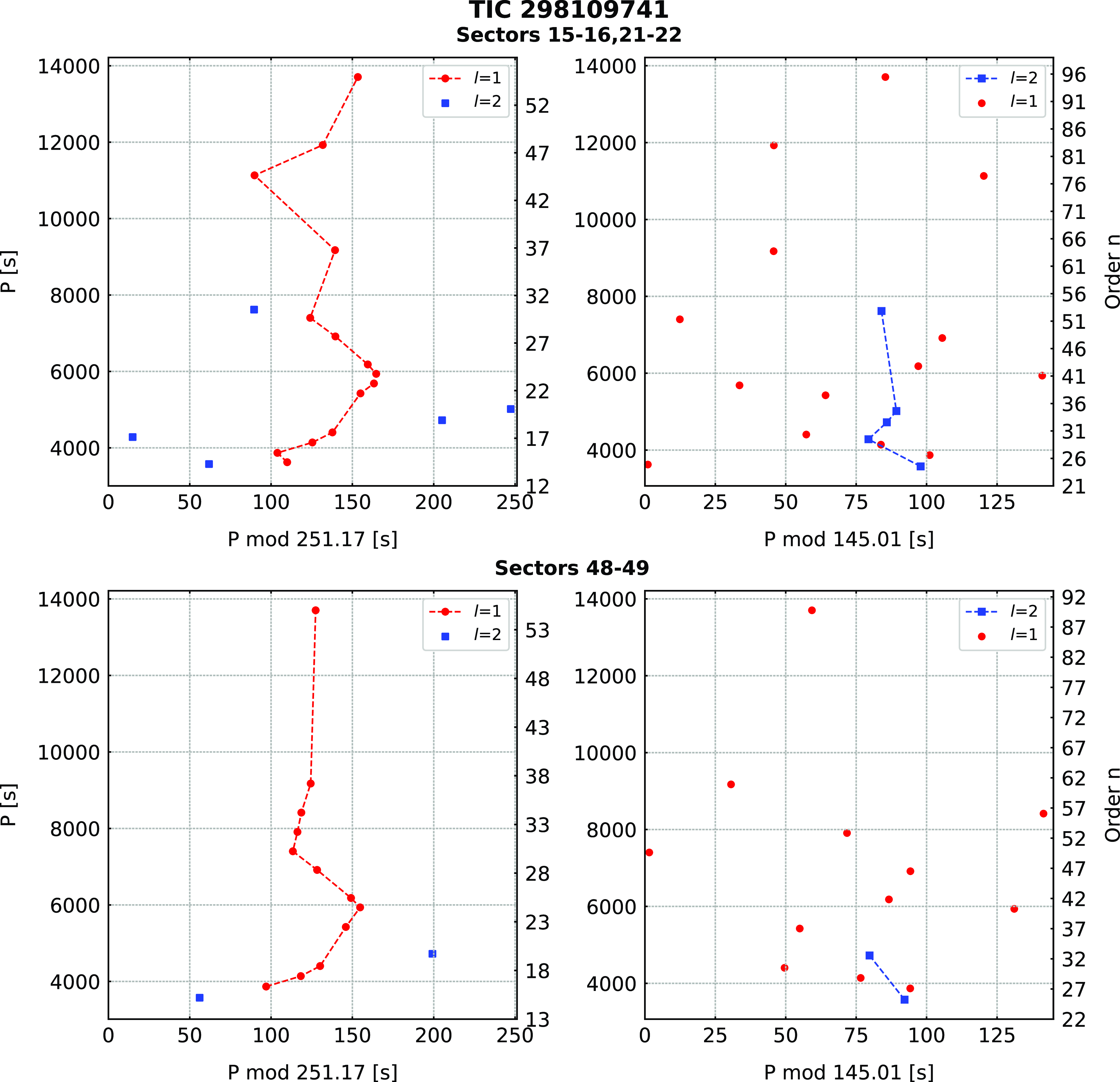
Figure 7. Échelle diagrams for TIC 298109741.
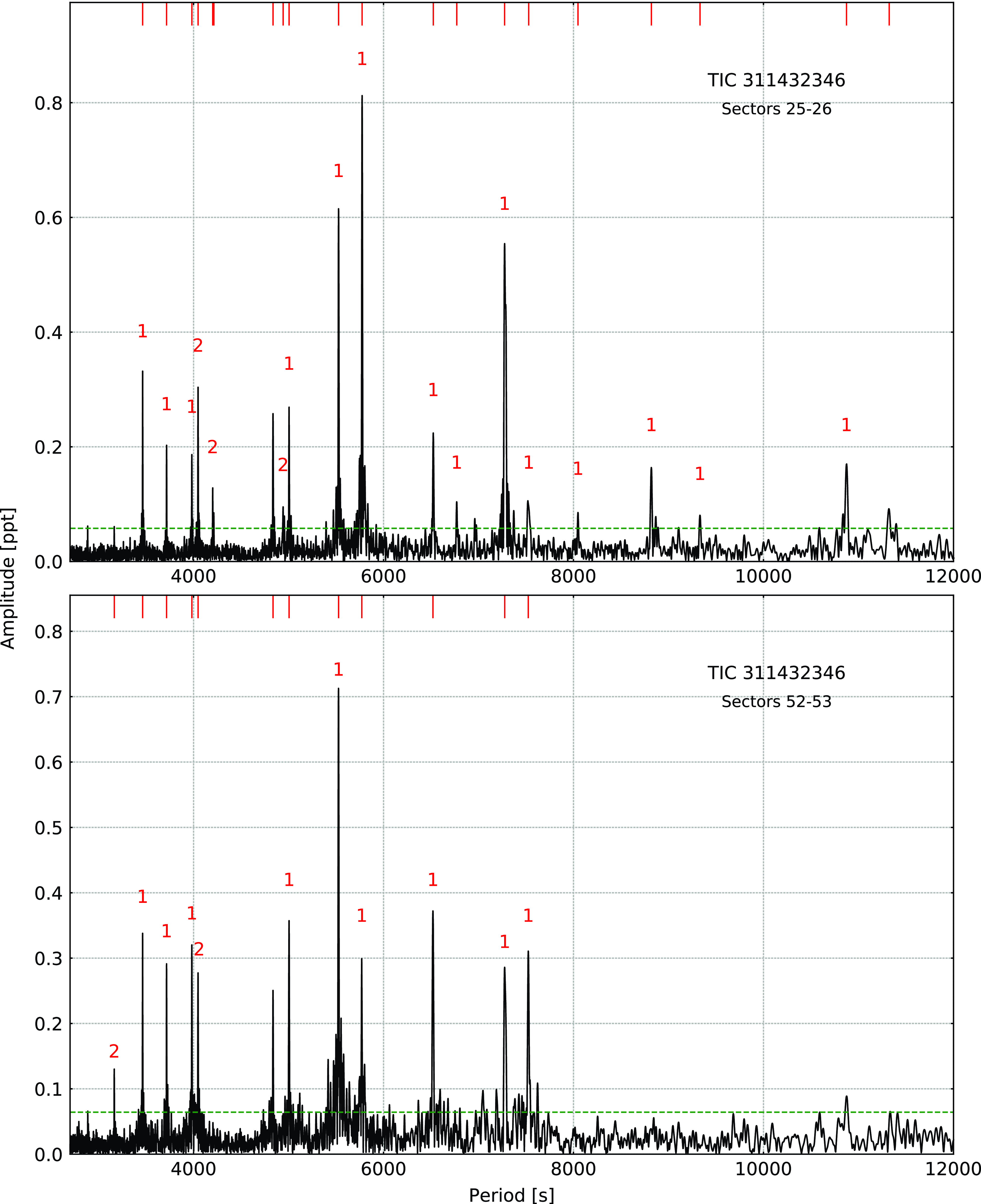
Figure 8. Amplitude spectra calculated from the SC data collected in different TESS sectors for TIC 311432346. The horizontal green dashed line denotes the detection threshold. Modal degrees are shown on top of each identified mode.
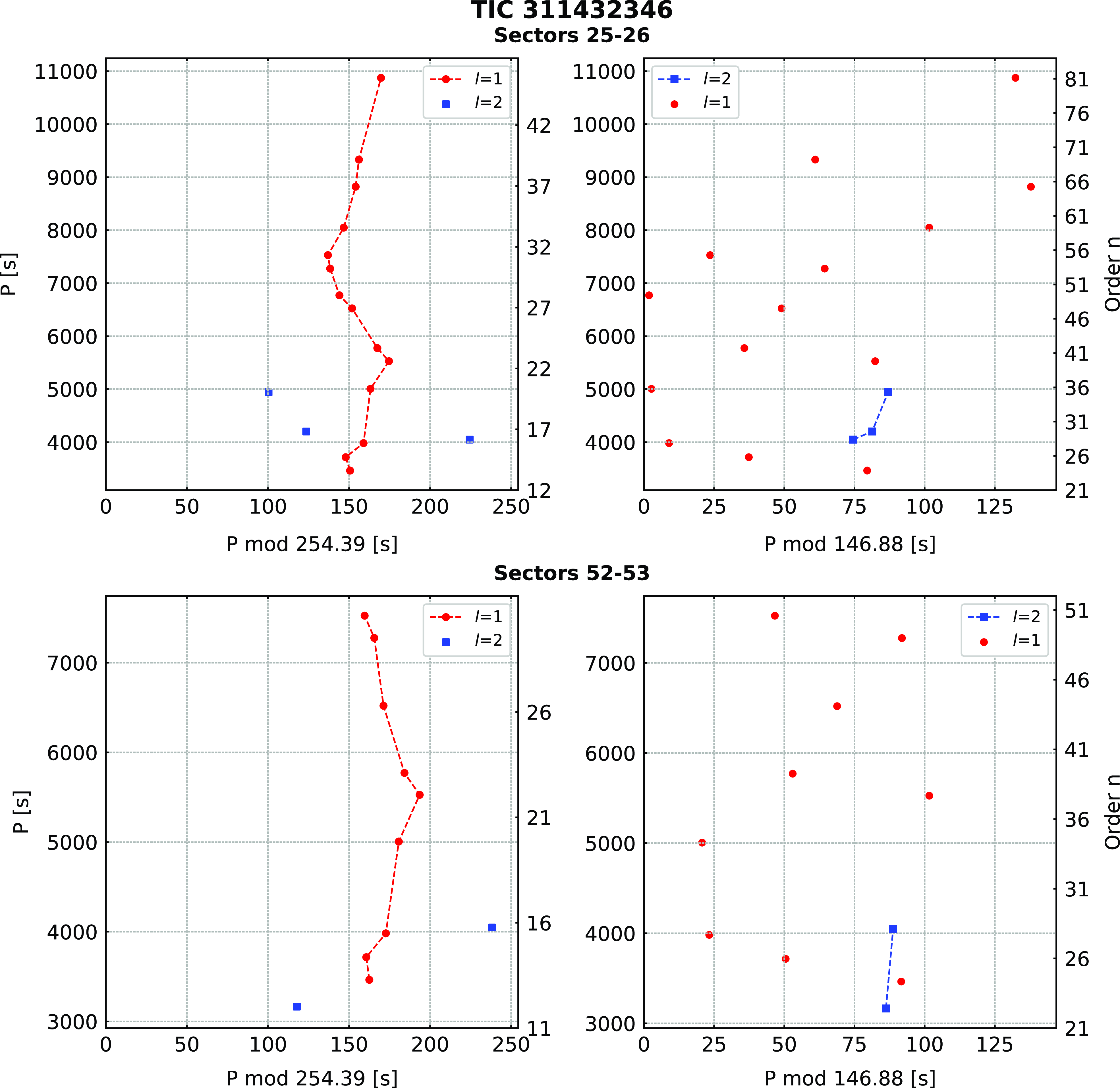
Figure 9. Échelle diagrams for TIC 311432346.

Figure 10. Amplitude spectra calculated from the SC data collected in different TESS sectors for TIC 331553315. The horizontal green dashed line denotes the detection threshold. Modal degrees are shown on top of each identified mode.

Figure 11. Échelle diagrams for TIC 331553315.
The adiabatic pulsation models were calculated using the GYRE code, version 5.2 (Goldstein and Townsend Reference Goldstein and Townsend2020). The pulsation models were calculated for evolutionary models with central helium abundance,
 $\mathrm{Y}_{\mathrm{c}}$
, in the range 0.9–0.1 with 0.05 increments. The models with
$\mathrm{Y}_{\mathrm{c}}$
, in the range 0.9–0.1 with 0.05 increments. The models with
 $\mathrm{Y}_{\mathrm{c}}$
< 0.1 were not considered because of the occurrence of the breathing pulses, which are currently an unavoidable side effect of using the convective premixing scheme (Ostrowski et al. Reference Ostrowski, Baran, Sanjayan and Sahoo2021).
$\mathrm{Y}_{\mathrm{c}}$
< 0.1 were not considered because of the occurrence of the breathing pulses, which are currently an unavoidable side effect of using the convective premixing scheme (Ostrowski et al. Reference Ostrowski, Baran, Sanjayan and Sahoo2021).
The calculated grid consists of 63 113 models with pulsation modes calculated up to a modal degree of l = 4. We used a goodness-of-fit function, which delivers a difference between observed and calculated periods:
 \begin{align*}{S}^2=\frac{1}{{N}_{o}}\,\sum^{{N}_{o}}_{i=1} \left({P}_{ o}^{{i}}-{P}_{c}^{{i}}\right)^2,\end{align*}
where
 $\mathrm{P}_{\mathrm{o}}$
is an observed period,
$\mathrm{P}_{\mathrm{o}}$
is an observed period,
 $\mathrm{P}_{\mathrm{c}}$
is a calculated period, and
$\mathrm{P}_{\mathrm{c}}$
is a calculated period, and
 $\mathrm{N}_{\mathrm{o}}$
is the number of periods used. The smallest
$\mathrm{N}_{\mathrm{o}}$
is the number of periods used. The smallest
 $\mathrm{S}^2$
value indicates the best fit. For our consideration, we accepted all fits up to 1.5 times the minimum value of
$\mathrm{S}^2$
value indicates the best fit. For our consideration, we accepted all fits up to 1.5 times the minimum value of
 $\mathrm{S}^2$
.
$\mathrm{S}^2$
.
To find the best fit between the models and observations, we adopted the following approach. We applied spectroscopic estimates of
 $\mathrm{T}_\mathrm{eff}$
and
$\mathrm{T}_\mathrm{eff}$
and
 $\log\,\mathrm{g}$
(listed in Table 1) and searched the grid of models within three times the uncertainties of both parameters. For TIC 262753627, Table 1 lists two different sets of estimates of spectroscopic parameters, however for the period fitting we adopted only the values derived in this paper. Since our calculated periods are based on adiabatic calculations we used preliminary mode identifications derived in this work. As explained earlier only an asymptotic period spacing was used, which makes the mode identification not necessarily correct. We limited our selection to dipole modes only, and the most convincing periods, that is, high amplitude and/or those detected in both datasets we analysed. For stars with two datasets collected during different Years of the TESS mission, we derived independent solutions for each dataset to check if they are sector-independent. Results of our period fitting are listed in Table 9. There are several caveats, our model tracks cover only core helium fusion, so the core helium fraction will always be > 0, which also places an upper limit on their ages. Also, as explained by Baran and Sanjayan (Reference Baran and Sanjayan2023), that is,
$\log\,\mathrm{g}$
(listed in Table 1) and searched the grid of models within three times the uncertainties of both parameters. For TIC 262753627, Table 1 lists two different sets of estimates of spectroscopic parameters, however for the period fitting we adopted only the values derived in this paper. Since our calculated periods are based on adiabatic calculations we used preliminary mode identifications derived in this work. As explained earlier only an asymptotic period spacing was used, which makes the mode identification not necessarily correct. We limited our selection to dipole modes only, and the most convincing periods, that is, high amplitude and/or those detected in both datasets we analysed. For stars with two datasets collected during different Years of the TESS mission, we derived independent solutions for each dataset to check if they are sector-independent. Results of our period fitting are listed in Table 9. There are several caveats, our model tracks cover only core helium fusion, so the core helium fraction will always be > 0, which also places an upper limit on their ages. Also, as explained by Baran and Sanjayan (Reference Baran and Sanjayan2023), that is,
 $T_\mathrm{eff}$
and
$T_\mathrm{eff}$
and
 $\log\,g$
are subject to large uncertainties, and only adiabatic pulsation periods were considered. Therefore, our period fitting solutions should be taken with caution.
$\log\,g$
are subject to large uncertainties, and only adiabatic pulsation periods were considered. Therefore, our period fitting solutions should be taken with caution.
TIC 262753627
We separately fitted periods detected in Sectors 33 and 44–46. All periods used are similar except for the longest period in each dataset. We obtained quite consistent solutions within individual and across the two datasets. The results show that this is a 0.47 M
 $_\odot$
star, with a radius of either 0.21 or 0.22 R
$_\odot$
star, with a radius of either 0.21 or 0.22 R
 $_\odot$
, which came from a progenitor of either 1.7 or 1.75 M
$_\odot$
, which came from a progenitor of either 1.7 or 1.75 M
 $_\odot$
. It still has 70% helium in its core, hence it has only been an EHB object for about 30 Myr. The envelope mass is around 0.0027 M
$_\odot$
. It still has 70% helium in its core, hence it has only been an EHB object for about 30 Myr. The envelope mass is around 0.0027 M
 $_\odot$
, while the mass of the convective core is 0.15 M
$_\odot$
, while the mass of the convective core is 0.15 M
 $_\odot$
. For a given progenitor mass there are a few solutions differing in envelope mass. This indicates that period fitting does not constrain the envelope mass particularly well and that small variations in both progenitor mass and envelope mass may deliver comparable sets of calculated pulsation periods.
$_\odot$
. For a given progenitor mass there are a few solutions differing in envelope mass. This indicates that period fitting does not constrain the envelope mass particularly well and that small variations in both progenitor mass and envelope mass may deliver comparable sets of calculated pulsation periods.
TIC 269766236
The best solutions constrained by spectroscopic estimates are listed in Table 9. The results show that this is a 0.47 M
 $_\odot$
star with a radius of either 0.20 or 0.21 R
$_\odot$
star with a radius of either 0.20 or 0.21 R
 $_\odot$
, which came from a progenitor of either 1.60 or 1.65 M
$_\odot$
, which came from a progenitor of either 1.60 or 1.65 M
 $_\odot$
. It has 0.45% helium in its core, which corresponds to about 70 Myr age since Zero Age Extreme Horizontal Branch (ZAEHB). The envelope mass is 0.0006 M
$_\odot$
. It has 0.45% helium in its core, which corresponds to about 70 Myr age since Zero Age Extreme Horizontal Branch (ZAEHB). The envelope mass is 0.0006 M
 $_\odot$
, on average, while the mass of the convective core is 0.14 M
$_\odot$
, on average, while the mass of the convective core is 0.14 M
 $_\odot$
.
$_\odot$
.
TIC 298109741
For both datasets, we derived only one and the same spectroscopically constrained solution, which meets the 1.5 S
 $^2$
criterion. The star is a 0.48 M
$^2$
criterion. The star is a 0.48 M
 $_\odot$
and 0.20 R
$_\odot$
and 0.20 R
 $_\odot$
hot subdwarf. It came from a 1.00 M
$_\odot$
hot subdwarf. It came from a 1.00 M
 $_\odot$
main sequence star. It still has 0.45 of the central helium to burn, which makes it almost 65 Myr old EHB star. The hydrogen envelope mass is 0.0007 M
$_\odot$
main sequence star. It still has 0.45 of the central helium to burn, which makes it almost 65 Myr old EHB star. The hydrogen envelope mass is 0.0007 M
 $_\odot$
, while its convective core is 0.15 M
$_\odot$
, while its convective core is 0.15 M
 $_\odot$
.
$_\odot$
.
TIC 311432346
Even though the uncertainty in
 $\mathrm{T}_\mathrm{eff}$
is quite large we found only three spectroscopic solutions satisfying the 1.5 S
$\mathrm{T}_\mathrm{eff}$
is quite large we found only three spectroscopic solutions satisfying the 1.5 S
 $^2$
criterion in Sectors 25–26 and two solutions in Sectors 52–53. The solutions are very similar and point to a 0.48 M
$^2$
criterion in Sectors 25–26 and two solutions in Sectors 52–53. The solutions are very similar and point to a 0.48 M
 $_\odot$
hot subdwarf with a radius of 0.19 M
$_\odot$
hot subdwarf with a radius of 0.19 M
 $_\odot$
, which is a descendant of a 1.35–1.50 M
$_\odot$
, which is a descendant of a 1.35–1.50 M
 $_\odot$
main sequence star. Based on the central helium, it is half way through the EHB stage (60 Myr). It has a hydrogen envelope mass of either 0.0011 or 0.0012 M
$_\odot$
main sequence star. Based on the central helium, it is half way through the EHB stage (60 Myr). It has a hydrogen envelope mass of either 0.0011 or 0.0012 M
 $_\odot$
, while the mass of the convective core is 0.15 M
$_\odot$
, while the mass of the convective core is 0.15 M
 $_\odot$
.
$_\odot$
.
TIC 331553315
This is the only star for which solutions derived from data collected over different cycles, were not closely similar. Instead, the best solutions indicate two possible models with either 0.20 or 0.45 of the central helium. This makes the star either 66 or 110 Myr old EHB object. The mass of the convective core is similar in both solutions – 0.14 or 0.15 M
 $_\odot$
. The total mass is 0.47 M
$_\odot$
. The total mass is 0.47 M
 $_\odot$
, while the size ranges between 0.18 and 0.24 R
$_\odot$
, while the size ranges between 0.18 and 0.24 R
 $_\odot$
. It has evolved from a main sequence progenitor with a mass between 1.70 and 1.80 M
$_\odot$
. It has evolved from a main sequence progenitor with a mass between 1.70 and 1.80 M
 $_\odot$
, while the possible mass of the hydrogen envelope lies between 0.0003 and 0.0026 M
$_\odot$
, while the possible mass of the hydrogen envelope lies between 0.0003 and 0.0026 M
 $_\odot$
.
$_\odot$
.
TIC 367003034
We derived only one and the same spectroscopically constrained solution for both datasets. The star is a 0.48 M
 $_\odot$
and 0.20 R
$_\odot$
and 0.20 R
 $_\odot$
hot subdwarf. It evolved from a 1.00 M
$_\odot$
hot subdwarf. It evolved from a 1.00 M
 $_\odot$
main sequence star. It still has 0.30 of the central helium to burn, which makes it an almost 85 Myr old EHB star. The hydrogen envelope mass is 0.0006 M
$_\odot$
main sequence star. It still has 0.30 of the central helium to burn, which makes it an almost 85 Myr old EHB star. The hydrogen envelope mass is 0.0006 M
 $_\odot$
while its convective core is 0.15 M
$_\odot$
while its convective core is 0.15 M
 $_\odot$
. This star is very similar to TIC 298109741.
$_\odot$
. This star is very similar to TIC 298109741.
5. Discussion
We aimed to investigate how pulsation modes in hot subdwarfs are related to the helium content and Galactic populations (thin disc, thick disc, halo). We collected a list of 1 587 hot subdwarfs and the relevant information from Luo et al. (Reference Luo, Németh, Wang, Wang and Han2021) and matched the list with the TESS database to retrieve TIC numbers. We found that 40 TIC targets have two different designations in the LAMOST database caused by close stars, and we kept those LAMOST identifiers that were closer to the positions in the Gaia DR3 catalogue (Gaia Collaboration et al. Reference Collaboration2023). This resulted in 1 547 targets. We used a list of 330 pulsating hot subdwarfs that we either collected from the literature or found in the TESS data up to Sector 60. We found that 46 pulsators are included in Luo et al. (Reference Luo, Németh, Wang, Wang and Han2021), while
 $T_\mathrm{eff}$
and helium content for another 30 pulsators we found in the SIMBAD database. In total, we collected the necessary data for 1 577 hot subdwarfs, including 76 (out of 330) pulsators.
$T_\mathrm{eff}$
and helium content for another 30 pulsators we found in the SIMBAD database. In total, we collected the necessary data for 1 577 hot subdwarfs, including 76 (out of 330) pulsators.

Figure 12. Amplitude spectra calculated from the SC data collected in different TESS sectors for TIC 367003034. The horizontal green dashed line denotes the detection threshold. Mode degrees are shown on top of each identified mode.
Figure 17 of Luo et al. (Reference Luo, Németh, Wang, Wang and Han2021) shows the helium content in hot subdwarfs. We extend that figure, for the first time, to show the relation between the helium content and the observed pulsations (Fig. 14). The majority of the pulsators are helium-poor hot subdwarfs including six pulsating subdwarf B stars reported in this paper, while we found no pulsators among the extremely helium-rich hot subdwarfs. We noticed that g-mode pulsators tend to be helium-poor, while p-mode pulsators can be both helium-poor and -weak. According to Figure 1 in Luo et al. (Reference Luo, Németh, Wang, Wang and Han2021), as
 $\mathrm{T}_\mathrm{eff}$
increases helium becomes more abundant in the atmosphere, so it should be no surprising that g-mode pulsators, which are on the lower
$\mathrm{T}_\mathrm{eff}$
increases helium becomes more abundant in the atmosphere, so it should be no surprising that g-mode pulsators, which are on the lower
 $\mathrm{T}_\mathrm{eff}$
end, do not show too much helium in the atmosphere. Three out of four iHe are g-mode pulsators, even though their temperature is well above 30 000 K. These pulsators belong to the group of heavy-metal subdwarfs that show unusual enrichment of elements such as zirconium and lead in their atmospheres. Perhaps this enrichment helps them to pulsate in g-modes even at higher temperatures.
$\mathrm{T}_\mathrm{eff}$
end, do not show too much helium in the atmosphere. Three out of four iHe are g-mode pulsators, even though their temperature is well above 30 000 K. These pulsators belong to the group of heavy-metal subdwarfs that show unusual enrichment of elements such as zirconium and lead in their atmospheres. Perhaps this enrichment helps them to pulsate in g-modes even at higher temperatures.
We derived space velocities (U, V, and W), orbital angular momentum (
 $\mathrm{L}_{\mathrm{z}}$
), and orbital eccentricity (e) for 96 pulsators, and modelled Galactic orbits using the Galpy python framework (Bovy 2015). The astrometric data (positions, distances, and proper motions) were collected from the Gaia DR3 database. We followed Altmann et al. (Reference Altmann, Edelmann and de Boer2004) and Luo et al. (Reference Luo, Németh, Wang, Wang and Han2021) in determining the Galactic population memberships of our 96 pulsating hot subdwarfs. Memberships of additional 1 547 hot subdwarfs, including 46 pulsators, were taken from Luo et al. (Reference Luo, Németh, Wang, Wang and Han2021).
$\mathrm{L}_{\mathrm{z}}$
), and orbital eccentricity (e) for 96 pulsators, and modelled Galactic orbits using the Galpy python framework (Bovy 2015). The astrometric data (positions, distances, and proper motions) were collected from the Gaia DR3 database. We followed Altmann et al. (Reference Altmann, Edelmann and de Boer2004) and Luo et al. (Reference Luo, Németh, Wang, Wang and Han2021) in determining the Galactic population memberships of our 96 pulsating hot subdwarfs. Memberships of additional 1 547 hot subdwarfs, including 46 pulsators, were taken from Luo et al. (Reference Luo, Németh, Wang, Wang and Han2021).
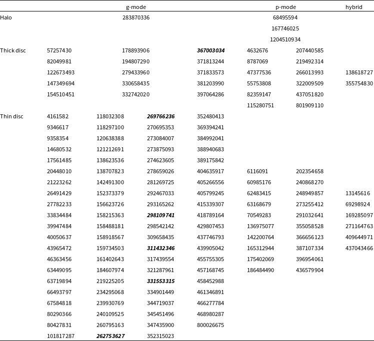
We allocated g-mode, p-mode, and hybrid pulsators to three Galactic populations – thin disc, thick disc, and halo – and show the list of pulsator types in each group in Table 10. The majority of hot subdwarf pulsators belong to the thin and thick disc populations. This is not unexpected, given where the stars are typically born. The halo population is, therefore, more sparse, but it is not yet clear if this is real effect or a bias caused by a limited sample. Our sample is dominated by g-mode pulsators, however we found more p-mode pulsators in the halo population. We stress, however, that we derived Galactic population memberships only for about a third of all pulsating hot subdwarfs in our list and the ratio may change if the size of the sample is increased, and a given Galactic population may show no preference for a specific pulsation type.
6. Summary and discussion
We have presented the results of our analysis of six pulsating hot subdwarfs observed by TESS. We used only the SC data because the USC data provided no additional frequencies in the g-mode region and no p-mode frequencies were detected. Two stars, TIC 262753627 and TIC 367003034, were reported to be pulsators prior to the TESS mission, while TIC 269766236, TIC 298109741, TIC 311432346, and TIC 33155331 were not.
We collected new spectra for four stars, TIC 262753627, TIC 269766236, TIC 298109741, and TIC 367003034, and determined their spectroscopic parameters, that is,
 $T_\mathrm{eff}$
,
$T_\mathrm{eff}$
,
 $\log\,g$
and
$\log\,g$
and
 $\log$
(n(He)/n(H)). For TIC 262753627, TIC 311432346, and TIC 33155331, we cited the atmospheric parameters we found in the literature. We have two independent estimates for TIC 262753627, which turned out to be different within their uncertainties. For further analysis, we accepted the estimates derived from our work.
$\log$
(n(He)/n(H)). For TIC 262753627, TIC 311432346, and TIC 33155331, we cited the atmospheric parameters we found in the literature. We have two independent estimates for TIC 262753627, which turned out to be different within their uncertainties. For further analysis, we accepted the estimates derived from our work.
Except for TIC 269766236, TESS observed stars over multiple sectors. We analysed data collected during two different years (data collected over separate years are denoted as datasets) and used this opportunity to compare the pulsation content. Most of the frequencies we detected exist in two datasets, with a few exceptions. For each star we found between 10 and 20 frequencies that were interpreted as g-mode pulsations. For each dataset, we performed a multiplet search (with a null result) and a mode identification using an asymptotic period spacing. Consequently, we derived modal degrees, relative radial orders, and average period spacings for all stars and independently for each dataset. The modal degree assignment does not depend on a dataset, while the average spacing is only different for TIC 367003034. Identification of modes using only the asymptotic period spacing method is not ideal, and hence our mode identifications should be taken with caution. Detection of multiplets in our datasets might have made our mode identifications more robust. Non-detection of any multiplet in the frequency spectrum may be due to a large inclination of the star from the line of sight, a very slow rotation, so the splits of the frequency peaks are smaller than the resolution, or low amplitudes being below the detection threshold we applied.
Table 9. Models fitting the observed periods of dipole modes within 1.5 S
 $^2$
, and
$^2$
, and
 $T_\mathrm{eff}$
and
$T_\mathrm{eff}$
and
 $\log\,g$
within three times their uncertainties.
$\log\,g$
within three times their uncertainties.
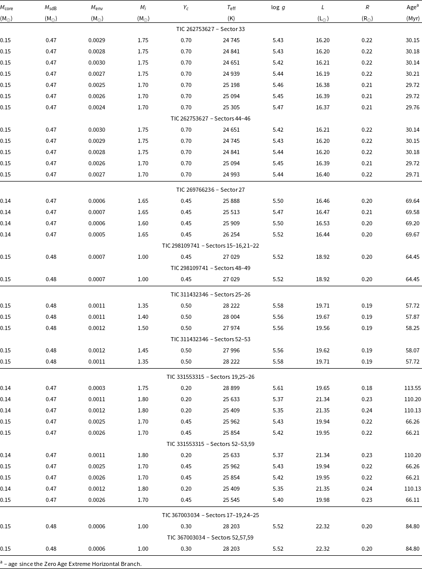

Figure 13. Échelle diagrams derived for TIC 367003034.

Figure 14. Helium content in function of effective temperature for hot subdwarfs. The four helium group ranges were taken from Luo et al. (Reference Luo, Németh, Wang, Wang and Han2021). The six g-mode rich pulsating subdwarfs that are discussed in this paper are shown with filled circles. Designations we used in the figure follow the ones in Luo et al. (Reference Luo, Németh, Wang, Wang and Han2021), that is, eHe – extreme He-rich, iHe – intermediate He-rich, wHe – He-weak, pHe – He-poor.
We used a grid of evolutionary and pulsation models calculated with the MESA and GYRE to derive the physical parameters of our stars by comparing the observed pulsation periods with the modelled ones. We defined a function
 $\mathrm{S}^2$
to compare the observed and calculated periods and normalised it by the number of periods used. This function was then used as a criterion to select pulsation models that best fit the observations. We restricted solutions to atmospheric parameters within three times their uncertainties to broaden the grid search and eliminate well-defined but accidental solutions. For each star we obtained either a unique solution or a set of solutions, which differ only slightly in input parameters. The only exception is the central helium content in TIC 331553315.
$\mathrm{S}^2$
to compare the observed and calculated periods and normalised it by the number of periods used. This function was then used as a criterion to select pulsation models that best fit the observations. We restricted solutions to atmospheric parameters within three times their uncertainties to broaden the grid search and eliminate well-defined but accidental solutions. For each star we obtained either a unique solution or a set of solutions, which differ only slightly in input parameters. The only exception is the central helium content in TIC 331553315.
We used a sample of 1 577 hot subdwarfs to check the relation between the helium content and pulsations. We found that no pulsators (out of 76) exist among the extremely rich helium hot subdwarfs, while the population of pulsators increases as the helium content decreases. We used a sample of 1 640 hot subdwarfs, including 142 pulsators, to check the distribution of pulsators across the Galactic populations. We found p- and g-mode pulsators in all Galactic populations. Since g-mode pulsators dominate our sample we expected these pulsators to be the most abundant in all populations, however, we found the Galactic halo contains more p-mode pulsators. The number of pulsators in the halo is very small so it may not be a real effect and this trend should be confirmed with a larger sample. This analysis is the first to use a set of pulsating subdwarfs to correlate the pulsation properties with the Galactic populations. A limited sample is the main caveat for such analyses at the moment.
Table 10. A list of 142 hot subdwarf pulsators allocated to their Galactic populations. The six pulsating subdwarfs presented in this paper are marked in bold and italic.
Acknowledgements
Financial support from the National Science Centre Poland under projects No. UMO-2017/26/E/ST9/00703 is acknowledged. P.N. acknowledges support from the Grant Agency of the Czech Republic (GAČR 22-34467S). The Astronomical Institute in Ondrřejov is supported by the project RVO:67985815. This paper uses observations made at the South African Astronomical Observatory (SAAO). This research has used the services of www.Astroserver.org. This research made use of Lightkurve, a Python package for Kepler and TESS data analysis (Lightkurve Collaboration et al. 2018).
Data availability
The data sets were derived from MAST in the public domain archive.stsci.edu.


