2.1. Extreme learning machine

As a variant of the ANN, the ELM does not require gradient-based backpropagation to adjust the weights but sets the weights through the Moore–Penrose generalized inverse [Reference Gilabert, Braithwaite and Montoro20]. The standard ELM neural network structure is shown in Fig. 1. For any $N$ samples $(x_i,t_i)$ , ${x_i} = [x_1^i,x_2^i, \cdots,x_n^i]^{\textrm{T}} \in{R^n}$ is the input vector of the $i$ sample, $n$ is the number of input layer nodes, ${t_i} = [t_1^i,t_2^i, \cdots,t_l^i]^{\textrm{T}} \in{R^l}$ , $l$ is the number of output layer nodes. The number of hidden layer nodes is $m$ , and the hidden layer activation function is $g(x)$ . Input weights $\omega$ , hidden layer thresholds $b$ , and output weights $\beta$ are $m \times n$ , $m \times 1$ , and $l \times m$ matrix, respectively. Then the mathematical model is as follows:

(1) \begin{equation}{t_k} = \sum \limits _{i = 1}^m{{\beta _i}{g_i}(\omega,b,{x_k})} = \sum \limits _{i = 1}^m{{\beta _i}{g_i}({\omega _i} \cdot{x_k} +{b_i}),(k = 1,2, \cdots,N)} \end{equation}

which $\omega _i$ is $1 \times n$ , the weights of the input layer nodes and the $i$ hidden layer node. $x _k$ is $n \times 1$ , the $i$ th input sample. $\beta _i$ is $l \times 1$ , the weights of the $i$ hidden layer node and the output layer nodes. $t _k$ is $l \times 1$ , output of the $i$ sample. The above $N$ equations can be abbreviated as:

(2) \begin{equation} H\beta = T \end{equation}

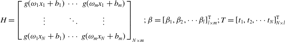(3) \begin{equation} H ={\left [{\begin{array}{*{20}{c}}{g({\omega _1}{x_1} +{b_1})}& \cdots &{g({\omega _m}{x_1} +{b_m})}\\[5pt] \vdots & \ddots & \vdots \\[5pt]{g({\omega _1}{x_N} +{b_1})}& \cdots &{g({\omega _m}{x_N} +{b_m})} \end{array}} \right ]_{N \times m}};\;\beta = \left [{{\beta _1},{\beta _2}, \cdots{\beta _l}} \right ]_{l \times m}^{\textrm{T}}\!;\; T = \left [{{t_1},{t_2}, \cdots{t_N}} \right ]_{N \times l}^{\textrm{T}} \end{equation}

$H$ is called the hidden layer output matrix, $\beta$ is the output layer weight matrix, and $T$ is the expected output. According to the least square norm solution of the above equation [Reference Chen, Lv, Lu and Dou21], it can be obtained that $\hat \beta ={H^\dagger }T$ , $H^\dagger$ is the generalized inverse matrix of $H$ .

Figure 1. ELM network structure diagram.

2.2. Kalman particle swarm optimization

The principle of Kalman filtering makes an optimal estimate of the final state by referring to the predicted and observed values [Reference Mo, Song, Li and Jiang22]. Specifically, given an observation $Z_{t + 1}$ , KPSO is used to generate a Gaussian distribution about the true state. The parameters $m_{t + 1}$ and $V_{t + 1}$ of this multivariate distribution are determined by the following equations:

(4) \begin{equation} {m_{t + 1}} = F{m_t} +{K_{t + 1}}({Z_{t + 1}} - GF{m_t}) \end{equation}

(5) \begin{equation} {V_{t + 1}} = (I -{K_{t + 1}})(F{V_t}{F^{\textrm{T}}} +{V_X}) \end{equation}

(6) \begin{equation} {K_{t + 1}} = (F{V_t}{F^{\textrm{T}}} +{V_X}){G^{\textrm{T}}}{(G(F{V_t}{F^{\textrm{T}}} +{V_X}){G^{\textrm{T}}} +{V_Z})^{ - 1}} \end{equation}

where $F$ and $V_X$ describe the system transition model and process noise, while $G$ and $V_Z$ describe the system sensor model and observation noise [Reference Peng, Chen and Yang23]. The best estimate of the true state results from a Gaussian distribution:

(7) \begin{equation} {x_t} \sim Normal({m_t},{V_t}) \end{equation}

KPSO prescribes particle changes entirely based on Kalman’s prediction principles. Every particle has its $m_t$ , $V_t$ , and $K_t$ . The particles then generate observations with the following equation:

(8) \begin{equation}{z_v} = \phi(g - x);\;\;\begin{array}{*{20}{c}}{} \end{array}{z_p} = x +{z_v};\;\;\begin{array}{*{20}{c}}{} \end{array}Z = (z_p^T,z_v^T) \end{equation}

where $\phi$ is uniformly extracted in the interval $[0.2, 0.5]$ . Then $m_t$ and $V_t$ are generated from the observations of Eqs. (4), (5), and (6). After the observations are determined, the optimal estimated state of the particle is obtained by Eq. (7). The new state of the particle is obtained by sampling this distribution, and the position information of particles is extracted from $x_{t + 1}$ . The system model parameters are set as follows, where $d$ is the individual dimension, and $o$ is the individual vector [Reference Xu, Chen and Yu17].

(9) \begin{equation} F = \left ({\begin{array}{*{20}{c}}{{I_d}}\;\;\;&{{I_d}}\\[5pt] 0\;\;\;&{{I_d}} \end{array}} \right )\!;\;{V_Z} = diag(o );\;{V_X} = diag(o);\;G ={I_{2d}} \end{equation}

3.1. KPSO using Cauchy distribution

Traditional KPSO uses complex computations when updating particle predictions and covariance matrices, which can be time-consuming in practical engineering applications. In this paper, KPSO is improved according to the calculation method of Kalman gain in ref. [Reference Wu, Liu, Guo, Shi and Xie19], and the Cauchy distribution is used to generate the optimal estimate. The Cauchy distribution has the characteristics of no expectation and no variance, and its probability density function is

(10) \begin{equation} f(x) = \frac{\beta }{{\pi \!\left [{{\beta ^2} +{{\left ({x - \alpha } \right )}^2}} \right ]}}\begin{array}{*{20}{c}}, \end{array}\beta \gt 0 \end{equation}

where $\alpha$ is the position parameter that defines the peak position of the distribution, and $\beta$ is the scale parameter that defines the half-width at half the maximum value. There are two reasons for using the Cauchy distribution function: (1) The existing KPSOs use a Gaussian distribution for optimal estimation, and the velocity information of particles is used as the covariance matrix of the distribution. However, the velocity information is directional, which does not meet the requirements of a positive definite covariance matrix, and the calculation is also complex; (2) When using the Cauchy distribution function to generate offspring, it has a certain probability of generating a mutation value. Due to the non-expectation and non-variance nature of the Cauchy distribution function, mutation value is allowed, which increases the diversity of the population in the search process and is more accommodating to search. In summary, when using Cauchy distribution to generate offspring, the diversity of the population is enhanced and the computational efficiency is improved.

3.2. Hierarchical division in KPSO search process

PSO was proposed by Eberhart and Kennedy in 1995 [Reference Sengupta, Basak and Peters24]. PSO is a swarm intelligence algorithm designed by simulating the predation behavior of birds. There are food sources of different sizes in the search space, and birds are tasked with finding the largest food source ( $gbest$ ). Birds in the search process, through mutual transmission of their information, cooperate to find the optimal solution. Essentially, PSO finds $gbest$ through an iterative process. In each iteration, each particle produces a new particle. The newly generated particles are called the offspring, and the original particles are called the parents.

In the early stages of PSO search, it is intended that the particles in the population will diverge as much as possible and enhance the global exploration capability. In the late search, particles need to convergence as much as possible to enhance their local exploitation ability. In the proposed algorithm, the distance between the parents and the offspring in each iteration is calculated, and the first $\left \lfloor{ W*N} \right \rfloor$ individuals are selected to be defined as the convergent state and the rest as the divergent state, where $W$ is the inertia weight, and $N$ is the population size. The individuals in the convergence state are modified to ensure the exploration and exploitation ability of the algorithm.

Algorithm 1: IKPSO

3.3. Overview of the proposed approach

The pseudo-code of the IKPSO is shown in Algorithm 1. Firstly, the PSO principle is used to generate the offspring $pops$ , and then the Euclidean distance $dis$ between $pops$ and $pop$ is calculated. Secondly, the population is divided into a convergence state and a divergence state according to the distance index, and the individuals in the convergence state are corrected by Kalman filtering. Finally, the number of the stagnations of $gbest$ is calculated. If the upper limit is reached, a Kalman filtering correction is performed on the entire population.

3.4. Fitness function

As mentioned above, the input weights $\omega$ and hidden layer thresholds $b$ of ELM are randomly set, and they cannot be guaranteed that the model has good robustness. Aiming at this problem, the artificial intelligence optimization algorithm is used to optimize the input weights and thresholds of ELM to improve the robustness of the model.

In this paper, the IKPSO algorithm is used to optimize $\omega$ and $b$ of ELM. Assuming that the number of input nodes of ELM is $n$ and the number of hidden layer nodes is $m$ , the individual dimension to be optimized is $(n+1)*m$ . An optimization individual can be represented as ${\alpha _i} = [{\omega _{11}},{\omega _{12}}, \cdots,{\omega _{1n}}, \cdots,{\omega _{mn}},{b_1}, \cdots,{b_m}]$ , $\alpha _i$ is the $i$ individual to be optimized, where ${\omega _{mn}} \in [\!-\!1,1]$ , ${b_m} \in [0,1]$ . The root mean square error (RMSE) function [Reference Liang, Guo, Yu, Qu, Yue and Qiao25] between the output value of the model and the target value is used as the fitness function, as shown in Eq. (11), which $fit({\alpha _i})$ is the fitness value of individual $\alpha _i$ , $N_{train}$ is the number of samples, and $Y_i$ and $f\!\left ({{\alpha _i}} \right )$ are the true value and model output value of the $i$ sample, respectively.

(11) \begin{equation} fit({\alpha _i}) = \sqrt{\frac{1}{{{N_{train}}}}\sum \limits _{i = 1}^{{N_{train}}}{{{\left ({{Y_i} - f\!\left ({{\alpha _i}} \right )} \right )}^2}} } \end{equation}

4.1. Experiment simulation and parameter setting

The experimental data come from a 300 MWe CFBB in China. There are a total of 20 operational parameters and 2 target parameters. A simplified CFBB model is shown in Fig. 2. Therefore, the number of input layer nodes of the ELM is 20, and the number of output layer nodes is 2. The number of hidden layer nodes is set to 80 by parameter verification, and the verification curve is shown in Fig. 3(a).

Figure 2. Simplified CFBB model.

Figure 3. Figures of the experimental results.

Figure 4. Simplified CFBB model.

In order to verify the optimization ability of the proposed IKPSO algorithm, it is compared with PSO [Reference Sengupta, Basak and Peters24], KPSO [Reference Peng, Chen and Yang23], OFA [Reference Zhu and Zhang26], and DE [Reference Zhu, Qin, Suganthan and Huang13] on the CEC2017 benchmark functions [Reference Awad, Ali, Liang, Qu and Suganthan27] in Section 4.2. All experiments are conducted 51 times independently, the dimension of the test functions is 100, the total number of evaluations is 1000000, and the population size is set to 100. The experimental results are verified by the Wilcoxon rank-sum test [Reference Derrac, García, Molina and Herrera28].

In Section 4.3, the proposed ELM based on IKPSO optimization (ELM-IKPSO) is compared with ELM [Reference Huang, Zhu and Siew10], ELM-PSO [Reference Han, Yao and Ling16], ELM-OFA [Reference Zhu and Zhang26], and ELM-DE [Reference Zhu, Qin, Suganthan and Huang13], respectively. The optimized ELM has the same parameters. Because the number of hidden layer nodes is set to 80, according to the fitness function setting in Section 3.4, the individual dimension to be optimized is $\alpha =1680$ . The total evaluation times of PSO, DE, OFA, and IKPSO are 80,000, and the population size is 100. The experiments are run independently 51 times and simulated on Python 3.9. In order to prevent model overfitting, the training data set is divided into a training set and a validation set, and the RMSE of the model on the validation set is taken as the optimization goal. The structure diagram of the data set division is shown in Fig. 4. Finally, the statistical test is performed by the Wilcoxon rank-sum test [Reference Derrac, García, Molina and Herrera28], and the confidence level $\alpha$ [Reference Liang, Zhang, Yu, Qu, Yue and Qiao29] is set to 0.05. Finally, the proposed method is used for multi-objective optimization on the established model to improve boiler thermal efficiency and reduce NOx emissions.

4.2. CEC2017 benchmark functions validation

In order to test the optimization ability of the algorithm using the Cauchy distribution, several evolutionary algorithms are compared on the CEC2017 benchmark functions. KPSO is the original algorithm using a Gaussian distribution function, and IKPSO is the improved algorithm using a Cauchy distribution function. Detailed experimental results are shown in Table I. The best results are shown in bold. It can be seen from the experimental results that the optimization ability of the algorithm is improved after using the Cauchy distribution function to generate the offspring, and IKPSO is superior to KPSO in all 30 test functions. The reason is that the use of Cauchy distribution to generate offspring can make the population find potential regions for development more quickly and make full use of computing resources. From the comparison of KPSO and IKPSO with PSO, it can be concluded that the algorithm using the Kalman filter principle improves the optimization ability of PSO. In addition, in comparison with other types of evolutionary algorithms, OFA and DE, IKPSO is superior to the compared algorithms in 23 and 20 functions, respectively. In summary, IKPSO is superior to the compared algorithms, showing stronger optimization ability and generalization performance.

Table I. Experimental results on the CEC2017 test functions.

4.3. Model establishment and analysis

The detailed results of the modeling algorithms are shown in Table II. As shown in Table II, a comparison of the outcome metrics for ELM, ELM-PSO, ELM-OFA, ELM-DE, and ELM-IKPSO is listed. For each algorithm, the best result is shown in bold font. For the training data, ELM-IKPSO has the smallest performance metric, significantly outperforming the compared algorithms. For the test data, it can be seen that although ELM-DE is similar to ELM-IKPSO in the minimum value, it is worse than ELM-IKPSO in both mean and variance, which proves that ELM-IKPSO has better robustness and generalization ability. Therefore, ELM-IKPSO has good generalization performance, and the model built by ELM-IKPSO is efficient. Figure 3(b) plots the boxplot of the five algorithms on the test set. From the information in the box diagram, ELM-IKPSO achieves better statistical results. In addition, the four optimized models are more obvious than the original ELM algorithm, which proves the importance of the optimized ELM.

Table II. Detailed RMSE results.

Figure 3(c) shows the iterative convergence diagram of different evolutionary algorithms in the optimization process, where the horizontal axis is the number of fitness function evaluations, and the vertical axis is the mean of the validation set results. It can be seen from the convergence curve that the OFA converges too fast, and it is easy to converge to the local optimum in the CFBB modeling problem. DE and PSO are better than OFA. After using the Kalman filter principle to correct PSO, the extra number of fitness evaluations will be consumed in each iteration to find more potential regions and prevent convergence to the local optimum. From the perspective of the search process, the IKPSO algorithm is superior to the compared algorithms. Figure 3(d) and (e) shows the fitting effect on the test set. Figure 3(d) shows the thermal efficiency fitting effect, and Fig. 3(e) shows the NOx fitting effect. The blue star marks the actual data. In addition, it can be seen from the two simulation graphs that the output values of ELM-IKPSO are close to the actual data. The model built by ELM-IKPSO is efficient.

Finally, the established model is multi-objective optimized to increase the boiler combustion efficiency and reduce the NOx emission concentration. These two objectives are conflicting, and the improvement of thermal efficiency is accompanied by an increase in NOx emission concentration. Figure 3(f) is the optimized 22 groups of mutually non-dominated solutions. If NOx concentration needs to be controlled below 80 $mg^*Nm^{-3}$ , decision manager can choose from the solution sets.