2.1. Simulation parameters

The DNS is conducted for supersonic compressible flat TBL at Mach 2.9. The length of the entire flow is 431.49 mm (streamwise $x$) $\times 35$ mm (transverse $y$) $\times 14$ mm (spanwise $z$), and the grid size is $3100\times 360\times 375$. Here $Re_\theta$ and $Re_\tau$ at $Re_x=2.0\times 10^6$ are 4118 and 1270, respectively, while at the outlet of the flow are 5581 and 1359 while the Reynolds number $Re_x$ is 5581.4 mm$^{-1}$. The pressure of the inlet is $p_\infty = 2296$ Pa. The ratio of boundary layer thickness to the height of the simulation area at the beginning of the fully TBL (coordinate $x=-40$ mm) and the outlet is $0.2611$ and $0.3006$, respectively. The spatial resolution $\Delta x^+=9.20,\Delta z^+=5.52,\Delta y^+=0.552$, which reaches the viscous scale and can accurately resolve turbulent dissipation. The time step is 0.005 normalized time scale, which is defined as $1\,{\rm mm}/U_\infty \approx 1.65\times 10^{-6}$ s, and the sampling frequency is 5 normalized time scale to track a total of 200 DNS flow fields from normalized time scale 5 to 1000.

An isothermal boundary condition with $T_w/T_\infty =1.25$ has been applied to the wall, and a laminar velocity profile is set at the inlet. Sponge layer and non-reflective boundary conditions are used at the outlet and upper boundary. The scheme WENO_SYMBO_LMT, which uses a seventh-order weighted essentially non-oscillatory scheme (Martín et al. Reference Martín, Taylor, Wu and Weirs2006), is used for the inviscid terms, while an eighth-order central scheme and three-step third-order Runge–Kutta method are applied for the viscous terms and time progression, respectively. A bypass transition mode is adopted and achieved by introducing blowing and suction disturbances, which has been introduced by Pirozzoli, Grasso & Gatski (Reference Pirozzoli, Grasso and Gatski2004).

The settings of simulation parameters are similar to the plate TBL in the compression ramp of Dang et al. (Reference Dang, Liu, Duan and Li2022) and Duan et al. (Reference Duan, Li, Li and Liu2021). Figure 1(a–c) are given to show the instantaneous streamwise velocity, temperature and density fields. It can be seen that the flow rapidly transforms into turbulence. The diagonal lines extending from the inlet in temperature and density fields are caused by the disturbances to accelerate the transition instead of leading-edge shock.

Figure 1. Instantaneous streamwise velocity, temperature and density fields. (a) Streamwise velocity field normalized by incoming velocity. (b) Temperature field normalized by incoming flow temperature. (c) Density field normalized by incoming flow density.

2.2. Time-averaged properties

Figure 2 shows the streamwise variation of boundary layer thickness and shape factor. Boundary layer thickness is defined as the height from the corresponding position to the wall where the mean streamwise velocity reaches 99 % of the incoming velocity. The horizontal axis is Reynolds number, which is defined as

(2.1)\begin{equation} Re_{x}=\rho \frac{U_{\infty} x}{\mu}=\frac{U_{\infty}x}{\nu}. \end{equation}

The streamwise variation of boundary layer thickness is marked by the blue line with diamonds, which shows that the boundary layer gradually thickens along the streamwise direction. At the inlet of the flat plate, the boundary layer has a short thinning trend, this is because the flow is driven by pressure, and the boundary layer is affected by the barotropic gradient at the inlet. The shape factor $H$ is defined as the ratio of displacement thickness $\delta$ to momentum loss thickness $\theta$ (2.2), which is marked by a brown curve with circles in the figure,

(2.2)\begin{equation} H=\frac{\delta}{\theta}. \end{equation}

At the inlet of the flat plate, the shape factor $H$ is approximately 2.6, indicating that the flow is laminar. As the flow develops, it gradually decreases and tends to the minimum stable value of 1.4, and the corresponding $Re_{x} \approx 1.0 \times 10^6$, indicating that the flow has reached the fully developed TBL. The change in shape factor preliminarily indicates the process of flow transition from laminar to turbulence. Typical mean profiles of streamwise velocity at different streamwise positions of the developing region are shown in figure 3. The velocity is normalized by the incoming flow velocity, and the height from the wall is normalized by the local boundary layer thickness. Different types of green curves are the distributions of the time-averaged streamwise velocity at different locations in the developing region of the flow, and the grid data are the velocity distribution of the standard Blasius solution. At the inflow, the streamwise velocity is in good agreement with the Blasius solution, which indicates that the flow is laminar. As the flow develops, the time-averaged profile of the streamwise velocity gradually becomes full, indicating the occurrence of the transition.

Figure 2. The streamwise variation of thickness and shape factor of the boundary layer: blue line with diamonds for thickness and red line with squares for shape factor.

Figure 3. Mean profiles of streamwise velocity at different streamwise positions of the developing region.

Figure 4 shows the mean profile of streamwise velocity of the turbulent region. The velocity and the height from the wall are normalized by the wall friction velocity. The wall friction velocity can be obtained as

(2.3)\begin{equation} u_{\tau}=\sqrt{\frac{\tau_{w}}{\rho_w}}, \end{equation}

where $\tau _w$ is defined as

(2.4)\begin{equation} \tau_{w}=\rho_w\nu_w\left(\frac{\mathrm{d}U}{\mathrm{d}y}\right)_{y=0}. \end{equation}

The mean profile of streamwise velocity shows linear growth in the near-wall region and logarithmic growth in the slightly far-wall region. These two regions are called linear region and logarithmic region, respectively, where the logarithmic region can be fitted by

(2.5)\begin{equation} U^{+}=\frac{1}{\kappa}\ln{}{y^{+}}+B .\end{equation}

For the supersonic compressible TBL, if the logarithmic region fitting is performed directly, the parameters will be different from the classical profile, and then van Driest transformation is required (Van Driest Reference Van Driest1951; Duan, Beekman & Martín Reference Duan, Beekman and Martín2011). The van Driest transformation uses density as the parameter to modify the mean profile of streamwise velocity of compressible flow, as follows:

(2.6a,b)\begin{equation} \mathrm{d}u_{vd}^{+}=\sqrt{\frac{\bar{\rho}}{\bar{\rho}_{w}}}\mathrm{d}U^{+},\quad y^{+}=y\frac{u_{\tau}}{\bar{\nu}_{w}}, \end{equation}

where $\bar {\rho }$ is the Reynolds averaged mean density at the corresponding y coordinate, $\bar {\rho }_w$ is the average density at the wall and $u_{vd}^{+}$ is the mean profile of streamwise velocity corrected by the van Driest method. After correction, the logarithmic region is in good agreement with the classical profile, with $\kappa =0.39$ and $B=5.2$ in this paper.

Figure 4. Mean profile of streamwise velocity of turbulent region corrected by van Driest transformation at $Re_x=2.29\times 10^6$.

2.3. Statistical characteristics

The streamwise variation of the skin friction coefficient is plotted in figure 5 to find the position where the flow becomes fully turbulent. Since the skin friction of compressible flow is a function of Mach number, Reynolds number and the wall temperature, it is necessary to transform the compressible value into an incompressible value. A method with temperature values correction has been applied (Qian Reference Qian2004), the reference temperature is decided as follows:

(2.7)\begin{equation} T^*=T_\infty+0.5(T_w-T_\infty)+0.22(T_r-T_\infty) .\end{equation}

The corresponding relationship between $\mu$ and $T$ can be calculated as

(2.8)\begin{equation} \frac{\mu^{*}}{\mu_\infty}=\left(\frac{T^{*}}{T_\infty}\right)^{\omega}. \end{equation}

In the present work, $\omega$ has been decided as 0.76. Then the relationship between compressible and incompressible skin friction can be obtained as follows, where $C_{f,c}$ represents the compressible value and $C_{f,i}$ represents the incompressible value:

(2.9)\begin{equation} C_{f,c}=C_{f,i}\left(\frac{T^{*}}{T_\infty}\right)^{-({(4-\omega)}/{5})}= C_{f,i}\left(\frac{T^{*}}{T_\infty}\right)^{{-}0.648},\quad (\omega=0.76). \end{equation}

It can be seen that at $Re_x=1.8 \times 10^6$ the skin friction coefficient reaches the maximum value and then begins to decay. The friction law with $Re_x$ has been given as ${C_f=0.370} (\log _{10}Re_x)^{-2.584}$ (Schlichting & Gersten Reference Schlichting and Gersten2017) and has been plotted with the blue line, which can be seen to be fitted well with the present results after $Re_x = 1.8 \times 10^6$. Combined with the result of the shape factor, the flow after $Re_x=1.8 \times 10^6$ can be considered to have become fully TBL.

Figure 5. The streamwise variation of skin friction coefficient.

The r.m.s. profiles of fluctuating velocity at different streamwise positions of the turbulent region are shown in figures 6(a) and 6(b). In figure 6(a) the height from the wall and the r.m.s. profiles of fluctuating velocity is normalized by the wall friction velocity, which is called inner scale normalization. In figure 6(b) the wall height and r.m.s. velocity are normalized by semilocal scale $y^*$, which is defined as

(2.10a–c)\begin{equation} y^*=y/\delta_\nu^{*},\quad \delta_\nu^{*}=\bar{\mu}/\bar{\rho}u_\tau^{*},\quad u_\tau^{*}=\sqrt{\frac{\tau_w}{\bar{\rho}}}, \end{equation}

where $\bar {\mu },\bar {\rho }$ are Reynolds-averaged mean dynamic viscosity $\mu$ and Reynolds-averaged mean density $\rho$. In the range of $Re_{x}=1.12\times 10^6$–$1.57 \times 10^6$, the r.m.s. profiles of fluctuating velocity hardly change with the streamwise positions of flow with the peak positions around $y^+=y^*\approx 10$–$20$. Figures 6(c) and 6(d) further analyse the distribution of Reynolds stress at different streamwise positions in the turbulent region, and it can be seen that the distribution of Reynolds stress at different positions is also in good agreement. The results are compared with some previous works (Osaka, Kameda & Mochizuki Reference Osaka, Kameda and Mochizuki1998; Zhang, Duan & Choudhari Reference Zhang, Duan and Choudhari2018a; Cogo et al. Reference Cogo, Salvadore, Picano and Bernardini2022; Xu, Wang & Chen Reference Xu, Wang and Chen2023; Zhang et al. Reference Zhang, Watanabe and Nagata2023). It can be seen that in figure 6(a) the present work is fitted well with previous results, while in figure 6(b) there are some differences above $y^*\approx 10^2$. This might be caused by the difference in $Re_\theta$ and $Re_\tau$ (Cogo et al. (Reference Cogo, Salvadore, Picano and Bernardini2022) at $Re_\tau = 1947$ and Xu et al. (Reference Xu, Wang and Chen2023) at $Re_\tau = 2282$). The same situation occurs in figure 6(c) (Osaka et al. (Reference Osaka, Kameda and Mochizuki1998) at $Re_\theta = 5040$, Cogo et al. (Reference Cogo, Salvadore, Picano and Bernardini2022) at $Re_\theta =7562$ and Zhang et al. (Reference Zhang, Watanabe and Nagata2023) at $Re_\theta =2206$) and figure 6(d) (Zhang et al. (Reference Zhang, Duan and Choudhari2018a) at $Re_\theta = 2835$). For the sake of conservatism, the flow within the range $Re_{x}=1.80\times 10^6$–$2.4\times 10^6$ is considered to have completely developed into TBL. This paper will focus on the geometric features and entrainment characteristics of the TNTI in the TBL region.

Figure 6. Normalized r.m.s. velocity and Reynolds stress at different positions compared with previous results. Inner scale $y^+$ is used in (a,c) while semilocal scale $y^*$ is used in (b,d).

In order to prevent the narrow spanwise simulation domain from affecting the calculation results, it is necessary to determine the spanwise gradient of the streamwise velocity. Figure 7 shows the mean profile of the spanwise gradient of the streamwise velocity at $Re_x=2.0\times 10^6$. It can be seen that $\overline {\partial (u/u_\infty )}/\partial z$ remains smaller than 1 % with small jitter caused by calculation errors, which means the gradient would not affect the simulation results.

Figure 7. Mean profile of spanwise gradient of the streamwise velocity at $Re_x=2.0\times 10^6$.

The turbulent Mach number is plotted against $y^+$ to investigate the distribution of the compressibility along the transverse. Turbulent Mach number $M_T$ can bedefined as

(2.11a,b)\begin{equation} M_T=\frac{(\overline{u_{i}^{'}u_{i}^{'}})^{1/2}}{\bar{c}},\quad c=\sqrt{\gamma \frac{R_0}{\tilde{M}}T}, \end{equation}

where $\bar {c}$ is the average local speed of sound, $R_0$ is the universal gas constant and $\tilde {M}$ is the molar mass of gas. It can be seen in figure 8 that the peak value is approximately $0.32$, which means that the compressibility can have a certain effect on the flow and the turbulent structures.

Figure 8. The mean profile of turbulent Mach number at $Re_x=2.29 \times 10^6$.

3.1. Height of the interface

In order to investigate the geometric features of the TNTI, it is necessary to accurately identify the interface. The distribution characteristic of enstrophy is used to determine the threshold of the scalar in this paper. The p.d.f. of enstrophy in the region $Re_{x}=1.95\times 10^6$–$2.23 \times 10^6$ has been shown in figure 9(a) as an example of threshold selection. It can be seen that there are high enstrophy areas near the wall and low enstrophy areas far from the wall. The threshold used is selected on the connection area, with the amount of 11.514 marked by the red dotted line. Figure 9(b) shows the volume fractions and their first derivative with respective to threshold selection. It can be seen that there is a platform area near the threshold selected, indicating that the volume of the turbulent zone is not sensitive to threshold selection within this range.

Figure 9. Threshold selection. (a) Probability density distribution of enstrophy. (b) Volume fractions and the first derivative of it plotted against threshold selection.

To ensure that the threshold used for detection does not change at different positions in the turbulent region, figure 10 shows the volume fractions of the turbulent region and its first derivative with respective to the threshold selection at different streamwise positions. The dashed line represents the first derivative of the volume fractions, while the solid line represents the volume fractions. Although the profiles of derivatives at different positions do not completely match, the platform areas are generally the same. Therefore, in the TBL region, the same threshold can be used for interface detection, with the threshold 11.514 marked by the red dashed line.

Figure 10. Volume fractions and the first derivative of it plotted against threshold selection at different positions. Solid lines represent the volume fractions while dash lines are used to represent the first derivative.

The enstrophy method and a recognition method defined by the UMZ method are used to identify the interface to make a comparison. The UMZ method uses the square of momentum defect $M_{def}$ as the scalar (Cogo et al. Reference Cogo, Salvadore, Picano and Bernardini2022). In this paper, the scalar $M_{def}$ and its threshold are defined as

(3.1)\begin{equation} M_{def}=\frac{(\rho u-\rho_\infty u_\infty)^{2}+(\rho v-\rho_\infty v_\infty)^{2}+ (\rho w-\rho_\infty w_\infty)^{2}}{(\rho_\infty u_\infty)^2}=0.001. \end{equation}

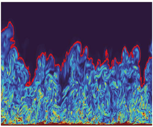
The instantaneous enstrophy contour plot and the instantaneous TNTI recognized by the enstrophy method and UMZ method are shown in figure 11. It can be seen that though these two TNTIs are similar, the TNTI identified by the UMZ method does not match well with the outer edge of the enstrophy field. The interface is so smooth that it can be considered as having some small-scale information erased from it. In contrast, the small wrinkle structures of the TNTI recognized by the enstrophy method match well with the outer edge of the enstrophy field, indicating that the enstrophy method effectively recognizes multiscale features on the TNTI, which is beneficial for subsequent analysis. The TNTI identified by the enstrophy method within the area between $Re_x=1.95 \times 10^6$–$2.41 \times 10^6$ has been used to investigate the properties of the TNTI.

Figure 11. Instantaneous enstrophy contour plot and instantaneous TNTI recognized by enstrophy method and UMZ method.

The geometric features of the interface are closely related to the entrainment, and the height of the TNTI is discussed in the paper. The mean value and r.m.s. value of the interface height at different streamwise positions are shown in figure 12. At the inlet of flat plate, the flow state is laminar, and the height of the interface $Y_{i}$ is equivalent to the thickness of the boundary layer. As the flow gradually develops into turbulence the $Y_{i}/\delta$ rapidly decreases and the normalized r.m.s. $\sigma _{i}/\delta$ gradually increases, indicating that the outer edge of the boundary layer is becoming more and more intermittent with the transition. In the turbulent region, $Y_{i}/\delta$ and $\sigma _{i}/\delta$ tend to stabilize at 0.85 and 0.15, respectively. The comparison between this result and the results of incompressible TBL in some previous works (Corrsin & Kistler Reference Corrsin and Kistler1995; Wu et al. Reference Wu, Wang, Cui and Pan2020) is shown in table 1. It can be seen that when the Mach number is 2.9, compressibility tends to increase the mean height of the interface. In this paper the mean height is increased by 3.7 %. The mechanism will be explored in § 4.

Figure 12. Streamwise variation of mean and r.m.s. interface height.

Table 1. Comparison of mean and r.m.s. height with previous works.

3.2. Interface thickness and fractal characteristics

The conditional average profiles of enstrophy are used in this article to obtain the interface thickness. An interface coordinate system is established to get conditional average profiles (Watanabe et al. Reference Watanabe, Zhang and Nagata2018). As shown in figure 13, the vertical axis of the interface coordinate is perpendicular to the interface. A small difference between the coordinate established in this article and figure 13 is that the vertical axis does not point to the non-turbulent region but points to the turbulent region. This means that when the vertical axis $y_I$ is positive, it is located inside the turbulent zone. Here $y_{I}$ ranges from $-95\eta$ to $95\eta$ and is discretized by 100 points. The flow at the height of $0.5\delta$ is used as the reference layer to calculate the Kolmogorov scale $\eta$. For the case where the coordinate passes through the interface multiple times, the area within 10 points away from the interface will be ignored, as shown by the dashed line in figure 13.

Figure 13. Establishment of interface coordinate axis (Watanabe et al. Reference Watanabe, Zhang and Nagata2018).

Figure 14 shows the conditional mean profile of enstrophy within the range $Re_x=1.28\times 10^6$–$1.46 \times 10^6$, where the black curve represents the enstrophy, and the red dashed line represents the derivative with respective to the interface coordinate $y_I$. The interface thickness $\delta _{i}$ is calculated based on the interval between the position where the derivative reaches 20 % of the peak value and the position where the interface coordinate $y_I$ is 0 (Zhang et al. Reference Zhang, Watanabe and Nagata2018b), as shown in the shaded part of the figure. The interface thickness is approximately 16.8$\eta$. This change in average thickness may be caused by the increase of $Ma$ and Reynolds number. The comparison of interface thickness with previous results by Zhang et al. (Reference Zhang, Watanabe and Nagata2018b, Reference Zhang, Watanabe and Nagata2023) is shown in figure 15. It has been found that as the $Re_\theta$ increases, the mean thickness of the TNTI remains almost unchanged within approximately $15.7\eta$ (Zhang et al. Reference Zhang, Watanabe and Nagata2023) while the increase of $Ma$ has a significant effect on the thickness (Zhang et al. Reference Zhang, Watanabe and Nagata2018b) with limited data. This shows that the compressibility may tend to increase the mean thickness of the interface. In this paper the thickness is increased by approximately 7.0 %. A potential mechanism related to compressibility will be explained in § 4, however, more data is needed to reveal it.

Figure 14. Conditioned mean profile of enstrophy field and its derivative with respective to interface coordinate $y_{I}$.

Figure 15. Comparison of interface thickness with the works by Zhang et al. (Reference Zhang, Watanabe and Nagata2018b, Reference Zhang, Watanabe and Nagata2023).

The fractal dimension is used to describe the fractal characteristics of the interface, and the box-counting method is used to analyse the interface in the range of $Re_{x}= 0$$-$$2.79\times 10^5,2.79\times 10^5$$-$$5.58\times 10^5,5.58\times 10^5$$-$$8.37 \times 10^5,8.37\times 10^5$$-$$1.12 \times 10^6$, $1.12 \times 10^6$$-$$1.40 \times 10^6,\, 1.40 \times 10^6$$-$$1.67 \times 10^6,\ 1.67 \times 10^6$$-$$1.95 \times 10^6,\ 1.95 \times 10^6$$-$$2.23 \times 10^6$. The box size range is $0.01\delta$$-\delta$. The corresponding relationship between $N_{b}$ and $r$ in the range of $Re_x=1.95\times 10^6$–$2.23 \times 10^6$ is shown in figure 16(a). The blue circle represents the number of boxes corresponding to different box sizes, and the red solid line represents the fitting result. The slope of the fitted line is approximately $-$1.18. According to (1.1), the fractal dimension $D$ is approximately 1.18 and $D_f$ is approximately 2.18, which is slightly smaller than the previous result of incompressible TBL with $D_f=2.3$ (de Silva et al. Reference de Silva, Philip, Chauhan, Meneveau and Marusic2013). This may be related to the small Reynolds number and Mach number of the flow, rather than the influence of compressibility. The comparison of fractal dimension results between the present work and some previous works is shown in figure 17, which indicates that the fractal dimensions are affected by the Reynolds number and $D_f$ may get closer to 2.3 at a higher Reynolds number (Zhang et al. Reference Zhang, Watanabe and Nagata2023) while the $Ma$-dependency of $D_f$ still lacks investigation. However, the fractal dimension in a compressible supersonic TBL with $Ma = 2.83$ and $Re_\theta = 9.14 \times 10^4$ has been investigated (Zhuang et al. Reference Zhuang, Tan, Huang, Liu and Zhang2018) and it was found that the $D_f$ is 2.31, which is consistent with the results of high Reynolds number. This may indicate that the Mach number has little effect on the fractal dimension, but further research is still needed to support it. Figure 16(b) shows the streamwise variation of the fractal dimension. It can be seen that the fractal dimension of the interface gradually increases, which indicates that with the development of the flow, the intermittency of the boundary layer increases, and the TNTI also becomes more distorted. In the turbulent region, the fractal dimension gradually approaches approximately 1.18 in this investigation. As the flow further develops, $D_f$ may increase further.

Figure 16. The fractal characteristic of TNTI. (a) Interface fractal dimension in the range of $Re_{x}=1.95\times 10^6$–$2.23 \times 10^6$. (b) The streamwise variation of fractal dimension.

Figure 17. Comparison of fractal dimension results between present work and previous works.

4.1. Enstrophy transport characteristics

The conditional mean profiles of the production term, viscous diffusion term and viscous dissipation term on both sides of the interface are shown in figure 18: the blue solid line represents the production term, the green dotted line represents the viscous diffusion term and the red dashed line represents the viscous dissipation term. These three terms are roughly of the same order of magnitude near the interface. The conditional mean profiles of the compressibility independent terms are basically consistent with those in the incompressible TBL (Watanabe et al. Reference Watanabe, Zhang and Nagata2018; Zhang et al. Reference Zhang, Watanabe and Nagata2018b; Long et al. Reference Long, Wang and Pan2022).

Figure 18. Conditional mean profiles of production, viscous diffusion and viscous dissipation.

The conditional mean profiles of $\varOmega _{I}$–$\varOmega _{VI}$ and $\mathrm {D}\varOmega /\mathrm {D}t$ are shown in figure 19, where the black dashed line represents the total enstrophy transportation. The production term, viscous dissipation term and viscous diffusion term have a large magnitude near the interface, indicating that these three terms play a dominant role in the entrainment. However, the dilatation term, baroclinic term and density gradient term caused by compressibility have a smaller order of magnitude, which is shown as a straight line near zero in the figure.

Figure 19. Conditional mean profiles of enstrophy transport components.

In order to further investigate the influence of compressibility on the enstrophy transportation, figure 20(a) compares the conditional mean profiles of the contribution of compressibility independent terms and the total enstrophy transportation. It can be spotted that the two are in good agreement in most areas, and $\mathrm {D}\varOmega /\mathrm {D}t$ has a certain change compared with the contribution of compressibility independent terms in the entire interface thickness. The changes near the interface are magnified in figure 20(a), which shows that ${\rm D}\varOmega /{\rm D}t$ is decreased due to the compressibility-related terms near the interface especially at the interface coordinate $y_I=1.9\eta$ (the red line). The proportion of compressibility-related terms in the total enstrophy transportation at different locations in the interface coordinate is shown in figure 20(b), which proves the conclusion above. The proportion gradually decreased from approximately 2 % outside the interface, began to decline rapidly at the interface coordinate 0 and then reached the minimum value of $-$13.4 % at $y_{I}=1.9\eta$. This suggests that compressibility tends to reduce the enstrophy of the turbulent fluids near the interface. After the minimum value, the proportion of the compressibility-related terms rapidly changes to a positive value with a maximum value of approximately 5.4 %, indicating that the compressibility tends to increase the enstrophy of the fluids far away from the interface. After exceeding the interface thickness the contribution of compressibility is stable at approximately $1\,\%$–$2\,\%$.

Figure 20. The influence of compressibility. (a) Comparison of total enstrophy transportation and the contribution of compressibility irrelevant items. The changes near the interface are magnified. (b) Proportion of compressibility-related terms plotted against different locations in the interface coordinate system.

To make sure that the evaluation is reliable, the convergence of the result is investigated in figure 21. As the number of samples increases, the minimum percentage and its position in the interface coordinate become stable, which is $-$13 % and $y_I=1.9\eta$, respectively. This shows that compressibility tends to transfer the enstrophy of turbulence near the interface to both directions vertical to the interface, which promotes the expansion of the turbulent region to the non-turbulent region. This is also the reason why the mean height and the mean thickness of the interface are larger than those of the incompressible TBL (Corrsin & Kistler Reference Corrsin and Kistler1995; Wu et al. Reference Wu, Wang, Cui and Pan2020) and compressible TBL with lower Mach number in the previous works (Zhang et al. Reference Zhang, Watanabe and Nagata2018b).

Figure 21. Convergence verification of compressibility effect. (a) The variation of minimum percentage plotted against the number of samples. (b) The position of the minimum percentage in the interface coordinate plotted against the number of samples.

4.2. Entrainment characteristics

From (4.8) and (4.3), the entrainment velocity of compressible flow can be calculated as follows:

(4.9)\begin{align} v_{n} &= \frac{-2\omega_{i}\omega_{j}\dfrac{\partial u_{i}}{\partial x_{j}}}{|\boldsymbol{\nabla} \varOmega|}+ \frac{2\varOmega \dfrac{\partial u_{j}}{\partial x_{j}}}{|\boldsymbol{\nabla} \varOmega|} - \frac{\dfrac{2\omega_{i}\epsilon_{ijk}}{\rho^2} \dfrac{\partial \rho}{\partial x_{j}} \dfrac{\partial p}{\partial x_{k}}}{|\boldsymbol{\nabla} \varOmega|} - \frac{\nu\dfrac{\partial^2 \varOmega}{\partial x_{j} \partial x_{j}}}{|\boldsymbol{\nabla} \varOmega|} \nonumber\\ &\quad +\frac{2\nu \dfrac{\partial \omega_{i}}{\partial x_{j}} \dfrac{\partial \omega_{i}}{\partial x_{j}}}{|\boldsymbol{\nabla} \varOmega|} + \frac{\dfrac{2\omega_{i}\epsilon_{ijk}}{\rho^2} \dfrac{\partial \rho}{\partial x_{j}} \dfrac{\partial \tau_{km}}{\partial x_{m}}}{|\boldsymbol{\nabla} \varOmega|}. \end{align}

The p.d.f. of the entrainment velocity calculated from (4.9) is shown in figure 22(a). The p.d.f. deviates from the standard Gaussian distribution and has a negative skewness, which indicates that the turbulent region has a trend of outward expansion. The result is in good agreement with the previous results of incompressible TBL (Wolf et al. Reference Wolf, Lüthi, Holzner, Krug, Kinzelbach and Tsinober2012; Mistry et al. Reference Mistry, Philip and Dawson2019; Long et al. Reference Long, Wang and Pan2022) and compressible TBL (Zhang et al. Reference Zhang, Watanabe and Nagata2018b). Figure 22(b) shows the p.d.f. of the contributions of different terms ($v_{nI}$–$v_{nVI}$, respectively) to the entrainment velocity, which is basically consistent with the previous result of the compressible flat TBL (Zhang et al. Reference Zhang, Watanabe and Nagata2018b). The production term and viscous diffusion term have a large negative skewness, with the values of $-$3.04 and $-$2.83, respectively, while the skewness of the viscous dissipation term is positive, approximately 3.39. The skewness of the dilatation term and the baroclinic term is 0.38 and 0.34, respectively, which is smaller than compressibility independent terms. This indicates that the compressibility independent terms play a key role in the entrainment. Though the contribution of the compressibility-related term is small, it cannot be ignored.

Figure 22. (a) Probability density function of entrainment velocity. (b) Probability density function of the contribution of different components to the entrainment velocity.

Further statistical analysis shows that the average contribution of $-v_{nI}$–$-v_{nVI}$ (negative sign ensures positive entrainment when the mean value is positive) to the entrainment normalized by Kolmogorov velocity is approximately 0.22, 0.10, 0.01, 8.96, $-$7.99 and 0.0001, respectively; and the entrainment velocity is approximately 1.30 normalized by the Kolmogorov velocity. It can be seen that the mean contribution of the compressibility independent terms is relatively large and plays a key role in the entrainment. The mean entrainment velocity is increased by 8.5 % due to the contribution of compressibility.

Based on the analysis of the p.d.f. and the mean value of entrainment velocity, it is shown that there may be a large deviation between instantaneous local entrainment velocity and its mean value. In order to explore the distribution law of instantaneous entrainment velocity, the relationship between local entrainment velocity and interface curvature is discussed according to the ideas of previous studies (Wolf et al. Reference Wolf, Lüthi, Holzner, Krug, Kinzelbach and Tsinober2012, Reference Wolf, Holzner, Lüthi, Krug, Kinzelbach and Tsinober2013; Jahanbakhshi & Madnia Reference Jahanbakhshi and Madnia2016; Mistry et al. Reference Mistry, Philip and Dawson2019). In a two-dimensional interface, the curvature can be calculated by (4.10) (Mistry et al. Reference Mistry, Philip and Dawson2019; Balamurugan et al. Reference Balamurugan, Rodda, Philip and Mandal2020), where $s$ represents the length travelled along the interface curve starting from the starting point. Here $x$ and $y$ are the point coordinates on the interface, respectively. The positive curvature means that looking from the turbulent region, the interface has a concave surface towards the turbulent region; negative curvature means that the interface protrudes towards the non-turbulent region, forming a convex surface:

(4.10)\begin{equation} \kappa = \frac{\dfrac{\mathrm{d}\kern0.7pt x}{\mathrm{d}s} \dfrac{\mathrm{d}^2 y}{\mathrm{d}s^2} - \dfrac{\mathrm{d}y}{\mathrm{d}s} \dfrac{\mathrm{d}^2 x}{\mathrm{d}s^2}}{\left[\left(\dfrac{\mathrm{d}\kern0.7pt x}{\mathrm{d}s}\right)^2 + \left(\dfrac{\mathrm{d}y}{\mathrm{d}s}\right)^2\right]^{{3}/{2}}} .\end{equation}

Figure 23(a–c) shows the joint p.d.f.s of the contribution of production term, viscous diffusion term and viscous dissipation term to the entrainment velocity and the local curvature of the interface. The red dotted line marks the ridge line of joint p.d.f., and the slope of the ridge line can be used to characterize the change of the contribution value with the local curvature. In figures 23(a) and 23(c), the ridge line is slightly tilted with a positive slope, indicating that as the local curvature of the interface increases, the contribution of the production term and viscous dissipation term to the entrainment decreases. In figure 23(b), the ridge line inclines more violently, and the slope is negative. This indicates that the contribution of the viscous diffusion term to the entrainment velocity has a significant increase with the increase of interface curvature. The total contribution of the compressibility independent terms composed of production term, viscous diffusion term and dissipation term to the entrainment velocity also shows a correlation with the interface curvature, as shown in figure 23(d).

Figure 23. Joint p.d.f.s of local curvature and (a) production term, (b) viscous diffusion, (c) viscous dissipation, (d) compressibility independent term.

For the terms related to compressibility, figure 24(a–c) shows the joint p.d.f.s of the contribution of (figure 24a) the dilatation term, (figure 24b) the baroclinic term, (figure 24c) the density gradient term and the local curvature of the interface. For these three terms, the ridge lines tend to be horizontal. This shows that the contribution of the compressibility-related terms to the entrainment velocity is basically independent of the local curvature of the interface. Figure 24(d) shows the joint density function of the entrainment velocity and local interface curvature. The ridge line is obviously inclined, and the slope is negative, indicating that the absolute value of the entrainment velocity is larger in the highly curved concave surface, while it is the opposite in the convex surface area. This suggests that the intense entrainment tends to occur near the highly curved concave surface of the interface (Wolf et al. Reference Wolf, Lüthi, Holzner, Krug, Kinzelbach and Tsinober2012; Jahanbakhshi & MadniaReference Jahanbakhshi and Madnia2016).

Figure 24. Joint p.d.f.s of local curvature and (a) the dilatation term, (b) the baroclinic term, (c) the density gradient term, (d) the entrainment velocity.

The influence of additional terms of enstrophy transport equation caused by compressibility on the interface entrainment is mainly analysed above, and the influence of compressibility on local entrainment mass flux will be further discussed in thefollowing.

The compressibility of fluids is generally reflected in the expansion or compression of local volume, which can be quantitatively described by the dilatation, also known as the velocity divergence $\boldsymbol {\nabla }\boldsymbol{\cdot } U$. The p.d.f. of the velocity divergence is shown in figure 25. The peak value of the p.d.f. is located in the expansion area, and the probability of the expansion area on the TNTI is slightly greater than the probability of the compression area. In this work, the proportion of the expansion area is approximately 53.4 % of the interface.

Figure 25. Probability density function of velocity divergence.

The local entrainment mass flux can be determined by (Jahanbakhshi & Madnia Reference Jahanbakhshi and Madnia2016)

(4.11)\begin{equation} m={-}\rho \cdot v_{n}, \end{equation}

and the negative sign is used to ensure that the mass flux is positive when the interface entrains.

The conditional mean profiles of the contribution of different terms in (4.8) to the entrainment mass flux conditioned on the divergence of the velocity are shown in figure 26, and the contribution of the production term slightly increases with the increase of velocity divergence. The dilatation term gradually decreases with the increase of velocity divergence. In the compression region, the dilatation term exhibits a positive effect, while in the expansion region the effect is negative. The viscous diffusion and dissipation term is relatively large in areas where the absolute value of divergence is not large. As the absolute value of divergence increases, the contribution of viscous diffusion and dissipation gradually decreases, indicating that the compression and expansion of the fluid have a certain hindrance effect on the viscosity at the interface. The baroclinic term and density gradient term are of small order of magnitude, and their effects on entrainment mass flux are not obvious. The hindrance effect of the compression and expansion of the fluids on the viscosity is not consistent in performance. For $-0.02<\boldsymbol {\nabla }\boldsymbol{\cdot } U<0$, as $\boldsymbol {\nabla }\boldsymbol{\cdot } U$ decreases, the contribution of viscous diffusion and dissipation to the entrainment flux gradually decreases. For $\boldsymbol {\nabla }\boldsymbol{\cdot } U<-0.02$, as the velocity divergence decreases, the contribution of viscosity to local entrainment flux remains basically unchanged. However, for $\boldsymbol {\nabla }\boldsymbol{\cdot } U>0.01$, as the velocity divergence increases, the contribution of viscosity gradually decreases and the absolute value of the slope gradually increases, indicating that the expansion has a more significant hindrance effect on the viscosity at the interface. The entrainment mass flux has a large positive value where the absolute value of divergence is small. With the increase of the absolute value of divergence, the hindrance effect reduces the contribution of viscosity to the entrainment flux, while the contribution of the dilatation term is opposite in the two regions. The superposition of the two makes the entrainment mass flux still positive in most of the compression regions and negative in the expansion regions. Therefore, interface entrainment is considered to mainly occur in areas with compression and slight expansion. The local entrainment mass flux is mainly dominated by the dilatation term, production term and viscosity terms, of which the dilatation term and production term have positive effects. The contribution of viscosity terms is positive only where the absolute value of divergence is small.

Figure 26. Local entrainment mass flux plotted against velocity divergence. Here $\bar {\theta }$ is the mean momentum thickness.

The mechanism of the hindrance effect of compressibility on viscous terms can be related to the behaviour of the dilatation term since it plays the biggest role in the part of compressible terms. The instantaneous contour plots of $\varOmega _{II}$ and $\lambda _{ci}$ have been shown in figure 27 to investigate the relationship between the dilatation term and local flow structures. It can be seen that the local maximum values of $\varOmega _{II}$ are strongly associated with the vortex structures. More detailed distribution of $\varOmega _{II}$ and the corresponding $\lambda _{ci}$ fields near the interface has been provided in figure 28. As the dilatation term can be calculated as $\varOmega _{II} = - 2 \varOmega ({\partial u_i}/{\partial x_i})$, the local maximum values should be strongly connected with the local maximum values of the enstrophy and $\lambda _{ci}$ fields, and the plus or minus signs of the values are determined by the local flow state of compression or expansion. In the expansion area, the local minimum values of $\varOmega _{II}$ appear while in the compression area the situation is the opposite. The expansion causes the enstrophy to diffuse outwards, making the interface develop from concave surface to convex surface and increasing the average height of the interface. The change in the geometry characteristic of the interface suppresses the viscous term, forming the hindrance effect. Some fluids may even pass through the interface forming detrainment, which corresponds to the results of $m_{II}$ in figure 26. In the compression area, the convergence of the fluids enhances the entrainment process and forms a highly concave surface at the interface, which is conducive to the effect of viscous terms.

Figure 27. The instantaneous contour plots of dilatation terms $\varOmega _{II}$ and $\lambda _{ci}$.

Figure 28. Local details of instantaneous contour plots of $\varOmega _{II}$ and $\lambda _{ci}$.

The local minimum and maximum values of $\varOmega _{II}$ within the interface thickness range have been selected and the conditional mean profiles have been shown in figure 29. It can be observed that though the distributions show different tendencies along the coordinate, a local minimum value exists near the outer edge of the interface at $y_{I} \approx 2.5 \eta$. This can be caused by the proportions of the expansion and compression area since the expansion area is larger than the compression area with a percentage of $53\,\%$–$54\,\%$, which leads to the decrease in the total enstrophy transportation $\mathrm {D}\varOmega /\mathrm {D}t$.

Figure 29. Conditional mean profiles of local minimum and maximum values of dilatation term.

A fact that needs to be elaborated on is that the conditional mean profiles of the dilatation term have a negative valley near the outer edge of the interface, which should have led to a negative contribution to the entrainment velocity. However, the dilatation term actually makes a positive contribution. This should be connected to the influence of the compressibility on the gradient of enstrophy $|\boldsymbol {\nabla } \varOmega |$. In the expansion area, the diffusion of enstrophy is enhanced, which increases the gradient of enstrophy $|\boldsymbol {\nabla } \varOmega |$. In the compression area, the diffusion of enstrophy is suppressed, and $|\boldsymbol {\nabla } \varOmega |$ also decreases. According to (4.3), the absolute values of the entrainment velocity contributed by the dilatation term in the compression region should be greater than the expansion area, which results in the conditional mean contribution to the entrainment velocity of the dilatation term remaining positive. The conditional mean profile of the $|\boldsymbol {\nabla } \varOmega |$ plotted against the dilatation term has been shown in figure 30. The symbol of the expansion pressure term represents the expansion and compression state of the fluid, with negative values indicating the expansion state and positive values indicating the compression state. It can be observed that in the case where the absolute values of the dilatation term are equal, $|\boldsymbol {\nabla } \varOmega |$ in the expansion area is greater than the compression area, which is consistent with the previous discussion. As the compressibility increases, the phenomenon may become more obvious. A lower $|\boldsymbol {\nabla } \varOmega |$ can also suppress the effect of viscous terms, that is why though compression is beneficial for the viscous terms, $m_{IV} + m_{V}$ is still negative in the compression area.

Figure 30. The conditional mean profile of the $|\boldsymbol {\nabla } \varOmega |$ plotted against the dilatation term.