


1. Introduction
Gas-particle two-phase flow appears in chemical, petroleum, environmental and other industries. Quantitative study of the system is of great importance in both basic scientific research and practical industrial production (Marchisio & Fox Reference Marchisio and Fox2013; Ceresiat, Kolehmainen & Ozel Reference Ceresiat, Kolehmainen and Ozel2021). Most granular flow systems include multiple types of solid particles with different material densities, diameters, shapes, etc., which is named as the polydisperse gas-particle flow. For the polydisperse system, it may become problematic to regard all kinds of solid particles as a single phase, especially as particle properties differ significantly from each other. For instance, the inter-phase heat conduction and the rate of chemical reaction highly depend on the solid particle's size. As a result, the effect from the particle size distribution (PSD) cannot be ignored (Zhong et al. Reference Zhong, Yu, Zhou, Xie and Zhang2016; Yan et al. Reference Yan, Dong, Zhou and Luo2023). Besides, the mixing and segregation of different types of solid particles are important issues that deserve much attention in the chemical and food industries, and thus the numerical method for the multi-disperse particulate flow should be employed (Fox & Vedula Reference Fox and Vedula2010). In addition, the interaction between different types of solid particles, which is usually modelled by the so-called solid-to-solid drag, plays a significant role in predicting the particles’ behaviours, indicating the necessity of accurately modelling the polydisperse system (Syamlal Reference Syamlal1987; Mathiesen et al. Reference Mathiesen, Solberg, Arastoopour and Hjertager1999). Therefore, developing an advanced computational fluid dynamics tool for polydisperse gas-particle flow is more challenging than its monodisperse counterparts due to the increased complexity in the multi-particle system (Zhang et al. Reference Zhang, Xu, Chang, Zhao, Wang and Ge2023).
Generally, two approaches, Eulerian–Eulerian (EE) approach and Eulerian–Lagrangian (EL) approach, are used for the study of gas-particle two-phase flow. In both approaches, the gas phase is described by the Navier–Stokes (NS) equations, i.e. the so-called Eulerian approach; while the treatment of the solid particle phase can be Eulerian or Lagrangian. In the EE approach, the particle phase is modelled as a continuum fluid, and the hydrodynamic solvers are used in the simulation (Gidaspow Reference Gidaspow1994; Saurel & Abgrall Reference Saurel and Abgrall1999; Lu & Gidaspow Reference Lu and Gidaspow2003). In the EL approach, all solid particles or parcels, standing for a group of solid particles with the same properties, are tracked individually by solving the Newtonian equation of particle motion. At the same time, the collisions between solid particles are modelled, such as these collision rules in the discrete element method (DEM) (Tsuji, Kawaguchi & Tanaka Reference Tsuji, Kawaguchi and Tanaka1993; Zhang et al. Reference Zhang, Zhao, Lu, Ge, Wang and Duan2017b) and in the multiphase particle-in-cell method (MP-PIC) (Snider Reference Snider2001, Reference Snider2007; Verma & Padding Reference Verma and Padding2020). In general, the EL approach works well in all flow regimes. Although the EE approach may not be able to accurately predict the particular flow when the Knudsen number (Kn) of the solid phase is large, it is still the dominant method in practical engineering applications due to the efficiency of the EE approach in comparison with the EL one (Zhong et al. Reference Zhong, Yu, Zhou, Xie and Zhang2016; Zhang et al. Reference Zhang, Xu, Chang, Zhao, Wang and Ge2023). However, the recent studies also show that at some points the EL approach may be more accurate and efficient than the finely resolved two-fluid EE model (Benyahia Reference Benyahia2022). In addition to the aforementioned methods, other commonly used numerical methods for granular flow include, but are not limited to, method of moment (Fan & Fox Reference Fan and Fox2008; Marchisio & Fox Reference Marchisio and Fox2013), direct simulation of Monte Carlo (He et al. Reference He, Zhao, Wang and Zheng2015), compressible multiphase particle-in-cell method (Tian et al. Reference Tian, Zeng, Meng, Chen, Guo and Xue2020) and hybrid EL method (Zhang et al. Reference Zhang, Wang, Lu, Liu, Wang and Zhao2017a), and many others.
For the solid particle evolution, the dynamics from the particle free transport with the interaction with the gas phase and inter-particle collisions should be modelled (Marchisio & Fox Reference Marchisio and Fox2013; Yang et al. Reference Yang, Wei, Shyy and Xu2023). For the polydisperse flow, the inter-particle collision includes the monodisperse and polydisperse types of particles. For the EL approach, such as DEM, the effect on the particle in the polydisperse case can be added straightforwardly in the simulation, since all solid particles’ transport will be tracked with the explicit inter-particle collision according to the collision law (Feng et al. Reference Feng, Xu, Zhang, Yu and Zulli2004; Zhang et al. Reference Zhang, Zhao, Lu, Ge, Wang and Duan2017b). However, the computational cost is high, especially at small Kn, due to the explicit tracking of tremendous amount of particles. For the EE approach, the multi-fluid strategy is one of the commonly adopted methods in the polydisperse flow study, where many sets of governing equations are employed to describe the disperse phases (Mathiesen et al. Reference Mathiesen, Solberg, Arastoopour and Hjertager1999; Lu & Gidaspow Reference Lu and Gidaspow2003). For example, in the study of hydrodynamic behaviours from the PSD, the particle phase is modelled in different discrete phases according to the particle size (Qin, Zhou & Wang Reference Qin, Zhou and Wang2019). In the multi-fluid model, the closure of one solid phase will involve the properties of other disperse phases. It becomes crucially important to develop valid numerical methods for polydisperse gas-particle flow (Zhao & Wang Reference Zhao and Wang2021). The determination of the solid-to-solid drag in the momentum exchange between different disperse phases has to be properly modelled (Syamlal Reference Syamlal1987; Mathiesen et al. Reference Mathiesen, Solberg, Arastoopour and Hjertager1999; Fan & Fox Reference Fan and Fox2008). Another approach is to use one set of governing equations for the whole solid phase, and additional modifications are added with the consideration of different particle sizes (Chen, Wang & Li Reference Chen, Wang and Li2013).
In addition, the gas–solid interaction also plays a significant role in monodisperse/polydisperse particular flow in both EE and EL approaches. In particular, the drag on a solid particle from the gas flow is of great importance to accurately predict the flow field of the gas-particle system (Li et al. Reference Li, Lan, Xu, Wang, Lu and Gao2009; Zhang et al. Reference Zhang, Zhao, Lu, Ge, Wang and Duan2017b). For example, different polydisperse drag models are compared to evaluate their performance in capturing the mixing and segregation of different dispersed solid flows (Zhang et al. Reference Zhang, Zhao, Lu, Ge, Wang and Duan2017b). Two methods are widely adopted to construct the drag model in the polydisperse system. Firstly, each disperse phase uses directly the drag model developed for monodisperse flow (Lu & Gidaspow Reference Lu and Gidaspow2003; Fan & Fox Reference Fan and Fox2008). Secondly, the total drag of the whole multi-disperse system is evaluated from either experiment or direct numerical simulation (DNS) and is distributed to individual disperse phases according to the interaction rule (Cello, Di Renzo & Di Maio Reference Cello, Di Renzo and Di Maio2010; Rong, Dong & Yu Reference Rong, Dong and Yu2014). It is worth mentioning that the mesoscale flow structures in the gas–solid system have a significant effect on the modelling of phase interaction. Particularly, the energy-minimization multiscale (EMMS) theory has been systematically developed for gas-particle flow (Li & Kwauk Reference Li and Kwauk1994; Yang et al. Reference Yang, Wang, Ge and Li2003; Wang & Li Reference Wang and Li2007). Recently, the EMMS has been developed and employed in the polydisperse particular flow system, with a preferred hydrodynamic performance in the EE approach (Qin et al. Reference Qin, Zhou and Wang2019). Besides, the filtered subgrid model is another important mesoscale method for both monodisperse and polydisperse gas-particle two-phase flows (Zhu et al. Reference Zhu, Ouyang, Lei and Luo2021; Lei, Zhu & Luo Reference Lei, Zhu and Luo2023). For example, the material property-dependent drag model presents satisfactory results in comparison with the experiment measurements (Zhu et al. Reference Zhu, Liu, Tang and Luo2019a).
The unified gas-kinetic wave–particle (UGKWP) method is able to simulate the equilibrium and non-equilibrium transports in different regimes under a unified framework. The multiscale gas-kinetic scheme (GKS)-UGKWP method for gas-particle two-phase flow is a regime-adaptive method to recover the EE and EL approaches in the limiting conditions (Yang et al. Reference Yang, Liu, Ji, Shyy and Xu2022b; Yang, Shyy & Xu Reference Yang, Shyy and Xu2022c; Yang et al. Reference Yang, Wei, Shyy and Xu2023). The UGKWP is an extension of the unified gas-kinetic scheme (UGKS). The UGKS models the flow physics directly on the scales of cell size and time step (Xu & Huang Reference Xu and Huang2010; Xu Reference Xu2021). The method was initially developed for rarefied flow and further extended to radiation transfer, plasma, particular flow, etc. (Sun, Jiang & Xu Reference Sun, Jiang and Xu2015; Liu & Xu Reference Liu and Xu2017; Liu, Wang & Xu Reference Liu, Wang and Xu2019). Both UGKS and UGKWP update macroscopic flow variables. However, different from the UGKS method with the update of the gas distribution function with the discretized particle velocity space in a deterministic way, the UGKWP method decomposes the distribution function into analytical wave and statistical particle, where the weights for the wave and particle depend on the local cell's Knudsen number (Kn), such as  $(1-\exp (-1/\text {Kn}))$ for the wave component and
  $\exp (-1/\text {Kn})$ for the particle component. Due to the absence of a discretized particle velocity space, the UGKWP method increases its computational efficiency greatly in high-speed and high-temperature flow simulations, especially for flow simulation close to the equilibrium (Zhu et al. Reference Zhu, Liu, Zhong and Xu2019b; Liu, Zhu & Xu Reference Liu, Zhu and Xu2020). In the continuum flow regime, UGKWP gets back to the GKS (Xu Reference Xu2001, Reference Xu2021; Yang et al. Reference Yang, Ji, Shyy and Xu2022a), which is the kinetic theory-based second-order NS solver. The GKS is used directly to compute the gas phase in the current gas–solid particle system. Due to the Kn-dependent wave–particle decomposition, UGKWP is suitable for the simulation of particle flow. In the high particle collision regime with a small Kn, no particles will be sampled in UKGWP, and thus a hydrodynamic formulation will emerge for the evolution of the solid particle phase. The whole GKS-UGKWP will recover the EE approach automatically. On the contrary, when Kn is large, such as the collisionless regime for the solid particle phase, the evolution of the solid phase will be determined by tracking the discrete particles, and the GKS-UGKWP automatically gets back to the EL approach. At an intermediate Kn, both hydrodynamic wave and microscopic discrete particles will be updated in UGKWP for capturing the local non-equilibrium particle flow. In this paper, for the first time, the GKS-UGKWP is constructed to solve polydisperse gas-particle flow with multiple disperse particle phases, where particle's transport in the gas flow and particle collisions between same-type and different-type particles will be incorporated into the scheme.
This paper is organized as follows. Section 2 introduces the governing equations for the particle phase and the UGKWP method. Section 3 presents the governing equations for the gas phase and GKS method. Section 4 shows the numerical examples and the engineering applications with experimental measurements. The last section is the conclusion.
2. Unified gas-kinetic wave–particle method for disperse solid particle phase
2.1. Governing equation for disperse phase
The evolution of disperse phase is governed by the kinetic equation
 \begin{equation} \frac{\partial f_{k}}{\partial t} + \boldsymbol{\nabla}_{\boldsymbol{x}} \boldsymbol{\cdot} (\boldsymbol{u}f_{k}) + \boldsymbol{\nabla}_{\boldsymbol{u}} \boldsymbol{\cdot} (\boldsymbol{a}f_{k}) = \frac{g_{k}-f_{k}}{\tau_{k}} + \sum_{i=1,i\neq k}^{N} \frac{g_{ik}-f_{k}}{\tau_{ik}}, \end{equation}
where  $f_{k}$ is the distribution function of the
  $k$th disperse phase,
  $\boldsymbol {u}$ is the particle velocity,
  $\boldsymbol {a}$ is the particle acceleration caused by the external force,
  $\boldsymbol {\nabla }_{\boldsymbol {x}}$ is the divergence operator with respect to space,
  $\boldsymbol {\nabla }_{\boldsymbol {u}}$ is the divergence operator with respect to velocity,
  $\tau _k$ is the relaxation time for the
  $k$th disperse phase and
  $g_{k}$ is the associated equilibrium distribution, which can be written as
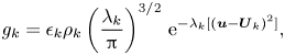 \begin{equation} g_{k}=\epsilon_k\rho_k\left(\frac{\lambda_k}{\rm \pi}\right)^{{3}/{2}}\,{\rm e}^{-\lambda_k [(\boldsymbol{u}-\boldsymbol{U}_k)^2]}, \end{equation}
where  $\epsilon _k$ is the volume fraction of the
  $k$th disperse phase,
  $\rho _k$ is the material density of the
  $k$th disperse phase,
  $\lambda _k$ is the variable relevant to the granular temperature
  $\theta _k$ with
  $\lambda _k = 1/(2\theta _k)$ and
  $\boldsymbol {U}_k$ is the macroscopic velocity of the
  $k$th disperse phase. The second term at the right-hand side
  $(g_{ik}-f_{k})/{\tau _{ik}}$ stands for the cross-species collision, where
  $N$ is the number of the solid disperse phase,
  $\tau _{ik}$ is the auxiliary collision time and
  $g_{ik}$ is the auxiliary equilibrium distribution
 \begin{equation} g_{ik}=\epsilon_k\rho_k\left(\frac{\lambda_k}{\rm \pi}\right)^{{3}/{2}}\,{\rm e}^{-\lambda_k [(\boldsymbol{u}-\boldsymbol{U}_{ik})^2]}, \end{equation}
and note that the mass conservation for the cross-species collision can be satisfied automatically with the above  $g_{ik}$.
The particle acceleration  $\boldsymbol {a}$ is determined by the external forces, such as the drag force
  $\boldsymbol {D}$, the buoyancy force
  $\boldsymbol {F}_b$ and gravity
  $m_k\boldsymbol {G}$, etc. Particularly,
  $\boldsymbol {D}$ and
  $\boldsymbol {F}_b$ are inter-phase forces, standing for the force applied on the solid particles by the gas flow. The general form of drag force can be evaluated by the drag force model
 \begin{equation} \boldsymbol{D} =\frac{m_k}{\tau_{st}}(\boldsymbol{U}_g-\boldsymbol{u}). \end{equation}
In the numerical simulation, the  $\tau _{st}$ in (2.4) will be closed by the drag model chosen for the solid phase, which will be introduced in detail later. Besides, another interactive force considered is the buoyancy force, which can be modelled as
 \begin{equation} \boldsymbol{F}_b ={-}\frac{m_k}{\rho_{k}} \boldsymbol{\nabla}_{\boldsymbol{x}} p_g, \end{equation}
where  $p_g$ is the pressure of the gas phase.
2.2. Unified gas-kinetic wave–particle method
In this subsection, the UGKWP for the evolution of disperse phase is introduced. Generally, the splitting operator is used to solve (2.1) through the following procedures within a numerical time step of the solid phase  $\Delta t_s$:
 $$\begin{gather} \mathcal{L}_{d1} :\enspace \frac{\partial f_{k}}{\partial t} + \boldsymbol{\nabla}_{\boldsymbol{x}} \boldsymbol{\cdot} (\boldsymbol{u}f_{k}) = \frac{g_{k}-f_{k}}{\tau_{k}}, \end{gather}$$
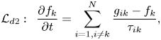 $$\begin{gather}\mathcal{L}_{d2} :\enspace \frac{\partial f_{k}}{\partial t} = \sum_{i=1,i\neq k}^{N} \frac{g_{ik}-f_{k}}{\tau_{ik}}, \end{gather}$$
 $$\begin{gather}\mathcal{L}_{d3} :\enspace \frac{\partial f_{k}}{\partial t} + \boldsymbol{\nabla}_{\boldsymbol{u}} \boldsymbol{\cdot} (\boldsymbol{a}f_{k}) = 0. \end{gather}$$
For brevity, the variables updated by  $\mathcal {L}_{d1}$,
  $\mathcal {L}_{d2}$ and
  $\mathcal {L}_{d3}$ are denoted as
 \begin{equation} \mathcal{L}_{d1}:\boldsymbol{W}^{n}\to\boldsymbol{W}^{*},\quad \mathcal{L}_{d2}:\boldsymbol{W}^{*}\to\boldsymbol{W}^{**}, \quad \mathcal{L}_{d3}:\boldsymbol{W}^{**}\to\boldsymbol{W}^{n+1}. \end{equation}
 Firstly, we focus on the part  $\mathcal {L}_{d1}:\boldsymbol {W}^{n}\to \boldsymbol {W}^{*}$. The disperse phase kinetic equation without external force and cross-species collisions of solid particles is
 \begin{equation} \frac{\partial f_{k}}{\partial t} + \boldsymbol{\nabla}_{\boldsymbol{x}} \boldsymbol{\cdot} (\boldsymbol{u}f_{k}) = \frac{g_{k}-f_{k}}{\tau_{k}}. \end{equation}
For brevity, the subscript  $k$ will be neglected in this subsection. The integral solution of the kinetic equation can be written as
 \begin{equation} f(\boldsymbol{x},t,\boldsymbol{u})=\frac{1}{\tau}\int_0^t g(\boldsymbol{x}',t',\boldsymbol{u} ) \,{\rm e}^{-(t-t')/\tau}\,\text{d}t'\\ +{\rm e}^{{-}t/\tau}f_0(\boldsymbol{x}-\boldsymbol{u}t, \boldsymbol{u}), \end{equation}
where  $\boldsymbol {x}'=\boldsymbol {x}+\boldsymbol {u}(t'-t)$ is the trajectory of the particle,
  $f_0$ is the initial distribution function at time
  $t=0$ and
  $g$ is the corresponding equilibrium state. In UGKWP, both macroscopic conservative variables and microscopic distribution function will be updated under a finite volume framework. The cell-averaged macroscopic variables
  $\boldsymbol {W}_i$ of cell
  $i$ are updated by the conservation law
 \begin{equation} \boldsymbol{W}_i^{*} = \boldsymbol{W}_i^n - \frac{1}{\varOmega_i} \sum_{S_{ij}\in \partial \varOmega_i}\boldsymbol{F}_{ij}S_{ij} + \boldsymbol{S}_{i} \Delta t, \end{equation}
where  $\boldsymbol {W}_i=(\epsilon _i\rho _i, \epsilon _i\rho _i \boldsymbol {U}_i, \epsilon _i\rho _i E_i)$ are the cell-averaged macroscopic variables defined as
 \begin{equation} \boldsymbol{W}_i = \frac{1}{\varOmega_{i}}\int_{\varOmega_{i}} \boldsymbol{W}(\boldsymbol{x}) \,\text{d}\varOmega, \end{equation}
where  $\epsilon _{i}\rho _iE_i = \frac {1}{2}\epsilon _{i}\rho _i \boldsymbol {U}_i^2 + \frac {3}{2}\epsilon _{i}\rho _i\theta _i$,
  $\varOmega _i$ is the volume of cell
  $i$,
$i$,  $\partial \varOmega _i$ denotes the set of cell interfaces of cell
  $i$,
$i$,  $S_{ij}$ is the area of the
  $j$th interface of cell
  $i$ and
  $\boldsymbol {F}_{ij}$ denotes the fluxes for
  $\boldsymbol {W}_i$ passing through the interface
  $S_{ij}$. The flux
  $\boldsymbol {F}_{ij}$ in one step
  $\Delta t$ can be calculated by
 \begin{equation} \boldsymbol{F}_{ij}=\int_{0}^{\Delta t} \int \boldsymbol{u}\boldsymbol{\cdot}\boldsymbol{n}_{ij} f_{ij}(\boldsymbol{x},t,\boldsymbol{u}) \boldsymbol{\psi}\, \text{d}\boldsymbol{u}\,\text{d}t, \end{equation}
where  $\boldsymbol {n}_{ij}$ is the unit normal vector of interface
  $S_{ij}$,
  $f_{ij}(t)$ is the distribution function on the interface
  $S_{ij}$ and
  $\boldsymbol {\psi }=(1,\boldsymbol {u},\frac {1}{2}\boldsymbol {u}^2)^{\rm T}$. Here
 \begin{equation} \boldsymbol{S}_{i} = \left[0,\textbf{0},-\frac{Q_{i,loss}}{\tau_k}\right]^{\rm T}, \end{equation}
stands for the lost energy due to the inelastic collision of solid particles
 \begin{equation} Q_{i,loss} = (1-{\rm e}^2)\tfrac{3}{2}\epsilon_{i} \rho_{i} \theta_i, \end{equation}
where  $e\in [0,1]$ is the restitution coefficient for the determination of the percentage of the lost energy in the inelastic collision, and
  $e$ has a value of 0.8, unless given specifically in this paper.
Substituting the time-dependent distribution function (2.11) into (2.14), the fluxes can be rewritten as
 \begin{align} \boldsymbol{F}_{ij} &=\int_{0}^{\Delta t} \int \boldsymbol{u}\boldsymbol{\cdot}\boldsymbol{n}_{ij} f_{ij}(\boldsymbol{x},t,\boldsymbol{u}) \boldsymbol{\psi} \,\text{d}\boldsymbol{u}\,\text{d}t\nonumber\\ &=\int_{0}^{\Delta t} \int\boldsymbol{u}\boldsymbol{\cdot}\boldsymbol{n}_{ij} \left[ \frac{1}{\tau}\int_0^t g(\boldsymbol{x}',t',\boldsymbol{u})\,{\rm e}^{-(t-t')/\tau}\,\text{d}t' \right] \boldsymbol{\psi} \,\text{d}\boldsymbol{u}\,\text{d}t\nonumber\\ &\quad +\int_{0}^{\Delta t} \int\boldsymbol{u}\boldsymbol{\cdot}\boldsymbol{n}_{ij} [ {\rm e}^{{-}t/\tau}f_0(\boldsymbol{x}-\boldsymbol{u}t,\boldsymbol{u})] \boldsymbol{\psi} \,\text{d}\boldsymbol{u}\,\text{d}t\nonumber\\ &\overset{def}{=}\boldsymbol{F}^{eq}_{ij} + \boldsymbol{F}^{fr}_{ij}. \end{align}
 The procedure for obtaining the local equilibrium state  $g_0$ at the cell interface and the construction of
  $g(t)$ are the same as that in GKS. For a second-order accuracy, the equilibrium state
  $g$ around the cell interface is written as
 \begin{equation} g(\boldsymbol{x}',t',\boldsymbol{u})=g_0(\boldsymbol{x},\boldsymbol{u}) (1 + \bar{\boldsymbol{a}} \boldsymbol{\cdot} \boldsymbol{u}(t'-t) + \bar{A}t'), \end{equation}
where  $\bar {\boldsymbol {a}}=[\overline {a_1}, \overline {a_2}, \overline {a_3}]^{\rm T}$,
  $\overline {a_i}=({\partial g}/{\partial x_i})/g$,
  $i=1,2,3$,
  $\bar {A}=({\partial g}/{\partial t})/g$ and
  $g_0$ is the local equilibrium on the interface. Specifically, the coefficients of spatial derivatives
  $\overline {a_i}$ can be obtained from the corresponding derivatives of the macroscopic variables
 \begin{equation} \langle \overline{a_i}\rangle=\partial \boldsymbol{W}_0/\partial x_i, \end{equation}
where  $i=1,2,3$, and
  $\langle \cdots \rangle$ means the moments of the Maxwellian distribution functions
 \begin{equation} \langle\cdots\rangle=\int \boldsymbol{\psi}(\cdots)g\,\text{d}\boldsymbol{u}. \end{equation}
The coefficients of temporal derivative  $\bar {A}$ can be determined by the compatibility condition
 \begin{equation} \langle \bar{\boldsymbol{a}} \boldsymbol{\cdot} \boldsymbol{u}+\bar{A} \rangle = \textbf{0}. \end{equation}
Now, all the coefficients in the equilibrium state  $g(\boldsymbol {x}',t',\boldsymbol {u})$ have been determined, and its integration becomes
 \begin{align} &f^{eq}(\boldsymbol{x},t,\boldsymbol{u}) \overset{def}{=} \frac{1}{\tau} \int_0^t g(\boldsymbol{x}',t',\boldsymbol{u})\,{\rm e}^{-(t-t')/\tau}\,\text{d}t' \nonumber\\ &\quad = c_1 g_0(\boldsymbol{x},\boldsymbol{u}) + c_2 \bar{\boldsymbol{a}} \boldsymbol{\cdot} \boldsymbol{u} g_0(\boldsymbol{x},\boldsymbol{u}) + c_3 A g_0(\boldsymbol{x},\boldsymbol{u}), \end{align}
with coefficients
 \begin{equation} \left.\begin{array}{c@{}}
c_1 = 1-{\rm e}^{{-}t/\tau}, \\ c_2 = (t+\tau)\,{\rm
e}^{{-}t/\tau}-\tau, \\ c_3 = t-\tau+\tau \,{\rm
e}^{{-}t/\tau}. \end{array}\right\}
\end{equation}
\begin{equation} \left.\begin{array}{c@{}}
c_1 = 1-{\rm e}^{{-}t/\tau}, \\ c_2 = (t+\tau)\,{\rm
e}^{{-}t/\tau}-\tau, \\ c_3 = t-\tau+\tau \,{\rm
e}^{{-}t/\tau}. \end{array}\right\}
\end{equation}
So, the flux from the equilibrium state  $\boldsymbol {F}^{eq}_{ij}$ is given by
 \begin{equation} \boldsymbol{F}^{eq}_{ij} =\int_{0}^{\Delta t} \int \boldsymbol{u}\boldsymbol{\cdot}\boldsymbol{n}_{ij} f_{ij}^{eq}(\boldsymbol{x},t,\boldsymbol{u})\boldsymbol{\psi}\,\text{d}\boldsymbol{u}\,\text{d}t. \end{equation}
 Besides, the flux contribution from the particle's free transport is calculated by tracking the particles sampled from  $f_0$. Therefore, the updating of the cell-averaged macroscopic variables can be written as
 \begin{equation} \boldsymbol{W}_i^{*} = \boldsymbol{W}_i^n - \frac{1}{\varOmega_i} \sum_{S_{ij}\in \partial \varOmega_i}\boldsymbol{F}^{eq}_{ij}S_{ij} + \frac{\boldsymbol{w}_{i}^{fr}}{\varOmega_{i}} + \boldsymbol{S}_{i} \Delta t, \end{equation}
where  $\boldsymbol {w}^{fr}_i$ is the net free streaming flow of cell
  $i$, obtained by counting the sampled particle, and it stands for the flux contribution of the free streaming of particles.
The evolution of the particle distribution can be written as
 \begin{equation} f(\boldsymbol{x},t,\boldsymbol{u}) =(1-{\rm e}^{{-}t/\tau})g^{+}(\boldsymbol{x},t,\boldsymbol{u}) +{\rm e}^{{-}t/\tau}f_0(\boldsymbol{x}-\boldsymbol{u}t,\boldsymbol{u}), \end{equation}
where  $g^{+}$ is named as the hydrodynamic distribution function with the analytical formulation. The initial distribution function
  $f_0$ has a probability of
  $\textrm {e}^{-t/\tau }$ to free transport and
  $(1-\textrm {e}^{-t/\tau })$ to collision with other particles. The post-collision particle satisfies the distribution
  $g^+(\boldsymbol {x},\boldsymbol {u},t)$. The free transport time before the first collision with other particles is denoted as
  $t_c$, and then the cumulative distribution function of
  $t_c$ is
 \begin{equation} F(t_c < t) = 1 - {\rm e}^{{-}t/ \tau}, \end{equation}
and therefore  $t_c$ can be sampled as
  $t_c=-\tau \ln (\eta )$, where
  $\eta$ is a random number generated from a uniform distribution
  $U(0,1)$. Then, the free streaming time
  $t_f$ for each particle is determined separately by
 \begin{equation} t_f = \min [-\tau\ln (\eta), \Delta t], \end{equation}
where  $\Delta t$ is the time step. Therefore, within one time step, all particles can be divided into two groups: the collisionless particle and the collisional particle, and they are determined by the relation between time step
  $\Delta t$ and free streaming time
  $t_f$. Specifically, if
  $t_f=\Delta t$, this particle is collisionless, and its trajectory is fully tracked in the whole time step. On the contrary, if
  $t_f<\Delta t$, this particle is a collisional one, and its trajectory is tracked until
  $t_f$. The collisional particle will be eliminated at
  $t_f$ in the simulation and the associated mass, momentum and energy carried by this particle are merged into the macroscopic quantities in the relevant cell by counting its contribution through the fluxes across the cell interfaces. More specifically, the particle trajectory in the free streaming process within time interval
  $t\in [0, t_f]$ is tracked by
 \begin{equation} \boldsymbol{x}^{*} = \boldsymbol{x}^n + \boldsymbol{u}^n t_f. \end{equation}
The term  $\boldsymbol {w}_{i}^{fr}$ can be calculated by counting the particles passing through the interfaces of cell
  $i$
$i$
 \begin{equation} \boldsymbol{w}_{i}^{fr} = \sum_{k\in P(\partial \varOmega_{i}^{+})} \boldsymbol{\phi}_k - \sum_{k\in P(\partial \varOmega_{i}^{-})} \boldsymbol{\phi}_k, \end{equation}
where  $P(\partial \varOmega _{i}^{+})$ is the particle set moving into cell
  $i$ within one time step,
  $P(\partial \varOmega _{i}^{-})$ is the particle set moving out of cell
  $i$,
$i$,  $k$ is the particle index in the specific set and
  $\boldsymbol {\phi }_k=[m_{k}, m_{k}\boldsymbol {u}_k, \frac {1}{2}m_{k}(\boldsymbol {u}^2_k)]^\textrm {T}$ is the mass, momentum and energy carried by particle
  $k$. Therefore,
  $\boldsymbol {w}_{i}^{fr}/\varOmega _{i}$ is the net conservative quantity caused by the free streaming of the tracked particles. Now, all the terms in (2.25) have been determined and the macroscopic variables
  $\boldsymbol {W}_i$ can be updated.
All particles have been traced up to time  $t_f$. The collisionless particle with
  $t_f=\Delta t$ will survive at the end of the time step; while the collisional particle with
  $t_f<\Delta t$ will be deleted after its first collision and it is assumed to go to the equilibrium state in that cell. Therefore, the hydrodynamic macroscopic variables of the collisional particles in cell
  $i$ at the end of each time step can be directly obtained by
 \begin{equation} \boldsymbol{W}^h_i = \boldsymbol{W}^{*}_i - \boldsymbol{W}^p_i, \end{equation}
and  $\boldsymbol {W}^p_i$ are the mass, momentum and energy of remaining collisionless particles in the cell. Here, the macroscopic variables
  $\boldsymbol {W}^h_i$ account for all eliminated collisional particles, which can be re-sampled from
  $\boldsymbol {W}^h_i$ based on the Maxwellian distribution at the beginning of the next time step. Now, the updates of both macroscopic variables and the microscopic particles have been presented. The above method is the so-called unified gas-kinetic particle (UGKP) method.
The above UGKP can be further developed to get an optimized UGKWP method in terms of efficiency and memory reduction. In the UGKP method, all particles are divided into collisionless and collisional particles in each time step. The collisional particles are deleted after the first collision and re-sampled from  $\boldsymbol {W}^h_i$ at the beginning of the next time step. However, only the collisionless portion of the re-sampled particles can survive in the next time step, and all re-sampled collisional ones will be deleted again. Fortunately, the transport fluxes from these collisional particles can be evaluated analytically without using particles. Therefore, we do not need to re-sample these collisional particles from
  $\boldsymbol {W}^h_i$ at all. According to the cumulative distribution (2.27), the proportion of collisionless particles is
  $\exp {(-\Delta t/\tau )}$, and therefore, in UGKWP, only the collisionless particles from the hydrodynamic variables
  $\boldsymbol {W}^{h}_i$ in cell
  $i$ will be re-sampled with the total mass, momentum and energy
 \begin{equation} \boldsymbol{W}^{hp}_i = {\rm e}^{-\Delta t/\tau} \boldsymbol{W}^{h}_i. \end{equation}
Then, the free transport time of all these re-sampled particles will be given by  $t_f=\Delta t$ in UGKWP. The fluxes
  $\boldsymbol {F}^{fr,wave}$ from these un-sampled collisional particles from
  $(1- \exp {(-\Delta t/\tau )} )\boldsymbol {W}^{h}_i$ can be evaluated analytically (Zhu et al. Reference Zhu, Liu, Zhong and Xu2019b; Liu et al. Reference Liu, Zhu and Xu2020). Now, the same as UGKP, in UGKWP, the net flux
  $\boldsymbol {w}_{i}^{fr,p}$ by the free streaming of the particles, which include remaining particles from the previous time step and re-sampled collisionless ones, can be calculated by
 \begin{equation} \boldsymbol{w}_{i}^{fr,p} = \sum_{k\in P(\partial \varOmega_{i}^{+})} \boldsymbol{\phi}_k - \sum_{k\in P(\partial \varOmega_{i}^{-})} \boldsymbol{\phi}_k. \end{equation}
So, the macroscopic flow variables in UGKWP are updated by
 \begin{equation} \boldsymbol{W}_i^{*} = \boldsymbol{W}_i^n - \frac{1}{\varOmega_i} \sum_{S_{ij}\in \partial \varOmega_i}\boldsymbol{F}^{eq}_{ij}S_{ij} - \frac{1}{\varOmega_i} \sum_{S_{ij}\in \partial \varOmega_i}\boldsymbol{F}^{fr,wave}_{ij}S_{ij} + \frac{\boldsymbol{w}_{i}^{fr,p}}{\varOmega_{i}} + \boldsymbol{S}_{i} \Delta t, \end{equation}
where  $\boldsymbol {F}^{fr,wave}_{ij}$ is the flux function from the un-sampled collisional particles (Zhu et al. Reference Zhu, Liu, Zhong and Xu2019b; Liu et al. Reference Liu, Zhu and Xu2020)
 \begin{align} \boldsymbol{F}^{fr,wave}_{ij} &=\boldsymbol{F}^{fr,UGKS}_{ij}(\boldsymbol{W}^h_i) - \boldsymbol{F}^{fr,DVM}_{ij}(\boldsymbol{W}^{hp}_i)\nonumber\\ &=\int_{0}^{\Delta t} \int \boldsymbol{u} \boldsymbol{\cdot} \boldsymbol{n}_{ij} [ {\rm e}^{{-}t/\tau}f_0(\boldsymbol{x}-\boldsymbol{u}t,\boldsymbol{u})] \boldsymbol{\psi} \,\text{d}\boldsymbol{u}\,\text{d}t\nonumber\\ &\quad -{\rm e}^{-\Delta t/\tau}\int_{0}^{\Delta t} \int \boldsymbol{u} \boldsymbol{\cdot} \boldsymbol{n}_{ij} [g_0^h(\boldsymbol{x},\boldsymbol{u}) - t\boldsymbol{u} \boldsymbol{\cdot} g_{\boldsymbol{x}}^h(\boldsymbol{x},\boldsymbol{u})] \boldsymbol{\psi}\,\text{d}\boldsymbol{u}\,\text{d}t\nonumber\\ &=\int \boldsymbol{u} \boldsymbol{\cdot} \boldsymbol{n}_{ij} \left[ (q_4 - \Delta t \,{\rm e}^{-\Delta t/\tau}) g_0^h (\boldsymbol{x},\boldsymbol{u}) + \left(q_5 + \frac{\Delta t^2}{2}\,{\rm e}^{-\Delta t/\tau}\right) \boldsymbol{u} \boldsymbol{\cdot} g_{\boldsymbol{x}}^h(\boldsymbol{x},\boldsymbol{u}) \right]\boldsymbol{\psi}\,\text{d}\boldsymbol{u}, \end{align}
with
 $$\begin{gather} q_4=\tau(1-{\rm e}^{-\Delta t/\tau}), \end{gather}$$
 $$\begin{gather}q_5=\tau\Delta t\,{\rm e}^{-\Delta t/\tau} - \tau^2(1-{\rm e}^{-\Delta t/\tau}). \end{gather}$$
 In the second part  $\mathcal {L}_{d2}$,
  $\boldsymbol {W}^{*}\to \boldsymbol {W}^{**}$ models the effect of cross-species collision between solid particles in different disperse phases. Taking the
  $k$th disperse phase for example, its collision with other disperse phases can be evaluated by
 \begin{equation} \frac{\partial f_{k}}{\partial t} = \sum_{i=1,i\neq k}^{N} \frac{g_{ik}-f_{k}}{\tau_{ik}}. \end{equation}
Obviously,  $\epsilon _{k}^{**}=\epsilon _k^{*}$ with the above formula of
  $g_{ik}$. Taking moment
  $\boldsymbol {\psi }=\boldsymbol {u}$ in the Euler regime with
  $f_k = g_k + {O}(\tau _{k})$, we can obtain
 \begin{equation} \frac{\partial ( \epsilon_{k}\rho_k\boldsymbol{U}_k )}{\partial t} = \sum_{i=1,i\neq k}^{N} \frac{\epsilon_k\rho_k(\boldsymbol{U}_{ik}-\boldsymbol{U}_k)}{\tau_{ik}}. \end{equation}
In this paper, the auxiliary velocity between the  $i$th and
  $k$th disperse phase,
  $\boldsymbol {U}_{ik}$, is assumed as
 \begin{equation} \boldsymbol{U}_{ik} = \frac{\epsilon_i \rho_i \boldsymbol{U}_i + \epsilon_k \rho_k \boldsymbol{U}_k}{\epsilon_i \rho_i + \epsilon_k \rho_k}. \end{equation}
Now, we need to determine  $\tau _{ik}$, i.e. the collision time between the
  $i$th and
  $k$th disperse phase. Generally, the commonly employed parameter in the polydisperse particular flow is
  $\beta _{ik}$, which is named the so-called inter-solid drag model and has the following relationship with
  $\tau _{ik}$:
 \begin{equation} \frac{\epsilon_k\rho_k(\boldsymbol{U}_{ik}-\boldsymbol{U}_k)}{\tau_{ik}} = \beta_{ik}(\boldsymbol{U}_{i}-\boldsymbol{U}_{k}). \end{equation}
Substituting (2.40) into (2.41), the expression of  $\tau _{ik}$ can be explicitly obtained
 \begin{equation} \tau_{ik} = \frac{\epsilon_i \rho_i \epsilon_k \rho_k}{(\epsilon_i \rho_i + \epsilon_k \rho_k) \beta_{ik}}, \end{equation}
and the closure of  $\beta _{ik}$ will be introduced in the following. Here,
  $\boldsymbol {U}^{**}_k$ can be obtained by the analytical solution
 \begin{equation} \boldsymbol{U}_k^{**} = (1 - {\rm e}^{- {\Delta t_s}/{(\beta_{ik} / \epsilon_k^{*} \rho_k)}}) \boldsymbol{U}_i^{*} + {\rm e}^{-{\Delta t_s}/{(\beta_{ik} / \epsilon_k^{*} \rho_k)}} \boldsymbol{U}_k^{*}. \end{equation}
The parameter  $\beta _{ik}$ reflects the momentum and energy exchanges between different disperse solid phases, which play an important role in polydisperse solid particle flow. Many studies have been conducted about
  $\beta _{ik}$ (Syamlal Reference Syamlal1987; Mathiesen et al. Reference Mathiesen, Solberg, Arastoopour and Hjertager1999; Fan & Fox Reference Fan and Fox2008). In this paper, the inter-solid drag model proposed by Mathiesen based on kinetic theory of granular flow (KTGF) will be used (Mathiesen et al. Reference Mathiesen, Solberg, Arastoopour and Hjertager1999)
 \begin{align} \beta_{ik} & = \frac{3 p_{c,ik}}{d_{ik}} \left[ \frac{2(m_k^2\theta_k + m_i^2\theta_i)}{{\rm \pi} m_0^2 \theta_k\theta_i} \right]^{1/2}\nonumber\\ &\quad +\frac{p_{c,ik}}{|\boldsymbol{U}_k - \boldsymbol{U}_i|} \left[ \boldsymbol{\nabla}_x \ln \frac{\epsilon_{k}}{\epsilon_{i}} + 3 \boldsymbol{\nabla}_x \frac{\ln (m_i\theta_i)}{\ln (m_k\theta_k)} + \frac{\theta_k\theta_i}{\theta_k+\theta_i} \left( \frac{\boldsymbol{\nabla}_x \theta_k}{\theta_k^2} - \frac{\boldsymbol{\nabla}_x \theta_i}{\theta_i^2}\right) \right], \end{align}
where  $p_{c,ik}$ is the collisional pressure between the
  $i$th and
  $k$th disperse phase
 \begin{equation} p_{c,ik} = \frac{{\rm \pi}(1+e_{ik})d_{ik}^3g_{ik}\epsilon_i\rho_i\epsilon_k\rho_k \theta_i\theta_k(m_i+m_k)}{3(m_i^2\theta_i+m_k^2\theta_k)} \left[\frac{(m_i+m_k)^2\theta_i\theta_k}{(m_i^2\theta_i+m_k^2\theta_k) (\theta_i+\theta_k)}\right]^{3/2}, \end{equation}
with
 $$\begin{gather} m_0=m_i+m_k,\quad m_k = \frac{\rm \pi}{6}\rho_k d_k^3,\quad m_i = \frac{\rm \pi}{6}\rho_i d_i^3, \end{gather}$$
 $$\begin{gather}e_{ik} = \frac{e_i+e_k}{2},\quad d_{ik} = \frac{d_i+d_k}{2},\quad g_{ik}=\frac{N}{2}\frac{\epsilon_{i} + \epsilon_{k}}{1 - \epsilon_{g}} g_0. \end{gather}$$
In this paper, we take  $\theta _k^{**}=\theta _k^{*}$, which means that the effect on the granular temperature from intensive particles’ collisions is neglected due to the low value of the granular temperature in the inelastic particles’ collision (Fox & Vedula Reference Fox and Vedula2010). Note that this effect can be further considered by taking moment
  $\boldsymbol {\psi }={\boldsymbol {u}^2}/{2}$ on
  $\mathcal {L}_{d2}$.
Finally, in the third part  $\mathcal {L}_{d3}$,
  $\boldsymbol {W}^{**}\to \boldsymbol {W}^{n+1}$ accounts for the acceleration
 \begin{equation} \frac{\partial f_{k}}{\partial t} + \boldsymbol{\nabla}_{\boldsymbol{u}} \boldsymbol{\cdot} (\boldsymbol{a}f_{k}) = 0, \end{equation}
where the acceleration of one solid particle  $\boldsymbol {a}$ can be decomposed into three parts
 \begin{equation} \boldsymbol{a} = \boldsymbol{a}_D + \boldsymbol{a}_c + \boldsymbol{a}_p, \end{equation}
where  $\boldsymbol {a}_D$ is the velocity-dependent drag force from the gas–solid interaction
 \begin{equation} \boldsymbol{a}_D = \frac{\boldsymbol{U}_g - \boldsymbol{u}}{\tau_{st,k}}, \end{equation}
where  $\boldsymbol {a}_c$ is the velocity-independent buoyancy and gravitational force on the solid particle
 \begin{equation} \boldsymbol{a}_c ={-} \frac{1}{\rho_{k}} \boldsymbol{\nabla}_{\boldsymbol{x}} p_g + \boldsymbol{G}, \end{equation}
and  $\boldsymbol {a}_p$ is the force from the collisional and frictional pressure among solid phases. As shown later,
  $\boldsymbol {a}_p$ mainly contributes in dense particle flow and is similar to a normal stress. It is conditionally updated in the MP-PIC method (Snider Reference Snider2001, Reference Snider2007; Verma & Padding Reference Verma and Padding2020).
Taking moment  $\boldsymbol {\psi }$ on the equation of
  $\mathcal {L}_{d3}$, in the Euler regime with
  $f_k = g_k + {O}(\tau _{k})$, we get
 \begin{equation} \frac{\partial \boldsymbol{W}_k}{\partial t} = \boldsymbol{Q}_k, \end{equation}
where
 \begin{equation}
\boldsymbol{Q}_k=\left[\begin{array}{@{}c@{}} 0 \\ \dfrac{
\epsilon_k\rho_k (\boldsymbol{U}_g -
\boldsymbol{U}_k)}{\tau_{st,k}} + \epsilon_{k}\rho_{k}
(\boldsymbol{a}_c + \boldsymbol{a}_p) \\
\dfrac{\epsilon_k\rho_{k}\boldsymbol{U}_k
\boldsymbol{\cdot}
(\boldsymbol{U}_g-\boldsymbol{U}_k)}{\tau_{st,k}} -
3\dfrac{\epsilon_k\rho_{k}\theta_k}{\tau_{st,k}} +
\epsilon_{k}\rho_{k} \boldsymbol{U}_k \boldsymbol{\cdot}
(\boldsymbol{a}_c + \boldsymbol{a}_p) \end{array}\right].
\end{equation}
\begin{equation}
\boldsymbol{Q}_k=\left[\begin{array}{@{}c@{}} 0 \\ \dfrac{
\epsilon_k\rho_k (\boldsymbol{U}_g -
\boldsymbol{U}_k)}{\tau_{st,k}} + \epsilon_{k}\rho_{k}
(\boldsymbol{a}_c + \boldsymbol{a}_p) \\
\dfrac{\epsilon_k\rho_{k}\boldsymbol{U}_k
\boldsymbol{\cdot}
(\boldsymbol{U}_g-\boldsymbol{U}_k)}{\tau_{st,k}} -
3\dfrac{\epsilon_k\rho_{k}\theta_k}{\tau_{st,k}} +
\epsilon_{k}\rho_{k} \boldsymbol{U}_k \boldsymbol{\cdot}
(\boldsymbol{a}_c + \boldsymbol{a}_p) \end{array}\right].
\end{equation}
Here, (2.52) will be updated in the following. Firstly, the gas–solid drag between the  $k$th disperse phase and gas flow
 \begin{equation} \left.\begin{array}{c@{}} \dfrac{\partial (\epsilon_k\rho_k \boldsymbol{U}_k)}{\partial t} = \beta_k(\boldsymbol{U}_g-\boldsymbol{U}_k), \\ \dfrac{\partial (\tilde{\rho}_g \boldsymbol{U}_g)}{\partial t} ={-}\beta_k(\boldsymbol{U}_g-\boldsymbol{U}_k), \end{array}\right\} \end{equation}
is discretized implicitly
 \begin{equation} \left.\begin{array}{c@{}}
\dfrac{\epsilon_k^{n+1}\rho_k \boldsymbol{U}_k^{***} -
\epsilon_k^{**}\rho_k \boldsymbol{U}_k^{**}}{\Delta t_s} =
\beta_k^{**}(\boldsymbol{U}_g^{***}-\boldsymbol{U}_k^{***}),\\
\dfrac{\tilde{\rho}_g^{n+1} \boldsymbol{U}_g^{***} -
\tilde{\rho}_g^{**} \boldsymbol{U}_g^{**}}{\Delta t_s}
={-}\beta_k^{**}(\boldsymbol{U}_g^{***}-\boldsymbol{U}_k^{***}),
\end{array}\right\} \end{equation}
\begin{equation} \left.\begin{array}{c@{}}
\dfrac{\epsilon_k^{n+1}\rho_k \boldsymbol{U}_k^{***} -
\epsilon_k^{**}\rho_k \boldsymbol{U}_k^{**}}{\Delta t_s} =
\beta_k^{**}(\boldsymbol{U}_g^{***}-\boldsymbol{U}_k^{***}),\\
\dfrac{\tilde{\rho}_g^{n+1} \boldsymbol{U}_g^{***} -
\tilde{\rho}_g^{**} \boldsymbol{U}_g^{**}}{\Delta t_s}
={-}\beta_k^{**}(\boldsymbol{U}_g^{***}-\boldsymbol{U}_k^{***}),
\end{array}\right\} \end{equation}
where  $\beta _k = {\epsilon _{k}\rho _{k}}/{\tau _{st,k}}$ is determined based on the drag model of the
  $k$th disperse phase. Obviously, we have
  $\epsilon _k^{n+1} = \epsilon _k^{**}$,
  $\tilde {\rho }_g^{n+1}=\tilde {\rho }_g^{**}$, and thus we get
 \begin{equation} \left.\begin{array}{c@{}}
\boldsymbol{U}_k^{***} = \dfrac{\boldsymbol{U}_g^{**}
\Delta t_s + \boldsymbol{U}_k^{**} r \Delta t_s +
\boldsymbol{U}_k^{**} \tau_{st,k}}{\Delta t_s + r \Delta
t_s + \tau_{st,k}},\\ \boldsymbol{U}_g^{***} =
\dfrac{\boldsymbol{U}_g^{**} \Delta t_s +
\boldsymbol{U}_k^{**} r \Delta t_s + \boldsymbol{U}_g^{**}
\tau_{st,k}}{\Delta t_s + r \Delta t_s + \tau_{st,k}},
\end{array}\right\} \end{equation}
\begin{equation} \left.\begin{array}{c@{}}
\boldsymbol{U}_k^{***} = \dfrac{\boldsymbol{U}_g^{**}
\Delta t_s + \boldsymbol{U}_k^{**} r \Delta t_s +
\boldsymbol{U}_k^{**} \tau_{st,k}}{\Delta t_s + r \Delta
t_s + \tau_{st,k}},\\ \boldsymbol{U}_g^{***} =
\dfrac{\boldsymbol{U}_g^{**} \Delta t_s +
\boldsymbol{U}_k^{**} r \Delta t_s + \boldsymbol{U}_g^{**}
\tau_{st,k}}{\Delta t_s + r \Delta t_s + \tau_{st,k}},
\end{array}\right\} \end{equation}
with  $r={\epsilon _k^{**}\rho _k}/{\tilde {\rho }_g^{**}}$. Then, the particle's acceleration due to drag can be written as
 \begin{equation} \boldsymbol{a}_D^{***} \overset{def}{=} \frac{\boldsymbol{U}_g^{***} - \boldsymbol{U}_s^{***}}{\tau_{st,k}} = \frac{\boldsymbol{U}_g^{**} - \boldsymbol{U}_s^{**}}{\Delta t_s + r \Delta t_s + \tau_{st,k}}, \end{equation}
and the acceleration without  $\boldsymbol {a}_p$ can be expressed as
 \begin{equation} \boldsymbol{a}^{***} = \boldsymbol{a}_D^{***} + \boldsymbol{a}_c = \frac{\boldsymbol{U}_g^{**} - \boldsymbol{U}_s^{**}}{\Delta t_s + r \Delta t_s + \tau_{st,k}} + \boldsymbol{a}_c. \end{equation}
Then, the macroscopic variables of the  $k$th solid phase are updated by
 \begin{equation} \left.\begin{array}{l} \epsilon_{k}^{n+1}\rho_k\boldsymbol{U}_k^{***} = \epsilon_{k}^{**}\rho_k\boldsymbol{U}_k^{**} + \epsilon_{k}^{**}\rho_k \boldsymbol{a}^{***} \Delta t_s,\\ \epsilon_{k}^{n+1}\rho_kE_k^{***} = \epsilon_{k}^{**}\rho_kE_k^{**} + \left( \epsilon_{k}^{**}\rho_k \boldsymbol{U}_k^{**} \boldsymbol{\cdot} \boldsymbol{a}^{***} - 3\dfrac{\epsilon_k^{**}\rho_{k}\theta_k^{**}}{\tau_{st,k}} \right)\Delta t_s, \end{array}\right\} \end{equation}
where  $\epsilon _{k}^{n+1} \rho _k E_k^{***} = \frac {1}{2}\epsilon _{k}^{n+1}\rho _k \boldsymbol {U}_k^2 + \frac {3}{2}\epsilon _{k}^{n+1}\rho _k\theta _k^{***}$.
As in the treatment of MP-PIC method,  $\boldsymbol {a}_p$ is updated at the end as (Snider Reference Snider2001, Reference Snider2007)
 \begin{equation} \boldsymbol{a}_p ={-} \frac{1}{\epsilon_k \rho_k}\boldsymbol{\nabla}_{\boldsymbol{x}} (p_{k,c} + p_{k,f}), \end{equation}
where  $p_{k,c}$ and
  $p_{k,f}$ are the collisional pressure and frictional pressure of the
  $k$th disperse phase, which are determined by (2.70) and (2.71), respectively. In this paper, the
  $\boldsymbol {a}_p$ obtained by (2.60) is further constrained by the following stability conditions:
 \begin{equation}
\left.\begin{array}{c@{}}
| \tfrac{1}{2} \boldsymbol{a}_p \Delta t_s^2 | \le k_c \Delta_{cell} ,\\
|\boldsymbol{U}^{***}_k\Delta t_s + \tfrac{1}{2} \boldsymbol{a}_p \Delta t_s^2 | \le k_c
\varDelta_{cell}, \end{array}\right\}
\end{equation}
\begin{equation}
\left.\begin{array}{c@{}}
| \tfrac{1}{2} \boldsymbol{a}_p \Delta t_s^2 | \le k_c \Delta_{cell} ,\\
|\boldsymbol{U}^{***}_k\Delta t_s + \tfrac{1}{2} \boldsymbol{a}_p \Delta t_s^2 | \le k_c
\varDelta_{cell}, \end{array}\right\}
\end{equation}
where  $\varDelta _{cell}$ is the cell size and
  $k_c$ is a safety factor with a value smaller than 1, such as
  $0.8$, as used in this paper. Now the acceleration can be fully determined as
 \begin{equation} \boldsymbol{a}^{n+1} = \boldsymbol{a}^{***} + \boldsymbol{a}_p. \end{equation}
The macroscopic velocity of the  $k$th solid phase
  $\boldsymbol {U}_k^{n+1}$ is updated by
 \begin{equation} \boldsymbol{U}_k^{n+1} = \boldsymbol{U}_k^{***} + \boldsymbol{a}_p \Delta t_s, \end{equation}
with the granular temperature  $\theta _k^{n+1}=\theta _k^{***}$.
Besides, the velocity and location of the remaining free transport particles are updated as
 $$\begin{gather} \boldsymbol{u}^{n+1} = \boldsymbol{u}^{*} + \boldsymbol{a}^{n+1}t_f, \end{gather}$$
 $$\begin{gather}\boldsymbol{x}^{n+1} = \boldsymbol{x}^{*} + \tfrac{1}{2} \boldsymbol{a}^{n+1} t_f^2. \end{gather}$$
The above procedures are used to update the disperse particle phase in one time step  $\Delta t_s$.
2.3. The  $\textrm {Kn}$ and flow regime of the solid particle phase

The parameter  $\textrm {Kn}_k$ stands for the Knudsen number of the
  $k$th disperse particle phase, and it is defined by the ratio of the collision time
  $\tau _{k}$ to the characteristic time scale of macroscopic flow
  $t_{ref}$
 \begin{equation} \text{Kn}_k = \frac{\tau_k}{t_{ref}}. \end{equation}
The characteristic time  $t_{ref}$ takes the time step of the solid phase
  $\Delta t_s$ and
  $\tau _k$ is the time interval between collisions of solid particles. In this paper,
  $\tau _k$ is defined as (Passalacqua et al. Reference Passalacqua, Fox, Garg and Subramaniam2010; Marchisio & Fox Reference Marchisio and Fox2013)
 \begin{equation} \tau_k = \frac{\sqrt{\rm \pi}d_k}{12\epsilon_k g_0 \sqrt{\theta_k}} , \end{equation}
where  $d_k$,
  $\epsilon _k$ and
  $\theta _k$ are the diameter of the solid particle, volume fraction and the granular temperature of the
  $k$th disperse phase. Here,
  $g_0$ is the radial distribution function with the following form:
 \begin{equation} g_0 = \frac{2-c}{2(1-c)^3}, \end{equation}
where  $c=\epsilon _t/\epsilon _{s,max}$ is the ratio of the total solid volume fraction
  $\epsilon _{t}$ to the allowed maximum value
  $\epsilon _{s,max}$ for the polydisperse solid mixture. The flow regime of the
  $k$th disperse phase is determined by
  $\textrm {Kn}_k$. Generally, for the dilute flow, the collision frequency between solid particles is low, leading to a large
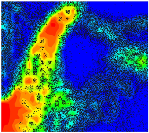
  $\textrm {Kn}_k$, and UGKWP will sample and track the solid particles, keeping the non-equilibrium automatically. On the contrary, in the high concentration region, the high collision frequency between particles means the solid phase is in the equilibrium state, and no particles will be sampled in UGKWP. In the limit of the continuum flow regime with
  $e=1$, the above UGKWP method for (2.1) can recover the solution of the following hydrodynamic equations:
 \begin{align} &\frac{\partial (\epsilon_k\rho_k)}{\partial t} + \boldsymbol{\nabla}_{\boldsymbol{x}} \boldsymbol{\cdot} (\epsilon_k\rho_k \boldsymbol{U}_k) = 0,\end{align}
 \begin{align} &\frac{\partial (\epsilon_k\rho_k \boldsymbol{U}_k)}{\partial t} + \boldsymbol{\nabla}_{\boldsymbol{x}} \boldsymbol{\cdot} (\epsilon_k\rho_k \boldsymbol{U}_k \boldsymbol{U}_k + p_k \mathbb{I} ) = \frac{\epsilon_{k}\rho_{k}(\boldsymbol{U}_g - \boldsymbol{U}_k)}{\tau_{st,k}} \nonumber\\ &\quad - \epsilon_{k} \boldsymbol{\nabla}_{\boldsymbol{x}} p_g + \epsilon_{k}\rho_{k} \boldsymbol{G} + \sum_{i=1,i\neq k}^{N} \beta_{ik}(\boldsymbol{U}_{i}-\boldsymbol{U}_{k}) , \end{align}
 \begin{align} &\frac{\partial (\epsilon_k\rho_k E_k)}{\partial t} + \boldsymbol{\nabla}_{\boldsymbol{x}} \boldsymbol{\cdot} ((\epsilon_k\rho_k E_k + p_{k}) \boldsymbol{U}_k ) = \frac{\epsilon_{k}\rho_{k}\boldsymbol{U}_k \boldsymbol{\cdot} (\boldsymbol{U}_g - \boldsymbol{U}_k)}{\tau_{st,k}} \nonumber\\ &\quad - 3\frac{\epsilon_k\rho_k\theta_k}{\tau_{st,k}} - \epsilon_{k} \boldsymbol{U}_k \boldsymbol{\cdot} \boldsymbol{\nabla}_{\boldsymbol{x}} p_g + \epsilon_{k}\rho_{k} \boldsymbol{U}_k \boldsymbol{\cdot} \boldsymbol{G}. \end{align}
In (2.69),  $p_k$ is the pressure of the
  $k$th disperse solid phase, and it is the sum of the kinetic pressure
  $p_{k,k} = \epsilon _k\rho _k\theta _k$, collisional pressure
  $p_{c,k}$ and frictional pressure
  $p_{f,k}$. Lots of studies about
  $p_{c,k}$ and
  $p_{f,k}$ have been done, especially for the dense particular flow (Dou et al. Reference Dou, Wang, Ge and Ouyang2023). In this paper, the collisional pressure
  $p_{c,k}$ is calculate by
 \begin{equation} p_{c,k} = \sum_{i=1,i\neq k}^{N} p_{c,ik}, \end{equation}
where  $p_{c,ik}$ is the collisional pressure between the
  $i$th and the
  $k$th disperse phases, given in (2.45). The value of
  $p_{f,k}$ accounts for the enduring inter-particle contacts and frictions of the
  $k$th disperse phase, which play important roles when the solid phase is near packing. In this paper, the Johnson–Jackson model is employed (Johnson & Jackson Reference Johnson and Jackson1987; Houim & Oran Reference Houim and Oran2016)
 \begin{equation} p_{f,k} = \left\{\begin{array}{@{}ll} 0, & \epsilon_{t} \le \epsilon_{s,crit}, \\ 0.1 \epsilon_{k} \dfrac{(\epsilon_{t} - \epsilon_{s,crit})^2}{(\epsilon_{s,max} - \epsilon_{t})^5}, & \epsilon_{t} > \epsilon_{s,crit}. \end{array}\right. \end{equation}
Here,  $\epsilon _{s,crit}$ is the critical volume fraction of the whole solid phase. To avoid the solid volume fraction
  $\epsilon _{k}$ exceeding its maximum value
  $\epsilon _{s,max}$, i.e. the over-packing problem, the proposed flux limiting model near the packing condition is employed in the UGKWP method for the solid phase (Yang et al. Reference Yang, Shyy and Xu2022c).
3. Gas-kinetic scheme for gas phase
3.1. Governing equations for gas phase
The gas phase is regarded as the continuum flow and the governing equations are the NS equations with source terms reflecting the inter-phase interaction (Gidaspow Reference Gidaspow1994; Ishii & Hibiki Reference Ishii and Hibiki2006)
 \begin{align} &\frac{\partial (\tilde{\rho}_g)}{\partial t} + \boldsymbol{\nabla}_x \boldsymbol{\cdot} (\tilde{\rho}_g \boldsymbol{U}_g)= 0,\end{align}
 \begin{align} &\frac{\partial (\tilde{\rho}_g \boldsymbol{U}_g)}{\partial t} + \boldsymbol{\nabla}_x \boldsymbol{\cdot} (\tilde{\rho}_g \boldsymbol{U}_g \boldsymbol{U}_g + \widetilde{p_g}\mathbb{I}) - \epsilon_{g} \boldsymbol{\nabla}_x \boldsymbol{\cdot} (\mu_g \boldsymbol{\sigma})\nonumber\\ &\quad = p_g \boldsymbol{\nabla}_x \epsilon_{g} -\sum_{k=1}^{N} \frac{\epsilon_{k}\rho_{k}(\boldsymbol{U}_g - \boldsymbol{U}_k)}{\tau_{st}} + \rho_g \boldsymbol{G}, \end{align}
 \begin{align} &\frac{\partial (\tilde{\rho}_g E_g)}{\partial t} + \boldsymbol{\nabla}_x \boldsymbol{\cdot} ((\tilde{\rho}_g E_g + \widetilde{p_g}) \boldsymbol{U}_g ) - \epsilon_{g} \boldsymbol{\nabla}_x \boldsymbol{\cdot} (\mu_g \boldsymbol{\sigma}\boldsymbol{\cdot}\boldsymbol{U}_g - \kappa \boldsymbol{\nabla}_x T_g ) \nonumber\\ &\quad ={-} p_{g} \frac{\partial \epsilon_{g}}{\partial t} - \sum_{k=1}^{N} \frac{\epsilon_{k}\rho_{k}\boldsymbol{U}_k \boldsymbol{\cdot} (\boldsymbol{U}_g - \boldsymbol{U}_k)}{\tau_{st}} + \sum_{k=1}^{N}\frac{3\epsilon_k\rho_k\theta_k}{\tau_{st}} + \rho_g \boldsymbol{U}_g \boldsymbol{\cdot} \boldsymbol{G}, \end{align}
where  $\tilde {\rho }_g=\epsilon _{g}\rho _g$ is the apparent density of the gas phase,
  $p_g=\rho _gRT_g$ is the pressure of the gas phase and
  $\widetilde {p_g}=\tilde {\rho }_gRT_g$. The strain rate tensor
  $\boldsymbol {\sigma }$ is
 \begin{equation} \boldsymbol{\sigma} = \boldsymbol{\nabla}_x\boldsymbol{U}_g + (\boldsymbol{\nabla}_x\boldsymbol{U}_g)^{\rm T} - \tfrac{2}{3} \boldsymbol{\nabla}_x \boldsymbol{\cdot} \boldsymbol{U}_g \mathbb{I}, \end{equation}
and
 \begin{equation} \mu_g = \tau_{g} p_g,\quad \kappa = \tfrac{5}{2} R \tau_{g} p_g. \end{equation}
In particular, on the right-hand side of (3.1), the term  $p_{g} \boldsymbol {\nabla }_x \epsilon _{g}$ is called the ‘nozzle’ term, and the associated work term
  $- p_{g} ({\partial \epsilon _{g}}/{\partial t})$ is called the
  $pDV$ work term, since it is similar to the
  $pDV$ term in the quasi-one-dimensional gas nozzle flow equations (Houim & Oran Reference Houim and Oran2016). Unphysical pressure fluctuations might occur if the ‘nozzle’ term and
  $pDV$ term are not solved correctly. According to Toro (Reference Toro2013), (3.1) can be written as the following form:
 \begin{align} &\frac{\partial (\rho_g)}{\partial t} + \boldsymbol{\nabla}_x \boldsymbol{\cdot} (\rho_g \boldsymbol{U}_g)= C_{\epsilon_g}\rho_g,\end{align}
 \begin{align} &\frac{\partial (\rho_g \boldsymbol{U}_g)}{\partial t} + \boldsymbol{\nabla}_x \boldsymbol{\cdot} (\rho_g \boldsymbol{U}_g \boldsymbol{U}_g + p_g\mathbb{I} - \mu_g \boldsymbol{\sigma})\nonumber\\ &\quad = C_{\epsilon_g} \rho_g \boldsymbol{U}_g - \sum_{k=1}^{N} \frac{\epsilon_{k}\rho_{k}(\boldsymbol{U}_g - \boldsymbol{U}_k)}{\epsilon_g \tau_{st}} + \frac{\rho_g\boldsymbol{G}}{\epsilon_{g}}, \end{align}
 \begin{align} &\frac{\partial (\rho_g E_g)}{\partial t} + \boldsymbol{\nabla}_x \boldsymbol{\cdot} ((\rho_g E_g + p_g) \boldsymbol{U}_g - \mu_g \boldsymbol{\sigma}\boldsymbol{\cdot}\boldsymbol{U}_g + \kappa \boldsymbol{\nabla}_x T_g) \nonumber\\ &\quad =C_{\epsilon_g} (\rho_g E_g + p_g) - \sum_{k=1}^{N}\frac{\epsilon_{k}\rho_{k}\boldsymbol{U}_k \boldsymbol{\cdot} (\boldsymbol{U}_g - \boldsymbol{U}_k)}{\epsilon_g \tau_{st}} + \sum_{k=1}^{N}\frac{3\epsilon_k\rho_k\theta_k}{\epsilon_g \tau_{st}} + \frac{\rho_g \boldsymbol{U}_g \boldsymbol{\cdot} \boldsymbol{G}}{\epsilon_{g}}, \end{align}
where  $C_{\epsilon _g} = -({1}/{\epsilon _{g}})({\textrm {d}\epsilon _{g}}/{\textrm {d}t})$ with
  ${\textrm {d}\epsilon _{g}}/{\textrm {d}t}={\partial \epsilon _{g}}/{\partial t}+\boldsymbol {U}_g \boldsymbol {\cdot } \boldsymbol {\nabla }\epsilon _{g}$. The method to solve
  $C_{\epsilon _{g}}$ will be introduced later.
3.2. Gas-kinetic scheme for gas evolution
The gas flow is governed by the NS equations with the inter-phase interaction, and its solution will be obtained by the corresponding GKS, which is a limiting scheme of UGKWP in the continuum regime. In general, the evolution of the gas phase (3.4) in one time step  $\Delta t_g$ can be split into three parts
 $$\begin{gather} \mathcal{L}_{g1}:\ \left\{\begin{array}{@{}l} \dfrac{\partial (\rho_g)}{\partial t} + \boldsymbol{\nabla}_x \boldsymbol{\cdot} (\rho_g \boldsymbol{U}_g)= 0, \\ \dfrac{\partial (\rho_g \boldsymbol{U}_g)}{\partial t} + \boldsymbol{\nabla}_x \boldsymbol{\cdot} (\rho_g \boldsymbol{U}_g \boldsymbol{U}_g + p_g\mathbb{I} - \mu_g \boldsymbol{\sigma})= 0,\\ \dfrac{\partial (\rho_g E_g)}{\partial t} + \boldsymbol{\nabla}_x \boldsymbol{\cdot} ((\rho_g E_g + p_g) \boldsymbol{U}_g - \mu_g \boldsymbol{\sigma}\boldsymbol{\cdot}\boldsymbol{U}_g + \kappa \boldsymbol{\nabla}_x T_g ) = 0,\end{array}\right. \end{gather}$$
 $$\begin{gather}\mathcal{L}_{g2}:\ \left\{\begin{array}{@{}l} \dfrac{\partial (\rho_g)}{\partial t} = C_{\epsilon_g}\rho_g, \\ \dfrac{\partial (\rho_g \boldsymbol{U}_g)}{\partial t} = C_{\epsilon_g} \rho_g \boldsymbol{U}_g,\\ \dfrac{\partial (\rho_g E_g)}{\partial t} = C_{\epsilon_g} (\rho_g E_g + p_g). \end{array}\right. \end{gather}$$
 $$\begin{gather}\mathcal{L}_{g3}:\ \left\{\begin{array}{@{}l} \dfrac{\partial (\rho_g)}{\partial t} = 0,\\ \dfrac{\partial (\rho_g \boldsymbol{U}_g)}{\partial t} ={-}\dfrac{\epsilon_{s}\rho_{s}(\boldsymbol{U}_g - \boldsymbol{U}_s)}{\epsilon_g \tau_{st}} + \dfrac{\rho_g\boldsymbol{G}}{\epsilon_{g}}, \\ \dfrac{\partial (\rho_g E_g)}{\partial t} ={-}\dfrac{\epsilon_{s}\rho_{s}\boldsymbol{U}_s \boldsymbol{\cdot} (\boldsymbol{U}_g - \boldsymbol{U}_s)}{\epsilon_g \tau_{st}} + \dfrac{3\epsilon_k\rho_k\theta_k}{\epsilon_g \tau_{st}} + \dfrac{\rho_g \boldsymbol{U}_g \boldsymbol{\cdot} \boldsymbol{G}}{\epsilon_{g}}. \end{array}\right. \end{gather}$$
The variables updated by  $\mathcal {L}_{g1}$,
  $\mathcal {L}_{g2}$ and
  $\mathcal {L}_{g3}$ are denoted as
 \begin{equation} \mathcal{L}_{g1}:\boldsymbol{W}^{n}\to\boldsymbol{W}^{*}, \quad \mathcal{L}_{g2}:\boldsymbol{W}^{*}\to\boldsymbol{W}^{**},\quad \mathcal{L}_{g3}:\boldsymbol{W}^{**}\to\boldsymbol{W}^{n+1}. \end{equation}
Firstly, the kinetic equation without the nozzle and acceleration term  $\mathcal {L}_{g1}$ for
  $\boldsymbol {W}^{n}\to \boldsymbol {W}^{*}$ for the gas phase is modelled by
 \begin{equation} \frac{\partial f_{g}}{\partial t} + \boldsymbol{\nabla}_x \boldsymbol{\cdot} (\boldsymbol{u}f_{g}) = \frac{g_{g}-f_{g}}{\tau_{g}}, \end{equation}
where  $\boldsymbol {u}$ is the velocity,
  $\tau _g$ is the relaxation time for the gas phase,
  $f_{g}$ is the distribution function of the gas phase and
  $g_{g}$ is the corresponding equilibrium state (Maxwellian distribution). The local equilibrium state
  $g_{g}$ can be written as
 \begin{equation} g_{g}=\rho_g\left(\frac{\lambda_g}{\rm \pi}\right)^{{(K+3)}/{2}} {\rm e}^{-\lambda_g[(\boldsymbol{u}-\boldsymbol{U}_g)^2+\boldsymbol{\xi}^2]}, \end{equation}
where  $\rho _g$ is the density,
  $\lambda _g$ is determined by the gas temperature through
  $\lambda _g = {m_g}/{2k_BT_g}$,
  $m_g$ is the molecular mass and
  $\boldsymbol {U}_g$ is the macroscopic velocity of the gas phase. Here,
  $K$ is the internal degree of freedom with
  $K=(5-3\gamma )/(\gamma -1)$ for the three-dimensional diatomic gas, where
  $\gamma =1.4$ is the specific heat ratio. The collision term satisfies the compatibility condition
 \begin{equation} \int \frac{g_g-f_g}{\tau_g} \boldsymbol{\psi} \,\text{d}\varXi=0, \end{equation}
where  $\boldsymbol {\psi }=(1,\boldsymbol {u}, \frac {1}{2}(\boldsymbol {u}^2+\boldsymbol {\xi }^2))^\textrm {T}$, the internal variables
  $\boldsymbol {\xi }^2=\xi _1^2+\cdots +\xi _K^2$ and
  $\textrm {d}\varXi =\textrm {d}\boldsymbol {u}\,\textrm {d}\boldsymbol {\xi }$.
For brevity, the subscript  $g$ will be neglected in this subsection. For (3.9), the integral solution of
  $f$ at the cell interface can be written as
 \begin{equation} f(\boldsymbol{x},t,\boldsymbol{u},\boldsymbol{\xi})=\frac{1}{\tau} \int_0^t g(\boldsymbol{x}',t',\boldsymbol{u},\boldsymbol{\xi})\,{\rm e}^{-(t-t')/\tau}\,\text{d}t' +{\rm e}^{{-}t/\tau}f_0(\boldsymbol{x}-\boldsymbol{u}t,\boldsymbol{u},\boldsymbol{\xi}), \end{equation}
where  $\boldsymbol {x}'=\boldsymbol {x}+\boldsymbol {u}(t'-t)$ is the trajectory of particles,
  $f_0$ is the initial gas distribution function at time
  $t=0$ and
  $g$ is the corresponding equilibrium state. The initial NS gas distribution function
  $f_0$ in (3.12) can be constructed as
 \begin{equation} f_0=f_0^l(\boldsymbol{x},\boldsymbol{u})(1-H(x))+f_0^r(\boldsymbol{x},\boldsymbol{u})H(x), \end{equation}
where  $H(x)$ is the Heaviside function,
  $f_0^l$ and
  $f_0^r$ are the initial gas distribution functions on the left and right sides of one cell interface. More specifically, the initial gas distribution function
  $f_0^k$,
  $k=l,r$, is constructed as
 \begin{equation} f_0^k=g^k(1+\boldsymbol{a}^k \boldsymbol{\cdot} \boldsymbol{x}-\tau(\boldsymbol{a}^k \boldsymbol{\cdot} \boldsymbol{u}+A^k)), \end{equation}
where  $g^l$ and
  $g^r$ are the Maxwellian distribution functions on the left-hand and right-hand sides of a cell interface, which can be fully determined by the macroscopic conservative flow variables
  $\boldsymbol {W}^l$ and
  $\boldsymbol {W}^r$. The coefficients
  $\boldsymbol {a}^l=[a^l_1, a^l_2, a^l_3]^\textrm {T}$ and
  $\boldsymbol {a}^r=[a^r_1, a^r_2, a^r_3]^\textrm {T}$ are related to the spatial derivatives in the normal and tangential directions, which can be evaluated from the corresponding derivatives of the initial macroscopic variables
 \begin{equation} \langle a^l_i\rangle=\partial \boldsymbol{W}^l/\partial x_i,\quad \langle a^r_i\rangle=\partial \boldsymbol{W}^r/\partial x_i, \end{equation}
where  $i=1,2,3$, and
  $\langle \cdots \rangle$ means the moments of the Maxwellian distribution functions
 \begin{equation} \langle\cdots\rangle=\int \boldsymbol{\psi}(\cdots)g\,\text{d}\varXi. \end{equation}
Based on the Chapman–Enskog expansion, the non-equilibrium part of the distribution function satisfies
 \begin{equation} \langle \boldsymbol{a}^l \boldsymbol{\cdot}\boldsymbol{u}+A^l\rangle = 0,\quad \langle \boldsymbol{a}^r \boldsymbol{\cdot}\boldsymbol{u}+A^r\rangle = 0, \end{equation}
and therefore the coefficients  $A^l$ and
  $A^r$ can be fully determined. The equilibrium state
  $g$ around the cell interface is modelled as
 \begin{equation} g=g_0(1+\bar{\boldsymbol{a}}\boldsymbol{\cdot}\boldsymbol{x}+\bar{A}t), \end{equation}
where  $\bar {\boldsymbol {a}}=[\bar {a}_1, \bar {a}_2, \bar {a}_3]^\textrm {T}$,
  $g_0$ is the local equilibrium of the cell interface. More specifically,
  $g$ can be determined by the compatibility condition
 $$\begin{gather} \int\boldsymbol{\psi} g_{0}\,\text{d}\varXi=\boldsymbol{W}_0 =\int_{u>0}\boldsymbol{\psi} g^{l}\,\text{d}\varXi+\int_{u<0}\boldsymbol{\psi} g^{r}\,\text{d}\varXi, \end{gather}$$
 $$\begin{gather}\int\boldsymbol{\psi} \overline{a_i} g_{0}\,\text{d}\varXi=\partial \boldsymbol{W}_0/\partial x_i =\int_{u>0}\boldsymbol{\psi} a^l_i g^{l}\,\text{d}\varXi+\int_{u<0}\boldsymbol{\psi} a^r_i g^{r}\,\text{d}\varXi, \end{gather}$$
 $i=1,2,3$, and
 \begin{equation} \langle \bar{\boldsymbol{a}} \boldsymbol{\cdot} \boldsymbol{u}+\bar{A}\rangle = 0. \end{equation}
After determining all parameters in the initial gas distribution function  $f_0$ and the equilibrium state
  $g$, substituting (3.13) and (3.18) into (3.12), the time-dependent distribution function
  $f(\boldsymbol {x}, t, \boldsymbol {u},\boldsymbol {\xi })$ at a cell interface can be expressed as
 \begin{align} f(\boldsymbol{x}, t, \boldsymbol{u},\boldsymbol{\xi}) &=c_1 g_0+ c_2 \bar{\boldsymbol{a}}\boldsymbol{\cdot}\boldsymbol{u}g_0 +c_3 {\bar{A}} g_0\nonumber\\ &\quad +[c_4 g^r +c_5 \boldsymbol{a}^r\boldsymbol{\cdot}\boldsymbol{u} g^r + c_6 A^r g^r] (1-H(u))\nonumber\\ &\quad+[c_4 g^l +c_5 \boldsymbol{a}^l\boldsymbol{\cdot}\boldsymbol{u} g^l + c_6 A^l g^l] H(u) , \end{align}
with coefficients
 \begin{equation} \left.\begin{array}{c@{}}
c_1 = 1-{\rm e}^{{-}t/\tau}, \\ c_2 = (t+\tau)\,{\rm
e}^{{-}t/\tau}-\tau, \\ c_3 = t-\tau+\tau \,{\rm
e}^{{-}t/\tau}, \\ c_4 = {\rm e}^{{-}t/\tau}, \\ c_5
={-}(t+\tau)\,{\rm e}^{{-}t/\tau}, \\ c_6 ={-}\tau \,{\rm
e}^{{-}t/\tau}. \end{array}\right\}
\end{equation}
\begin{equation} \left.\begin{array}{c@{}}
c_1 = 1-{\rm e}^{{-}t/\tau}, \\ c_2 = (t+\tau)\,{\rm
e}^{{-}t/\tau}-\tau, \\ c_3 = t-\tau+\tau \,{\rm
e}^{{-}t/\tau}, \\ c_4 = {\rm e}^{{-}t/\tau}, \\ c_5
={-}(t+\tau)\,{\rm e}^{{-}t/\tau}, \\ c_6 ={-}\tau \,{\rm
e}^{{-}t/\tau}. \end{array}\right\}
\end{equation}
Then, the flux transport over a time step can be calculated
 \begin{equation} \boldsymbol{F}_{ij} =\int_{0}^{\Delta t} \int\boldsymbol{u}\boldsymbol{\cdot}\boldsymbol{n}_{ij} f_{ij}(\boldsymbol{x},t,\boldsymbol{u},\boldsymbol{\xi})\boldsymbol{\psi}\,\text{d}\varXi\,\text{d}t, \end{equation}
where  $\boldsymbol {n}_{ij}$ is the normal vector of the cell interface. Then, the cell-averaged conservative variables of cell
  $i$ can be updated as follows:
 \begin{equation} \boldsymbol{W}_i^{*} = \boldsymbol{W}_i^n - \frac{1}{\varOmega_i} \sum_{S_{ij}\in \partial \varOmega_i}\boldsymbol{F}_{ij}S_{ij}, \end{equation}
where  $\varOmega _i$ is the volume of cell
  $i$,
$i$,  $\partial \varOmega _i$ denotes the set of the interface of cell
  $i$,
$i$,  $S_{ij}$ is the area of the
  $j$th interface of cell
  $i$,
$i$,  $\boldsymbol {F}_{ij}$ denotes the projected macroscopic fluxes in the normal direction and
  $\boldsymbol {W}_{g}=[\rho _g,\rho _g \boldsymbol {U}_g, \rho _g E_g]^\textrm {T}$ are the cell-averaged conservative flow variables for the gas phase.
In the second part,  $\mathcal {L}_{g2}:\boldsymbol {W}^{*}\to \boldsymbol {W}^{**}$ is about the nozzle term
 \begin{equation}
\left.\begin{array}{c@{}}
\rho_g^{**} = \rho_g^{*} + C_{\epsilon_g}^{*} \rho_g^{*}
\Delta t_g, \\ \rho_g^{**}\boldsymbol{U}_g^{**} =
\rho_g^{*}\boldsymbol{U}_g^{*} + C_{\epsilon_g}^{*}
\rho_g^{*}\boldsymbol{U}_g^{*} \Delta t_g, \\
\rho_g^{**}E_g^{**} = \rho_g^{*}E_g^{*} +
C_{\epsilon_g}^{*} (\rho_g^{*}E_g^{*} + p_g^{*}) \Delta
t_g, \\ \end{array}\right\}
\end{equation}
\begin{equation}
\left.\begin{array}{c@{}}
\rho_g^{**} = \rho_g^{*} + C_{\epsilon_g}^{*} \rho_g^{*}
\Delta t_g, \\ \rho_g^{**}\boldsymbol{U}_g^{**} =
\rho_g^{*}\boldsymbol{U}_g^{*} + C_{\epsilon_g}^{*}
\rho_g^{*}\boldsymbol{U}_g^{*} \Delta t_g, \\
\rho_g^{**}E_g^{**} = \rho_g^{*}E_g^{*} +
C_{\epsilon_g}^{*} (\rho_g^{*}E_g^{*} + p_g^{*}) \Delta
t_g, \\ \end{array}\right\}
\end{equation}
where
 \begin{equation} C_{\epsilon_g}^{*} ={-}\frac{1}{\epsilon_{g}^{n+1}}\left(\frac{\epsilon_{g}^{n+1} - \epsilon_{g}^{n}}{\Delta t_s} + \boldsymbol{U}_g^{*} \boldsymbol{\cdot} \boldsymbol{\nabla}\epsilon_{g}^{n}\right), \end{equation}
with
 \begin{equation} \epsilon_{g}^{n} = 1 - \sum_{k=1}^{N} \epsilon_{k}^{n},\quad \epsilon_{g}^{n+1} = 1 - \sum_{k=1}^{N} \epsilon_{k}^{n+1},\quad \boldsymbol{\nabla}\epsilon_{g}^{n} ={-} \sum_{k=1}^{N} \boldsymbol{\nabla}\epsilon_{k}^{n}. \end{equation}
It is worth noting that  $\boldsymbol {\nabla }\epsilon _{g}$ is the cell-averaged volume fraction gradient of the gas phase in the cell. Taking
  ${\partial \epsilon _{g}}/{\partial x}$ for example, it is calculated by
 \begin{equation} \frac{\partial \epsilon_{g,i}}{\partial x} = \frac{\epsilon_{g,i+{1}/{2}} - \epsilon_{g,i-{1}/{2}}}{\Delta x}, \end{equation}
where  $\epsilon _{g,i-{1}/{2}}$ and
  $\epsilon _{g,i+{1}/{2}}$ are volume fractions of the gas phase at the left and right interfaces of cell
  $i$, which can be obtained from the reconstructed
  $\epsilon _{s}$ at the interface based on
  $\epsilon _{s} + \epsilon _{g} = 1$.
In the third part,  $\mathcal {L}_{g3}:\boldsymbol {W}^{**}\to \boldsymbol {W}^{n+1}$ is for the phase interaction
 \begin{equation} \mathcal{L}_{g3}
:\enspace \left\{\begin{array}{@{}l}
\displaystyle\dfrac{\partial (\rho_g)}{\partial t}= 0, \\
\displaystyle\dfrac{\partial (\rho_g
\boldsymbol{U}_g)}{\partial t} ={-} \sum_{k=1}^{N}
\dfrac{\epsilon_{k}\rho_{k}(\boldsymbol{U}_g -
\boldsymbol{U}_k)}{\epsilon_g \tau_{st}},\\
\displaystyle\dfrac{\partial (\rho_g E_g)}{\partial t} ={-}
\sum_{k=1}^{N}\dfrac{\epsilon_{k}\rho_{k}\boldsymbol{U}_k
\boldsymbol{\cdot} (\boldsymbol{U}_g -
\boldsymbol{U}_k)}{\epsilon_g \tau_{st}} +
\sum_{k=1}^{N}\dfrac{3\epsilon_{k}\rho_k\theta_k}{\epsilon_g
\tau_{st}}, \end{array}\right.
\end{equation}
\begin{equation} \mathcal{L}_{g3}
:\enspace \left\{\begin{array}{@{}l}
\displaystyle\dfrac{\partial (\rho_g)}{\partial t}= 0, \\
\displaystyle\dfrac{\partial (\rho_g
\boldsymbol{U}_g)}{\partial t} ={-} \sum_{k=1}^{N}
\dfrac{\epsilon_{k}\rho_{k}(\boldsymbol{U}_g -
\boldsymbol{U}_k)}{\epsilon_g \tau_{st}},\\
\displaystyle\dfrac{\partial (\rho_g E_g)}{\partial t} ={-}
\sum_{k=1}^{N}\dfrac{\epsilon_{k}\rho_{k}\boldsymbol{U}_k
\boldsymbol{\cdot} (\boldsymbol{U}_g -
\boldsymbol{U}_k)}{\epsilon_g \tau_{st}} +
\sum_{k=1}^{N}\dfrac{3\epsilon_{k}\rho_k\theta_k}{\epsilon_g
\tau_{st}}, \end{array}\right.
\end{equation}
Obviously, we have  $\rho _g^{n+1}=\rho _g^{**}$. Then, the second equation represents the momentum exchange between the gas phase with multi-disperse phases
 \begin{equation} \frac{\partial (\rho_g \boldsymbol{U}_g)}{\partial t} ={-} \sum_{k=1}^{N} \frac{\epsilon_{k}\rho_{k}(\boldsymbol{U}_g - \boldsymbol{U}_k)}{\epsilon_g \tau_{st}} \overset{def}{=} - \frac{1}{\epsilon_g} \beta_t(\boldsymbol{U}_g - \boldsymbol{U}_t), \end{equation}
where  $\beta _{t}$ and
  $\boldsymbol {U}_t$ are the equivalent momentum transfer coefficient and velocity of the whole solid phase
 \begin{equation} \beta_t \overset{def}{=} \sum_{k=1}^{N}\beta_k = \sum_{k=1}^{N}\frac{\epsilon_{k} \rho_{k}}{\tau_{st,k}}, \quad \boldsymbol{U}_t \overset{def}{=} \sum_{k=1}^{N} \frac{\beta_k \boldsymbol{U}_k}{\beta_t}. \end{equation}
The calculations of  $\beta _t$ and
  $\boldsymbol {U}_k$ are based on the variables of the
  $n+1$ state of the solid phase. For the above equation, the analytical solution of
  $\boldsymbol {U}_g$ can be obtained
 \begin{equation} \boldsymbol{U}_g^{n+1} = \boldsymbol{U}_t^{n+1} + (\boldsymbol{U}_g^{**} - \boldsymbol{U}_t^{n+1}) \,{\rm e}^{-({\beta_t^{n+1} \Delta t_g}/{\epsilon_{g}^{n+1} \rho_g^{n+1}})}. \end{equation}
Finally, the energy of the gas phase can be updated by
 \begin{align}
\rho_g^{n+1}E_g^{n+1} \,{=}\, \rho_g^{**}E_g^{**} \,{-} \left[
\sum_{k=1}^{N}\frac{1}{\epsilon_g^{n+1}} \beta_k^{n+1}
\boldsymbol{U}_k^{n+1} \boldsymbol{\cdot}
(\boldsymbol{U}_g^{n+1} - \boldsymbol{U}_k^{n+1})
-\sum_{k=1}^{N}\frac{3\epsilon_k^{n+1}\rho_k\theta_k^{n+1}}{\epsilon_g^{n+1}
\tau_{st}} \right] \Delta t_g.
\end{align}
\begin{align}
\rho_g^{n+1}E_g^{n+1} \,{=}\, \rho_g^{**}E_g^{**} \,{-} \left[
\sum_{k=1}^{N}\frac{1}{\epsilon_g^{n+1}} \beta_k^{n+1}
\boldsymbol{U}_k^{n+1} \boldsymbol{\cdot}
(\boldsymbol{U}_g^{n+1} - \boldsymbol{U}_k^{n+1})
-\sum_{k=1}^{N}\frac{3\epsilon_k^{n+1}\rho_k\theta_k^{n+1}}{\epsilon_g^{n+1}
\tau_{st}} \right] \Delta t_g.
\end{align}
Now, the evolution of the gas phase in  $\Delta t_g$ is finished.
In the evolution,  $\Delta t_{s,k}$ and
  $\Delta t_g$ will be calculated based on the Courant–Friedrichs–Lewy (CFL) condition; the solid phase will be updated firstly by one solid time step
  $\Delta t_s = \min (\Delta t_{s,k})$; then, the gas phase will be updated based on the gas time step
  $\Delta t_g$ until
  $\sum _i \Delta t_{g,i} = \Delta t_s$, and the evolution of gas-particle two-phase flow in
  $\Delta t_s$ will be finished. The flow chart of GKS-UGKWP for polydisperse gas-particle flow is given in figure 1, and the main difference from the monodisperse counterpart is the calculation of solid phase, marked by the blue box.
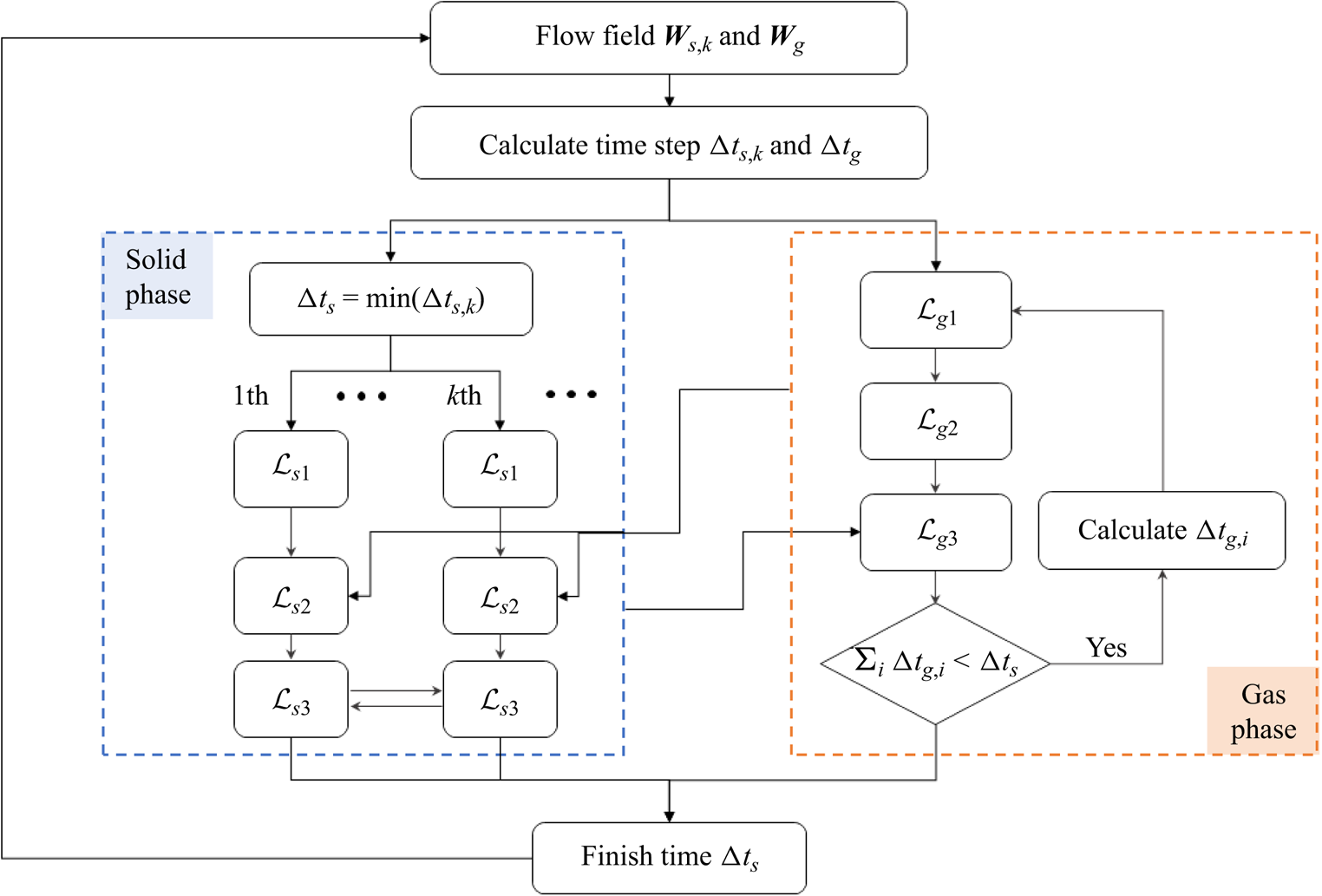
Figure 1. The flow chart of GKS-UGKWP method for polydisperse gas-particle two-phase flow.
4. Numerical simulations
4.1. Circulating fluidized bed
4.1.1. Case description
The first case is a circulating fluidized bed (CFB) with two disperse solid phases (Niemi Reference Niemi2012; Wang et al. Reference Wang, Niemi, Peltola, Kallio, Yang, Lu and Wei2015). The experiment data will be used to validate the GKS-UGKWP method. As in previous studies (Wang et al. Reference Wang, Niemi, Peltola, Kallio, Yang, Lu and Wei2015), a two-dimensional domain with  $D\times H=0.4\ \textrm {m}\times 3\ \textrm {m}$ is employed in this paper. The uniform rectangular mesh is used in the whole domain with mesh number
  $66\times 500$, and correspondingly the cell size
  $\varDelta _x \approx \varDelta _y = 6\times 10^{-3}\ \textrm {m}$. According to the experiment measurement (Niemi Reference Niemi2012), the total inventory of solid particles is 2.85 kg, and the mass fraction, diameter and material density of each disperse phase are listed in table 1. The maximum solid volume fraction is taken as
  $\epsilon _{t,max} = 0.55$ in this case. Initially, the solid phase is uniformly distributed in the whole domain, and according to the mass shown in table 1, the initial solid volume fractions are
  $\epsilon _{1}=0.0498$ and
  $\epsilon _{2}=0.0140$, with the assumption of a riser thickness of
  $T=1.5$ cm, which is the same as the value employed in Wang et al. (Reference Wang, Niemi, Peltola, Kallio, Yang, Lu and Wei2015). In the simulation, the solid particles are free to leave the domain at the top boundary. To simplify the simulation, the left and right boundaries are fixed walls, and thus the escaped solid particles will be replenished in the computational domain from the bottom boundary, instead of opening the right boundary as adopted in Wang et al. (Reference Wang, Niemi, Peltola, Kallio, Yang, Lu and Wei2015). A gas with velocity
  $U_g=2.25$ m s
 $^{-1}$ flows into the domain through the bottom boundary to fluidize the solid particles. For the left and right wall boundaries, the mixed wall boundary condition, shown in Appendix A, and no-slip wall boundary condition are used for the solid phase and gas phase, respectively. For this case, the widely used drag correlation proposed by Gibilaro is employed for both disperse phases (Gibilaro et al. Reference Gibilaro, Di Felice, Waldram and Foscolo1985; Mckeen & Pugsley Reference Mckeen and Pugsley2003), which can be written as
 \begin{equation} \beta_{k} = \left(\frac{17.3}{Re_{s,k}}+0.336\right) \frac{\rho_g |\boldsymbol{U}_g-\boldsymbol{u}_k|}{d_k} \epsilon_{k}\epsilon_{g}^{{-}1.8}, \end{equation}
where  $Re_{s,k}={\epsilon _{g}\rho _g d_k |\boldsymbol {U}_g - \boldsymbol {u}_k|}/{\mu _g}$ is the Reynolds number (Re) of the
  $k$th disperse solid phase. It is worth noting that for each disperse phase,
  $\tau _{st,k}$ can be obtained by the relation
  $\beta _{k}={\epsilon _{k} \rho _k}/{\tau _{st,k}}$.
Table 1. The properties of the solid particles for the CFB case (Niemi Reference Niemi2012).

4.1.2. Results
In this case, the simulation time is  $10.0$ s, and the results from
  $6.0$ to
  $10.0$ s are used for the averaging. Physically, to study the flow properties at different vertical positions in the riser, four gauges are set at
  $h=0.32$, 0.40, 0.80, 1.20 m in the experiment. Numerically, the total solid volume fraction
  $\epsilon _{t}$ and the overall vertical velocity of solid phase
  $U_s$ at the above four heights are averaged and compared with experimental measurements in figure 2. Note that the overall vertical velocity of the whole solid phase
  $U_s$ is obtained by the individual velocities weighted by solid volume fractions,
  $U_s=\sum _{k}\epsilon _k U_{s,k}/\sum _{k} \epsilon _k$. The mesh is further refined to
  $80 \times 600$ grid points, and the time-averaged results of
  $\epsilon _{t}$ and
  $U_s$ are shown in figure 3. Similar results have been obtained from the refined mesh in comparison with those in figure 2, and therefore the following analysis is based on the coarser mesh with
  $66 \times 500$ points only.
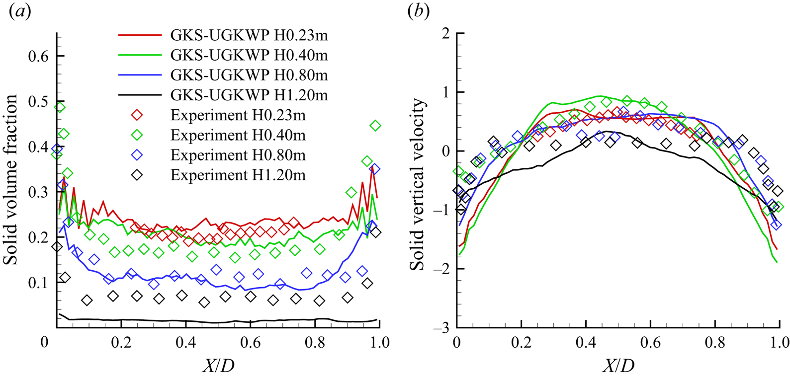
Figure 2. The profiles of  $(a)$ time-averaged total solid volume fraction
  $\epsilon _{t}$ and
  $(b)$ time-averaged overall vertical velocity of solid phase
  $U_s$ at different riser heights by GKS-UGKWP method with a total
  $66 \times 500$ mesh points and the comparison with the experimental measurements.
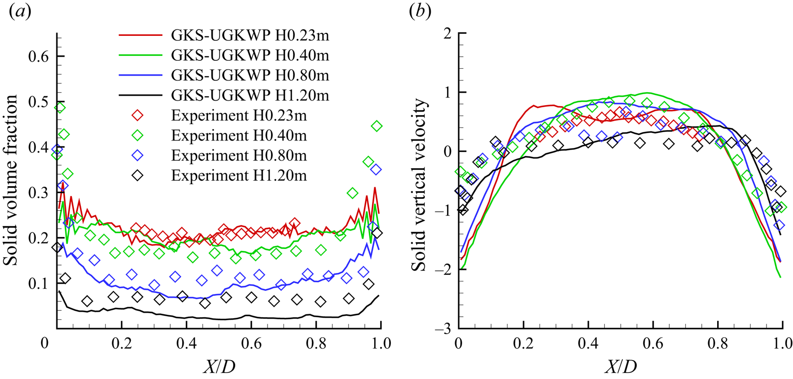
Figure 3. The profiles of  $(a)$ time-averaged total solid volume fraction
  $\epsilon _{t}$ and
  $(b)$ time-averaged overall vertical velocity of solid phase
  $U_s$ at different riser heights by GKS-UGKWP method with a total
  $80 \times 600$ mesh points and the comparison with the experimental measurements.
Figure 2 shows that the numerical results by the GKS-UGKWP method basically agree with the experiment measurements, validating the reliability and accuracy of the proposed method. At  $h=1.20$ m, the computational results
  $\epsilon _t \simeq 2\,\%\unicode{x2013} 3\,\%$ are somehow lower than the experiment values
  $\simeq$6 %, which may be due to the boundary treatment, such that the escaped particles from the top boundary are replenished at the bottom boundary, but not from the sidewalls. The choices of drag model will affect the solution as well. As described in the introduction, the drag model with the consideration of mesoscopic sub-grid flow structures performs better than the traditional homogeneous drag model (Wang & Li Reference Wang and Li2007; Zhu et al. Reference Zhu, Ouyang, Lei and Luo2021). The current method may give better prediction around
  $h=1.20$ m if the mesoscale drag model is employed, which will be studied in the future. In experiment, it is usually assumed that the solid concentration is the same as the pressure gradient along the vertical riser, i.e.
  $\epsilon _{s} \cong -{(\partial p_g / \partial y)}/{\rho _{s} G}$. Here, the predicted
  $\epsilon _t$ evaluated by the time-averaged pressure gradient is also presented in figure 4. Compared with figure 2(a), the solid concentration values by these two approaches show some deviations in the bottom dense regions, i.e.
  $h=0.23$, 0.40 m, but agree well in other regions, i.e.
  $h=0.80$, 1.20 m.

Figure 4. The profiles of solid volume fraction evaluated from the time-averaged pressure gradient,  $\epsilon _{t} = -{(\partial p_g / \partial y)}/{\rho _{s} G}$, at different riser heights by GKS-UGKWP method and the comparison with the experimental measurements.
Besides, the snapshots of solid particles  $\epsilon _{t}$ at different times are presented in figure 5. In general, the solid particles prefer to accumulate at the riser's bottom and near the wall, resulting in a relatively higher concentration in these zones. Furthermore, the instantaneous results clearly show the instantaneously coexisting and dynamically intervening dilute/dense flow regions. The spatially evolving solid volume fraction can be hardly captured smoothly by the hybrid EE/EL methods. The above characteristics are also found in the studies of monodisperse CFB cases.

Figure 5. The instantaneous snapshots of total solid volume fraction  $\epsilon _{t}$ at (a)
  $t=6.0$ s, (b)
  $t=7.0$ s, (c)
  $t=8.0$ s, (d)
  $t=9.0$ s and (e)
  $t=10.0$ s.
For each disperse solid phase,  $\textrm {Kn}_k$, defined by
  $\textrm {Kn}_k={\tau _k}/{\Delta t_s}$ with the local collision time
  $\tau _k$ of the
  $k$th disperse phase, is presented in figure 6. Distributed by
  $\textrm {Kn}_k$, the wave component, contour of
  $\epsilon ^{wave}_k$ and the particle component, the set of sampled particles coloured by their vertical velocity
  $P_k$, are also shown in figure 6. Note that the sum of the wave
  $\epsilon _{k}^{wave}$ and the solid particle
  $P_k$ components is equal to
  $\epsilon _{k}$, as shown in figure 6. The vertical velocity of each solid phase
  $U_{s,k}$ is also given in figure 6. The spatial distributions of
  $\epsilon$ and
  $U_s$ of two particle phases are distinguishable, indicating the necessity of the polydisperse method. For both solid phases, Kn is generally smaller in the near-bottom and near-wall zones of the riser due to the accumulation and collisions of particles in these regions. The two disperse solid particle phases adjust their weights to the wave and particle components in UGKWP according to their respective Kn. One obvious advantage of the GKS-UGKWP for polydisperse flow is that each disperse phase can take the independent wave and particle decompositions.

Figure 6. The instantaneous snapshots of Kn, solid volume fraction  $\epsilon$, solid volume fraction by wave in UGKWP
  $\epsilon ^{wave}$, the set of sampled particles in UGKWP
  $P$ and the vertical velocity of solid phase
  $U_s$ at
  $t=8.0$ s: (a)
  $\textrm {Kn}_1$, (b)
  $\epsilon _1$, (c)
  $\epsilon ^{wave}_1$, (d)
  $P_1$, (e)
  $U_{s,1}$, (f)
  $\textrm {Kn}_2$, (g)
  $\epsilon _2$, (h)
  $\epsilon ^{wave}_2$, (i)
  $P_2$, (j)
  $U_{s,2}$. The figures with subscript 1 are the results of the
  $1$st solid phase (small particle), and the figures with subscript 2 are the results of the
  $2$nd solid phase (large particle). The value of
  $\textrm {Kn}_k$ is coloured by the Kn-legend. The solid volume fraction
  $\epsilon _k$ and the corresponding wave component
  $\epsilon ^{wave}_k$ are coloured by the eps-legend. The discrete particles in particle set
  $P_k$ and the vertical velocity of solid phase
  $U_{s,k}$ are coloured by the Us-legend, with
  $k=1,2$. The legend of Kn is in the exponential distribution. Note that the sum of
  $\epsilon _{1}$ and
  $\epsilon _{2}$ is exactly equal to
  $\epsilon _{t}$ at
  $t=8.0$ s, as shown in figure 5.
4.2. Turbulent fluidized bed
4.2.1. Case description
The dense turbulent fluidized bed (TFB) was applied in the petroleum refining industry and was studied experimentally and numerically (Gao et al. Reference Gao, Lan, Fan, Chang, Wang, Lu and Xu2009; Li et al. Reference Li, Lan, Xu, Wang, Lu and Gao2009). In this problem, two kinds of particles, such as the fluid catalytic cracking (FCC) catalyst (fine) and millet (coarse), are involved with detailed properties given in table 2. Table 2 shows that the densities of two types of particles are very close, while the particle sizes are very different. This flow condition brings challenges to the numerical methods for the gas-particle system with a single solid phase alone, where the tracking of multiple solid phases in GKS-UGKWP seems suitable for this problem. The case of initial bed height  $H_0 = 1.155$ m and gas velocity
  $U_g=0.53$ m s
 $^{-1}$ is studied in this paper. The computational domain is
  $D\times H=0.5\ \textrm {m} \times 4\ \textrm {m}$ and is covered by a uniform rectangular mesh
  $40\times 300$. The maximum solid volume fraction is taken as
  $\epsilon _{s,max}=0.65$ in this study. At the beginning of the simulation, all solid particles are uniformly distributed in the whole riser with initial volume fraction
  $\epsilon _{1}=0.118$ and
  $\epsilon _{2}=0.070$ for the small and large particle phases, respectively. The solid particles escaping from the top boundary will be recirculated back to the computational domain through the bottom boundary. For the gas phase, the standard atmospheric condition is employed at the top boundary, and the gas blows into the riser through the bottom boundary with the velocity
  $U_g$ and a pressure difference of
  $\Delta p = \epsilon _{s,max} (\rho _s^* -\rho _g) GH_0$ from the top boundary, where
  $\rho _s^*=1463.3$ kg m
 $^{-3}$ is the density of the solid particles weighted by their initial volume fractions. The same as the above CFB case, the mixed boundary condition and no-slip wall boundary condition are employed on the sidewalls for the particle phase and gas phase, respectively.
Table 2. The properties of fine and coarse particles in TFB (Gao et al. Reference Gao, Lan, Fan, Chang, Wang, Lu and Xu2009).
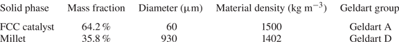
In GKS-UGKWP, each solid phase can choose the most accurate and suitable drag model for the polydisperse system. As shown in table 2, the fine and coarse particles are the Geldart A and D groups, respectively, and different drag models are employed to evaluate the gas–solid interaction in the FCC catalyst and millet particle phases. Different drag models and their modifications are studied and compared (Gao et al. Reference Gao, Lan, Fan, Chang, Wang, Lu and Xu2009). More specifically, for the coarse particle, the Gidaspow model is used (Gidaspow Reference Gidaspow1994)
 \begin{align}
\beta_{k}=\left\{\begin{array}{@{}ll} \displaystyle
150\dfrac{\epsilon_{k} (1-\epsilon_{g}) \mu_g}{\epsilon_{g}
d_k^2} + 1.75\dfrac{\epsilon_{k}\rho_g |\boldsymbol{U}_g -
\boldsymbol{u}_k|}{d_k}, & \epsilon_{g} \le 0.8,\\
\displaystyle \dfrac{3}{4}C_d(Re_{s,k})
\dfrac{\epsilon_{k}\epsilon_{g}\rho_g}{d_k}|\boldsymbol{U}_g-\boldsymbol{u}_k|
\epsilon_{g}^{{-}2.65}, & \epsilon_{g} > 0.8,
\end{array}\right. \end{align}
\begin{align}
\beta_{k}=\left\{\begin{array}{@{}ll} \displaystyle
150\dfrac{\epsilon_{k} (1-\epsilon_{g}) \mu_g}{\epsilon_{g}
d_k^2} + 1.75\dfrac{\epsilon_{k}\rho_g |\boldsymbol{U}_g -
\boldsymbol{u}_k|}{d_k}, & \epsilon_{g} \le 0.8,\\
\displaystyle \dfrac{3}{4}C_d(Re_{s,k})
\dfrac{\epsilon_{k}\epsilon_{g}\rho_g}{d_k}|\boldsymbol{U}_g-\boldsymbol{u}_k|
\epsilon_{g}^{{-}2.65}, & \epsilon_{g} > 0.8,
\end{array}\right. \end{align}
while, for the fine FCC catalyst particles, the four-zone drag model is employed
 \begin{equation}
\beta_{k}=\left\{\begin{array}{@{}ll} \displaystyle
150\dfrac{\epsilon_{k} (1-\epsilon_{g}) \mu_g}{\epsilon_{g}
(d_k^*)^2} + 1.75\dfrac{\epsilon_{k}\rho_g
|\boldsymbol{U}_g - \boldsymbol{u}_k|}{d_k^*}, & 0 \le
\epsilon_{g} \le 0.8,\\ \displaystyle
\dfrac{5}{72}C_d(Re_{s,k}^*)\dfrac{\epsilon_{k}\epsilon_{g}\rho_g}{d_k^*(1
- \epsilon_{g})^{0.293}
}|\boldsymbol{U}_g-\boldsymbol{u}_k|, & 0.8 < \epsilon_{g}
\le 0.933,\\ \displaystyle \dfrac{3}{4}C_d(Re_{s,k})
\dfrac{\epsilon_{k}\epsilon_{g}\rho_g}{d_k}|\boldsymbol{U}_g-\boldsymbol{u}_k|
\epsilon_{g}^{{-}2.65}, & 0.933 < \epsilon_{g} \le 0.990,\\
\displaystyle \dfrac{3}{4}C_d(Re_{s,k})
\dfrac{\epsilon_{k}\rho_g}{d_k}|\boldsymbol{U}_g-\boldsymbol{u}_k|,
& 0.990 < \epsilon_{g} \le 1.0, \end{array}\right.
\end{equation}
\begin{equation}
\beta_{k}=\left\{\begin{array}{@{}ll} \displaystyle
150\dfrac{\epsilon_{k} (1-\epsilon_{g}) \mu_g}{\epsilon_{g}
(d_k^*)^2} + 1.75\dfrac{\epsilon_{k}\rho_g
|\boldsymbol{U}_g - \boldsymbol{u}_k|}{d_k^*}, & 0 \le
\epsilon_{g} \le 0.8,\\ \displaystyle
\dfrac{5}{72}C_d(Re_{s,k}^*)\dfrac{\epsilon_{k}\epsilon_{g}\rho_g}{d_k^*(1
- \epsilon_{g})^{0.293}
}|\boldsymbol{U}_g-\boldsymbol{u}_k|, & 0.8 < \epsilon_{g}
\le 0.933,\\ \displaystyle \dfrac{3}{4}C_d(Re_{s,k})
\dfrac{\epsilon_{k}\epsilon_{g}\rho_g}{d_k}|\boldsymbol{U}_g-\boldsymbol{u}_k|
\epsilon_{g}^{{-}2.65}, & 0.933 < \epsilon_{g} \le 0.990,\\
\displaystyle \dfrac{3}{4}C_d(Re_{s,k})
\dfrac{\epsilon_{k}\rho_g}{d_k}|\boldsymbol{U}_g-\boldsymbol{u}_k|,
& 0.990 < \epsilon_{g} \le 1.0, \end{array}\right.
\end{equation}
where  $d_k$ is the diameter of the solid particle and
  $d_k^*$ in (4.3) is the effective diameter of the FCC catalyst phase, taken as
  $300\mu m$ for better agreement with experimental measurement (Gao et al. Reference Gao, Lan, Fan, Chang, Wang, Lu and Xu2009; Li et al. Reference Li, Lan, Xu, Wang, Lu and Gao2009). The proposed drag model in (4.3) has fully considered the effect of the particles’ clusters, which is also employed in this paper. Besides, in (4.2) and (4.3),
  $C_d$ and
  $Re_{s,k}$ are defined as below
 \begin{equation} C_d (Re_k)
=\left\{\begin{array}{@{}ll} \dfrac{24}{Re_k}(1 +
0.15Re_k^{0.687}), & Re_k \le 1000,\\ 0.44, & Re_k > 1000,
\end{array}\right. \end{equation}
\begin{equation} C_d (Re_k)
=\left\{\begin{array}{@{}ll} \dfrac{24}{Re_k}(1 +
0.15Re_k^{0.687}), & Re_k \le 1000,\\ 0.44, & Re_k > 1000,
\end{array}\right. \end{equation}
and
 \begin{equation} Re_{s,k} = \frac{\epsilon_{g}\rho_g d_k |\boldsymbol{U}_g - \boldsymbol{u}_k|}{\mu_g}, \quad Re_{s,k}^{*} = \frac{\epsilon_{g}\rho_g d_k^* |\boldsymbol{U}_g - \boldsymbol{u}_k|}{\mu_g}. \end{equation}
4.2.2. Results
The time-averaged results from 10.0 to 15.0 s are shown in figure 7. The solid phase in the riser shows higher concentration at the bottom zone and lower density in the top zone, and a sharp transition occurs in a very small region around 1.7–2.0 m. Overall, the predicted apparent density of the solid phase agrees well with the experimental measurements. It is worth mentioning that the choice of a reasonable and accurate drag model which involves the subgrid information is very important for the accurate prediction in numerical simulation (Wang & Li Reference Wang and Li2007; Zhu et al. Reference Zhu, Ouyang, Lei and Luo2021). Besides, figure 7 also presents profiles of  $\epsilon$ for two solid phases and shows a similar trend along the riser height.
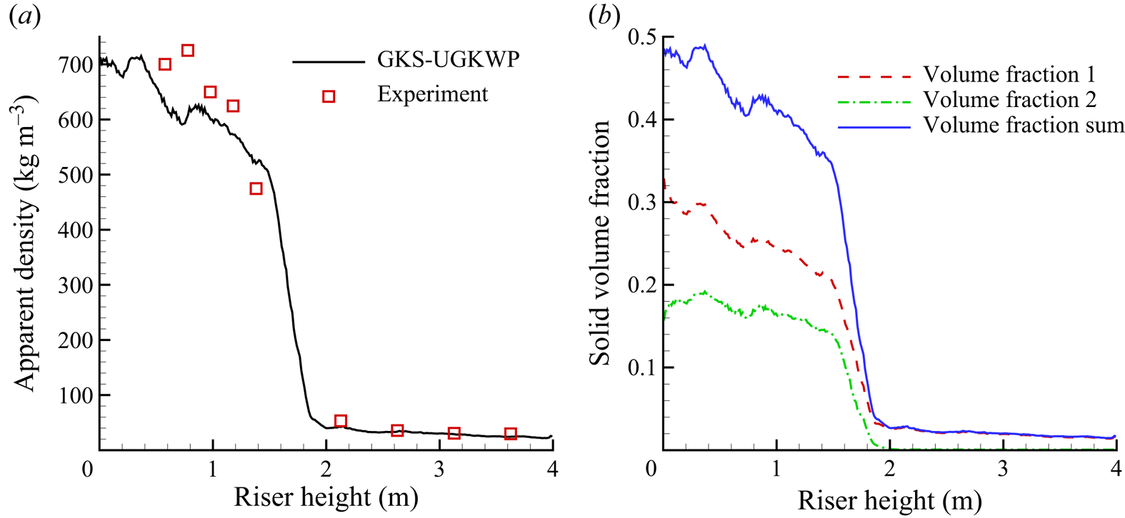
Figure 7. (a) The profiles of time-averaged apparent density of whole solid phase  $\sum _{k}\epsilon _{k}\rho _{k}$ along the riser height by GKS-UGKWP method and comparison with experimental measurements. (b) The profiles of time-averaged solid volume fraction of each disperse phase
  $\epsilon _{k}$,
  $k=1,2$ and their sum
  $\epsilon _{t}$.
The instantaneous snapshots of the solid phase density,  $\sum _{k}\epsilon _{k}\rho _{k}$ in the range
  $10.0\unicode{x2013} 15.0$ s are given in figure 8, which indicates a typical feature of TFB. The coexistence pattern of bottom dense/middle transition/up dilute regions is well captured. All solid particles in the top dilute region are FCC catalyst (Geldart A) type. Figure 8 shows the particle-cluster phenomenon, which has difficulty in the drag modelling in these regions. In the bottom dense region, the gas bubble with variable solid particles inside shows a complex pattern and its tangling with the dense solid phase.
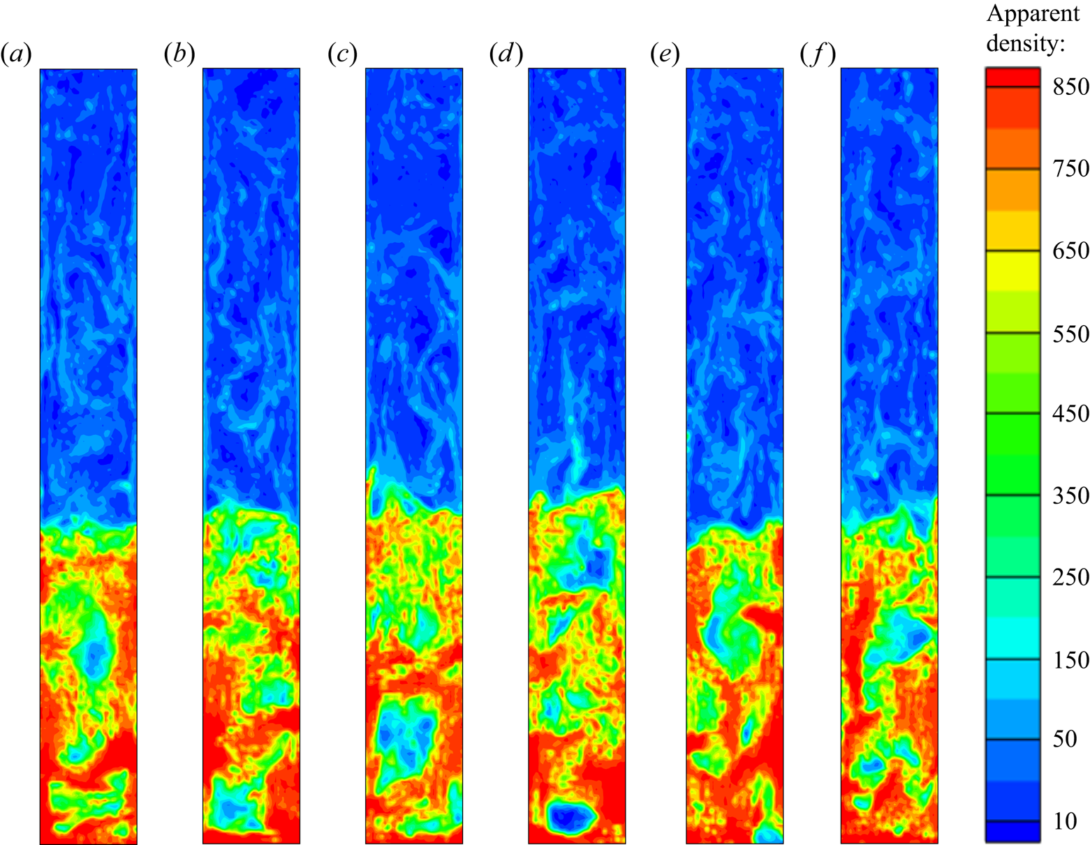
Figure 8. The instantaneous snapshots of apparent density of the whole solid phase  $\sum _{k}\epsilon _{k}\rho _{k}$ at (a)
  $t=10.0$ s, (b)
  $t=11.0$ s, (c)
  $t=12.0$ s, (d)
  $t=13.0$ s, (e)
  $t=14.0$ s and (f)
  $t=15.0$ s.
Since the diameters of two solid phases (60 and 930  $\mathrm {\mu }$m) have a
  $15$ times difference, it is interesting to present their respective distributions. Figure 9 shows the apparent density of each phase
  $\epsilon _{k}\rho _{k}$,
  $k=1,2$ at
  $t=11.0$ s. The summation
  $\sum _{k}\epsilon _{k}\rho _{k}$ is exactly the apparent density at 11.0 s in figure 8(b). The obvious characteristic feature is that, in the up-dilute regions, only the smaller (FCC catalyst) particles exist without millet particles, as shown in the time-averaged profile of
  $\epsilon$ of figure 7. Also, for both solid phases at
  $h\approx 1.7$ m, there is a separation zone with a large Kn above and a small Kn below. Compared with the FFC catalyst phase, the millet phase shows a strong non-equilibrium with a large Kn in the bottom dense region. The decompositions of wave and particle, determined by the local Kn, are presented in figure 9 through the contoured apparent density
  $\epsilon _{k}\rho _{k}$ and scattered particle set
  $P_k$. For the FCC catalyst phase, the Lagrangian particle fully determines its evolution in the up-dilute region, while the wave component is dominant in the bottom region with tremendous amount of real particles and their collisions. For the millet large particle phase, even in the bottom dense region, lots of particles are sampled and tracked in its evolution.
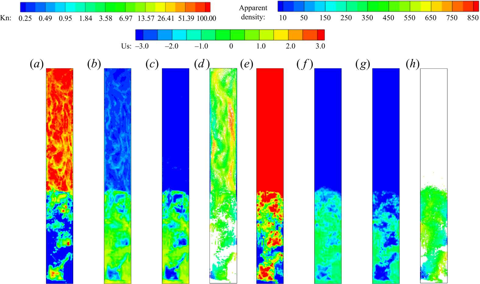
Figure 9. The instantaneous snapshots of  $\textrm {Kn}_k$, solid apparent density
  $\epsilon _k\rho _k$, solid apparent density by wave in UGKWP
  $\epsilon ^{wave}_k\rho _k$ and the set of sampled particles in UGKWP
  $P_k$ at
  $t=11.0$ s: (a)
  $\textrm {Kn}_1$, (b)
  $\epsilon _1\rho _1$, (c)
  $\epsilon ^{wave}_1\rho _1$, (d)
  $P_1$, (e)
  $\textrm {Kn}_2$, (f)
  $\epsilon _2\rho _2$, (g)
  $\epsilon ^{wave}_2\rho _2$ and (h)
  $P_2$. The subscripts 1 and 2 stand for the
  $1$st (FCC catalyst particle) solid phase and the
  $2$nd (millet particle) solid phase, respectively. The
  $\textrm {Kn}_k$ is coloured by the Kn-legend, the solid apparent density
  $\epsilon _k\rho _k$ and wave component
  $\epsilon ^{wave}_k\rho _k$ are coloured by the legend of apparent density and the discrete particles in particle set
  $P_k$ are coloured by the Us-legend (vertical velocity of the solid particle), with
  $k=1,2$. The legend of Kn is in an exponential distribution.
It is necessary to understand the flow properties related to the dilute/dense and non-equilibrium/equilibrium in the gas-particle system. The dilute or dense flow is generally determined by the solid volume fraction, while non-equilibrium/equilibrium is determined by the Kn of the solid particle phase. The dilute and dense flow regions can be associated with either non-equilibrium and equilibrium regimes, especially for the dense particle flow, with many differences in their particle diameters or material density. In UGKWP, Kn is used to determine the decomposition of wave and particle according to the extent of local non-equilibrium. The snapshots of Kn for each disperse phase at different times are shown in figure 10. For both disperse phases, in the bottom dense region at  $h<1.7$ m the non-equilibrium/equilibrium regimes are not spatially fixed and become dynamically inter-convertible. The proposed GKS-UGKWP for polydisperse flow is suitable to treat each individual solid phase with the optimal decompositions of wave and particle.

Figure 10. The instantaneous snapshots of Kn of FCC catalyst particle phase at different times: (a)  $t=10$ s, (b)
  $t=12$ s, (c)
  $t=14$ s and (d)
  $t=15$ s. The instantaneous snapshots of Kn of millet particle phase at different times: (e)
  $t=10$ s, (f)
  $t=12$ s, (g)
  $t=14$ s and (h)
  $t=15$ s. The legend of Kn is in an exponential distribution.
4.3. Interaction of a shock wave with a dense particle curtain
4.3.1. Case description
The interaction of a shock wave with a solid particle bed is a highly challenging problem for a numerical method to be capable of capturing the shock wave propagation at supersonic speed and calculating the gas–solid phase interaction and particle–particle collisions at moderate/dense cases (Ling et al. Reference Ling, Wagner, Beresh, Kearney and Balachandar2012; Tian et al. Reference Tian, Zeng, Meng, Chen, Guo and Xue2020). Here, the interaction of a planar shock with a particle curtain is studied by the GKS-UGKWP method in two-dimensional space, and the simulation solution is compared with the experimental measurement (Ling et al. Reference Ling, Wagner, Beresh, Kearney and Balachandar2012). As sketched in figure 11(a), a planar shock with Mach number  $(\text{Ma})=1.66$ in the gas tube moves from the left to the right (
 $x$ direction), and encounters an initially stationary particle curtain with a width of
  $L=2$ mm. Starting from the impingement of the shock on the solid particles bed, a reflecting shock moving to the left and a transmitting shock moving to the right will occur. Simultaneously, driven by the high-speed gas flow, the solid particles will move to the right by following the transmitted shock front. The computational domain
  $X\times Y$ is
  $[-0.375 \textrm {m}, 0.125\ \textrm {m}] \times [-0.04\ \textrm {m}, 0.04\ \textrm {m}]$ and is covered by a uniform rectangular mesh with
  $1000\times 160$ cells. In the experiment, the diameter of solid particles is distributed by
  $106\unicode{x2013} 125\ \mathrm {\mu } \textrm {m}$. While in the computation, the simulation is based on two disperse phases with solid particle diameters
  $d_1=110$
  $\mathrm {\mu }$m and
  $d_2=120$
  $\mathrm {\mu }$m. The material density of all solid particles is
  $\rho _s = 2520$ kg m
 $^{-3}$ with the restitution coefficient
  $e=0.95$. Initially, the solid particles are uniformly distributed with
  $\epsilon _{1}=0.105$ and
  $\epsilon _{2}=0.105$. The initial state of the gas phase in the domain is the same as the experiment:
  $p_{g,1}=8.27\times 10^{4}\ \textrm {Pa}$,
  $U_{g,1}=0$ m s
 $^{-1}$ and
  $T_{g,1}=296.40$ K, with gas constant
  $R=287.05$ J (kg K)
 $^{-1}$ and specific heat ratio
  $\gamma =1.4$. At the left boundary, the pre-shock condition at
  $\textrm {Ma}=1.66$ is given by
  $p_{g,2}=2.52\times 10^{5}$ Pa,
  $U_{g,2}=304.16$ m s
 $^{-1}$ and
  $T_{g,2}=423.79$ K. The free boundary condition is employed at the right boundary. Besides, for the top and bottom boundaries, the no-slip and slip boundary condition are taken for the gas and solid particle phases, respectively. To monitor the pressure of the gas flow, two gauge positions are set at
  $68.6$ mm upstream and
  $64.2$ mm downstream of the left front of the initial particle curtain. In this case, the internal degree of freedom of the gas phase is modelled by
  $K(\tilde {t}) = K_0 + 1.0\times (\tilde {t}/\tilde {t}_{end})^3$ to mimic the increased turbulence intensity of gas flow due to the interaction with disperse solid particles. Here,
  $\tilde {t}={t}/{(L/u_s)}$ is the normalized time by the initial width of the particle curtain
  $L$ and shock velocity
  $u_s=572.00$ m s
 $^{-1}$, and
  $\tilde {t}_{end}$ is the normalized simulation time, taken as
  $350.0$ in this case.

Figure 11. The sketch of the interaction of a shock  $Ma=1.66$ with the dense particle curtain: (a) the whole domain without near-wall gap; (b) the local particle distribution with near-wall gap (87 % spanwise particle curtain).
The drag force on the solid particle of the  $k$th disperse phase can be written in a general form
 \begin{equation} \boldsymbol{D} = 3{\rm \pi} \mu_g d_k (\boldsymbol{U}_g-\boldsymbol{u}) \frac{Re_k}{24} C_D^*, \end{equation}
where  $Re_k$ is the particle Reynolds number, and
  $C_D^*$ is the particle drag coefficient. With the definition of
  $\boldsymbol {D}$ in (2.4),
  $\tau _{st,k}$ can be obtained
 \begin{equation} \tau_{st,k} = \frac{4}{3} \frac{\rho_k d_k^2}{\mu_g C_D^* Re_k}. \end{equation}
In this paper, the particle drag coefficient  $C_D^*$ is calculated by
  $C_D^* = c_1(\epsilon _{k}) c_2 C_{D,tad}$, where
  $C_{D,std}$ is the standard drag correlation proposed by Clift (Reference Clift1970)
 \begin{equation} C_{D,std} = \frac{24}{Re_k} (1.0 + 0.15 Re_k^{0.687}) + 0.42 \left(1.0 + \frac{42500}{Re_k^{1.16}}\right), \end{equation}
where  $c_1(\epsilon _{k}) = {(1 + 2 \epsilon _{k})}/{(1 - \epsilon _{k})^2}$ is the correlation factor for the effect of the finite particle volume fraction given by Sangani et al. (Parmar, Haselbacher & Balachandar Reference Parmar, Haselbacher and Balachandar2008), and
  $c_2$ is the correlation factor with a value
  $4.0$ for a better agreement with the experimental measurement, which can be interpreted as the collective effect from other forces, such as added-mass force, viscous-unsteady force, etc.
4.3.2. Results
The time-dependent pressure at gauging positions is presented in figure 12(a) and compared with the experimental measurements. Note that the pressures at upstream and downstream gauging positions are averaged in the  $y$ direction. As used in (Ling et al. Reference Ling, Wagner, Beresh, Kearney and Balachandar2012), the pressure
  $p_g(\tilde {t})$ is normalized by
  $({p_g(\tilde {t}) - p_{g,1}})/({p_{g,2} - p_{g,1}})$. In general, both the reflected shock and transmitted shock can be captured well. Besides, the trajectories of the upstream front and downstream front of the solid particle cloud are shown in figure 12(b), which agree well with the experiment data. The instantaneous snapshot of the distribution of solid particles at
  $\tilde {t}=193.0$ is presented in figure 13. The solid particles are not uniformly distributed in the existing region: the central zone (around
  $x=0.045$ m) shows higher concentration than the regions near the upstream and downstream fronts. Also, a slight particle-cluster phenomenon can be observed. Further comparison of 1st and 2nd dispersed phases shows that the 1st solid phase with smaller particle
  $d_1=110$
  $\mathrm {\mu }$m moves faster (approximately 3 mm) than the 2nd phase with
  $d_2=120$
  $\mathrm {\mu }$m in both upstream front and downstream fronts.

Figure 12. Numerical results (denoted by ‘Num’) and experimental measurements (denoted by ‘Exp’): (a) the time-dependent gas pressure at upstream and downstream gauge points; (b) the trajectories of particle cloud fronts.
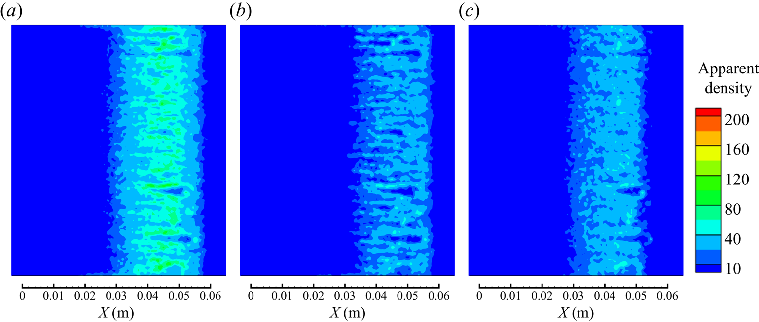
Figure 13. Instantaneous snapshots of the apparent density of particle phases at a normalized time  $\tilde {t}=193.0$: (a) the whole solid particle phases (summation of particles from phases 1 and phase 2), (b) the 1st particle phase with
  $d_1=110$
  $\mathrm {\mu }$m and (c) the 2nd particle phase with
  $d_2=120$
  $\mathrm {\mu }$m. Note that only the region of
  $[0\ \textrm {m}, 0.06\ \textrm {m}] \times [-0.04\ \textrm {m}, 0.04\ \textrm {m}]$ is shown here.
In the experiment, the solid particle curtain is generated by the free fall of particles from a reservoir into the test section (Ling et al. Reference Ling, Wagner, Beresh, Kearney and Balachandar2012). As pointed out in the experiment, the particle curtain occupies approximately 87 % in the spanwise direction ( $y$ direction in figure 11). Therefore, a gap between the particle curtain and the walls exists, which is studied here as well. According to the experiment with 87 % occupation by the particle curtain in the tube, a 13 % gap close to the wall will be taken into account. With the new set-up, the newly calculated pressure and particle trajectories are given in figure 14. Interestingly, the pressure variation at the downstream gauge position at time
  $\tilde {t}=50\unicode{x2013} 80$ has an early drop and a later increase in gas pressure after the passage of the transmitted shock and has a better agreement with the experimental data than the previous calculation with 100 % particle curtain occupation, which is marked by the blue circle in figure 14.
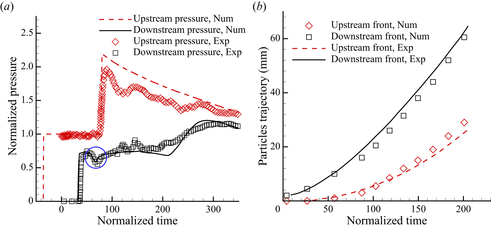
Figure 14. Numerical results (denoted by ‘Num’) and experimental measurements (denoted by ‘Exp’) with  $87\,\%$ spanwise particle occupation as shown figure 11(b): (a) the time-dependent gas pressure at upstream and downstream gauge points; (b) the trajectories of particle cloud fronts.
5. Conclusion
In this paper, a multiscale GKS-UGKWP method is developed for the polydisperse gas-particle system. Particularly, the cell resolution-dependent dynamic model for the system with a coupled disperse solid particle phase and gas phase is directly used in the design of the corresponding multiscale method. In order to capture both equilibrium and non-equilibrium particle evolution processes efficiently, the particle distribution function is decomposed into wave and discrete particle components in UGKWP according to the respective local Kn for each solid particle phase. The UGKWP will choose an optimal way to describe the dynamics of solid particles by separately evolving the Eulerian deterministic wave and tracking the individual Lagrangian particle with a balance of physical accuracy and numerical efficiency. The properties of the solid particles, such as the particle size, concentration and concrete material, have been taken into account in the determination of the solid particle dynamics. One distinguishable feature in UGKWP is that the wave–particle decomposition can automatically lead the scheme to the EE and EL methods for the gas–solid particle system in the corresponding equilibrium and non-equilibrium regimes for the solid particle phase. Two cases of dense polydisperse flow in the fluidization bed are studied. Specifically, in the FCC catalyst reactor, the diameters of large millet particles and small FCC catalyst particles differ in particle size by  $15$ times. The numerical experiments show that only the fine FCC catalyst particles appear in the top zone of the riser, while the millet particles only exist in the bottom dense region. In addition, for the FCC catalyst phase, the discrete particle description plays a key role in the top dilute regions, and the wave description contributes mostly in the bottom dense zone region, even with the existence of a tremendous number of real particles. For the large particle phase, millet particles only exist in the bottom dense region and need a discrete particle description to capture the local non-equilibrium state. The above observation indicates the flexibility of wave–particle decomposition in describing the disperse solid phases and the adaptivity in dynamically following the equilibrium and non-equilibrium flow evolutions. At the same time, the interaction of a
  $Ma=1.66$ shock wave impinging on a dense particle curtain with polydisperse solid particle phases is studied by the current method. The numerical solutions, such as the pressures of the gas flow at gauge points and the trajectories of the fronts of the solid particle cloud, are compared with the experimental measurements. Even though the current studies only involve the particle system with two dispersed phases, the algorithm itself can be easily extended to a gas-particle system with multiple dispersed solid particle phases. Overall, the decomposition of the wave and particle evolution for the solid particle phase has advantages in simulating the polydisperse gas-particle multiphase flows with a multiscale nature.
Funding
The current research is supported by National Key R&D Program of China (grant nos. 2022YFA1004500), National Science Foundation of China (12172316), and Hong Kong research grant council (16208021, 16301222).
Declaration of interests
The authors report no conflict of interest.
Appendix A. The mixed wall boundary condition for the solid particle phase
This section introduces the details of the mixed wall boundary condition for the solid particle phase employed in this paper. More specifically, the tangential velocity near the wall,  $v_{t}^*$, will be determined based on the method proposed by Johnson and Jackson (Johnson & Jackson Reference Johnson and Jackson1987). For the wall stress
 \begin{equation} \tau_w \overset{def}{=} \mu \frac{\partial v}{\partial x}= \frac{\rm \pi}{6} \sqrt{3\theta_s} \rho_s g_0 \frac{\epsilon_s}{\epsilon_{s,max}} \phi v_{slip}, \end{equation}
where  $v_{slip} = v_{t}^* - v_{wall}$ is the slip velocity between solid particles and the wall, and
  $v_{slip} = v_{t}^*$ for the fixed wall. With the introduction of
  $A$
$A$
 \begin{equation} A \overset{def}{=} \frac{\rm \pi}{6} \sqrt{3\theta_s} \rho_s g_0 \frac{\epsilon_s}{\epsilon_{s,max}} \phi v_{t}^*, \end{equation}
and the discretization of  ${\partial v}/{\partial x}$, (A1) can be written as
 \begin{equation} \mu \frac{v_{t,c} - v_{t}^*}{\Delta x / 2} = A v_{t}^*, \end{equation}
where  $v_{t,c}$ is the tangential velocity at the centre point of the near-wall cell. Therefore,
  $v_{t}^*$ can be determined as
 \begin{equation} v_{t}^* = B v_{t,c}, \quad B \overset{def}{=} \frac{1}{1 + A\Delta x /2\mu}, \end{equation}
where  $\phi \in [0,1]$ is the so-called specularity coefficient. In this paper,
  $\phi$ is evaluated by
  $\phi = ({\epsilon _s}/{\epsilon _{s,max}})^{\omega }$ with
  $\omega = 4$. Then, in the dilute region with small
  $\epsilon _s$,
  $\phi \to 0$, we have
  $A \to 0$,
  $B \to 1$,
  $v_{t}^* \to v_{t,c}$. The tangential velocity of the particle phase near the wall will be the same as that in the near-wall cell. On the contrary, in the dense region with large
  $\epsilon _s$ and
  $\phi$ (with the maximum value 1), we get
  $g_0 \to \infty$ ,
  $A \to \infty$,
  $B \to 0$,
  $v_{t}^* \to 0$. The tangential velocity of the particle phase near the wall approaches to 0.
In the simulation, the solid particle velocity at the inner side of the wall, denoted as  $(v^{l}_{t}, v^{l}_{n})$, can be obtained by reconstruction. Then, the solid particle velocity at the outer side of the wall, denoted as
  $(v^{r}_{t}, v^{r}_{n})$, can be obtained as the following:
 \begin{equation} v^{r}_{t} = (2B-1) v^{l}_{t},\quad v^{r}_{n} ={-}v^{l}_{n}. \end{equation}
Besides, the solid volume fraction and granular temperature at the outer side of the wall are assumed to be equal to the corresponding values at the inner side by reconstruction, which implies,  $\epsilon _s^{r} = \epsilon _s^{l}$ and
  $\theta _s^{r} = \theta _s^{l}$. As a result, the fluxes for solid particles at the wall can automatically accommodate the slip and no-slip wall boundary conditions in the limiting dilute and dense flows, respectively.


