1. Introduction
With the development of deep learning (DL), target detection algorithms have been applied in many fields and achieved state of the art results (LeCun et al., Reference LeCun, Bengio and Hinton2015). Meanwhile, the development of large survey telescopes, such as the Sloan Digital Sky Survey (SDSS; York et al. Reference York, Adelman and Anderson2000) allows easier access to astronomical image data. Accordingly, target detection algorithms can be applied to massive astronomical images to provide celestial body detection by using the morphological structure and colour information contained in the images. Moreover, faint object detection in astronomical images can be technically solved. Cataclysmic variables (CVs) are a class of short-period binaries consisting of an accreting white dwarf (WD) primary star and a low-mass main-sequence secondary star as the mass donor (Warner, Reference Warner2003). CVs can be classified into minor sub-types according to their amplitudes, timescale variability, and magnetism. CVs are also a class of periodic variables with complex spectral and orbital light curve variation (Hellier, Reference Hellier2001). CVs are a hot spot for astrophysical research due to their complex physical composition and variability, and are also a natural laboratory for studying accretion processes. Furthermore, CVs are the ideal objects for accretion observations than other objects with accretion processes because of their close distances.
According to theoretical calculations, the Milky Way should have about 10 million CVs, but only 1829 CVs have been documented to dateFootnote a , of which only 1600 have been confirmed (Downes & Shara, Reference Downes and Shara1993). This notion indicates the difficulty of discovering CVs and reflects the significance of searching for CVs.
Spectra can confirm CVs because they have strong emission lines, particularly during quiescence. Most optical spectra of CVs (Figure 1) show hydrogen Balmer emission lines, namely, 6563Å, 4862Å, 4341Å, 4102Å, and HeI 5876Å and HeII 4686Å during quiescence. Even conventional classification methods with prominent features can easily identify CVs from spectra. However, the number of spectra is limited due to the relatively high observation cost.

Figure 1. A CV spectrum from SDSS.
Photometric selection and brightness change is the most commonly used method in the search for CVs. CV candidates can be roughly selected out by photometric information and identified with spectra or follow-up observations. Wils et al. (2010) used the photometric selection criteria of
 $((u - g) + 0.85*(g - r) \lt 0.18)$
to search for dwarf novas. Szkody et al. (Reference Szkody, Anderson and Agüeros2002, Reference Szkody, Fraser and Silvestri2003, Reference Szkody, Henden and Fraser2004, Reference Szkody, Henden and Fraser2005, Reference Szkody, Henden and Agüeros2006, Reference Szkody, Henden and Mannikko2007, Reference Szkody, Anderson and Hayden2009) established a photometric selection criterion, i.e.
$((u - g) + 0.85*(g - r) \lt 0.18)$
to search for dwarf novas. Szkody et al. (Reference Szkody, Anderson and Agüeros2002, Reference Szkody, Fraser and Silvestri2003, Reference Szkody, Henden and Fraser2004, Reference Szkody, Henden and Fraser2005, Reference Szkody, Henden and Agüeros2006, Reference Szkody, Henden and Mannikko2007, Reference Szkody, Anderson and Hayden2009) established a photometric selection criterion, i.e.
 $(u - g \lt 0.45, g - r \lt 0.7, r - i \gt 0.3, i -z \gt 0.4)$
to select WD-main sequence binaries with a few CVs and confirmed 285 CVs. These criteria overlap with quasars, faint blue galaxies, and WDs. In essence, there is no authorised criterion for CVs which is available at present. Drake et al. (Reference Drake, Gänsicke and Djorgovski2014) obtained 855 candidates from the Catalina Real-Time Transient Survey (Drake et al. Reference Drake, Djorgovski and Mahabal2011) by using the transient detection procedure. Mroz et al. (Reference Mroz, Udalski and Poleski2016) received 1091 dwarf nova samples from the Optical Gravitational Lensing Experiment (Paczynski et al. Reference Paczynski, Stanek, Udalski, Szymanski and Preston1995) by using the Early Warning System (Udalski, Reference Udalski2004) and photometric curve analysis. Han et al. (Reference Han, Zhang and Shi2018) found three new candidates by cross-matching the catalogs of CVs with the Large Sky Area Multi-Object Fiber Spectroscopic Telescope (LAMOST; Cui et al. Reference Cui, Zhao and Chu2012) DR3.
$(u - g \lt 0.45, g - r \lt 0.7, r - i \gt 0.3, i -z \gt 0.4)$
to select WD-main sequence binaries with a few CVs and confirmed 285 CVs. These criteria overlap with quasars, faint blue galaxies, and WDs. In essence, there is no authorised criterion for CVs which is available at present. Drake et al. (Reference Drake, Gänsicke and Djorgovski2014) obtained 855 candidates from the Catalina Real-Time Transient Survey (Drake et al. Reference Drake, Djorgovski and Mahabal2011) by using the transient detection procedure. Mroz et al. (Reference Mroz, Udalski and Poleski2016) received 1091 dwarf nova samples from the Optical Gravitational Lensing Experiment (Paczynski et al. Reference Paczynski, Stanek, Udalski, Szymanski and Preston1995) by using the Early Warning System (Udalski, Reference Udalski2004) and photometric curve analysis. Han et al. (Reference Han, Zhang and Shi2018) found three new candidates by cross-matching the catalogs of CVs with the Large Sky Area Multi-Object Fiber Spectroscopic Telescope (LAMOST; Cui et al. Reference Cui, Zhao and Chu2012) DR3.
Traditional methods require a substantial amount of artificial time, sometimes years, to make follow-up observations. The manual techniques are not always accurate and frequently require many subjective judgements. With the simultaneous development of hardware and software in computer science, applying automated methods instead of manual methods can significantly increase efficiency and identification accuracy. Jiang & Luo (Reference Jiang and Luo2011) obtained 58 CV candidates in SDSS by using the algorithm of PCA+SVM with massive spectra produced by LAMOST and SDSS. Hou et al. (Reference Hou, Luo, Li and Qin2020) identified 58 new candidates by using bagging top push and random forest. Hu et al. (Reference Hu, Chen, Jiang and Wang2021) found 225 candidates by using the LightGBM algorithm and verified four new CV candidates. Considering the quantitative limitation of spectra, applying a detector that can automatically identify CVs in images is demanding.
You Only Look Once (YOLO) is an object detection method. Its latest framework, YOLOX (Ge et al., Reference Ge, Liu, Wang, Li and Sun2021) can achieve fast detection and excellent image processing performance. However, the pixels occupied by CVs are extremely limited in astronomical images, resulting in low-resolution problems, blurred and less information, shallow features (brightness and edge), and weak expressiveness. Accordingly, we improve YOLOX to achieve low-cost, fast, and accurate localisation and identification of CVs. We train and validate the model using SDSS images for detecting CVs.
This paper is organised as follows. Section 2 introduces the data. Section 3 briefly illustrates YOLOX and our improvements to the current framework. Section 4 describes the data preprocessing and image enhancement, the experimental procedure, the experimental environment, and the evaluation of the experimental results. Section 5 discusses the experimental results. A comparison with previous research methods is also presented. Section 6 provides the conclusions and a summary of the study.
2. Data
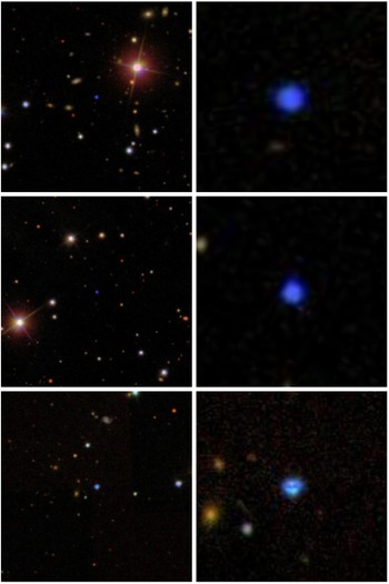
The SDSS (York et al. Reference York, Adelman and Anderson2000) provides a spectroscopic survey as well as a photometrically and astrometrically calibrated digital imaging survey. The photometric imaging includes five bands, namely, u, g, r, i, and z at the average wavelengths of 3551, 4686, 6165, 7481, and 8931Å, respectively. CVs are usually quite blue and faint objects. Our CV sample comes from Szkody et al. (Reference Szkody, Anderson and Agüeros2002, Reference Szkody, Fraser and Silvestri2003, Reference Szkody, Henden and Fraser2004, Reference Szkody, Henden and Fraser2005, Reference Szkody, Henden and Agüeros2006, Reference Szkody, Henden and Mannikko2007, Reference Szkody, Anderson and Hayden2009), and duplicate CVs are deleted. We have uploaded the images of CVs to GitHubFootnote b for viewing. Appendix A displays the existing CV photometric data with spectra. We construct the CV sample with SDSS images already synthesised with i, r, and g-bands corresponding to the R, G, and B channels to more wildly apply our method. The images of CV samples have a size of 0.39612"/pix, some of which are shown in Figure 2.

Figure 2. Some images from SDSS and CVs are at centre.
2.1. Image preprocessing and data augmentation
First, the images are cleaned, the noise in the images are filtered, and a small amount of noisy images are removed, and 208 images are obtained, while can remove the interference of background noise to a certain extent. Given the small number of samples, the data set needs to be expanded using data enhancement methods, which not only guarantee the diversity of the data set but also improve the detection performance and enhances the robustness and generalisation ability of the model. Our method of using data augmentation is to generate a rotation angle within every 30 degrees randomly, rotate the image counterclockwise, and then randomly shift and crop respectively, and the ranges of shifting and cropping are shown in Table 1. We use the Lanczos interpolation (Thevenaz & Blu, Reference Thevenaz and Blu2000) to avoid voids on the image. Lanczos interpolation has the advantages of fast speed, good effect, and the most cost-effective. The methods of translation and clipping can enhance the position of the target, and the method of rotation can significantly change the orientation of the object without adding topological information.
Table 1. Randomly shifting and cropping range.

tLeft, tRight, tTop, tBottom: the left, right, top, and bottom coordinates of the target in the image iWidth, iHeight: the width and height of the image
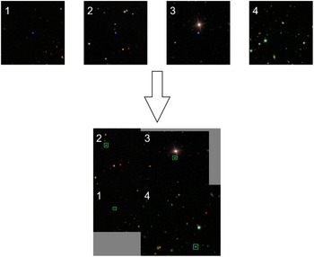
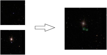
In the YOLOX model training stage, the algorithm will also randomly enhance the data, the usual methods are Mosaic (Bochkovskiy et al., Reference Bochkovskiy, Wang and Liao2020) and Mixup (Zhang et al., Reference Zhang, Cisse, Dauphin and Lopez-Paz2017), Mosaic first randomly selects four images for conventional enhancement, and then stitches them into a new image, so that the new image contains the random target box information of the extracted image, and the random method maximises the rich data set. Mosaic enhances the diversity of data, enriches the background of the image, and also increases the number of targets, and the four images stitched together into the network improve the batch size, and the mean and variance can be better calculated when performing BN operations. A mosaic example is shown in Figure 3. The core idea of Mixup is to randomly select two images from each batch and superimpose a certain proportion to generate new images, reducing the memory of the model on the noisy samples, thereby reducing the impact of noisy samples on the model. A mixup example is shown in Figure 4.

Figure 3. Data enhancement example by mosaic. Due to different size of each image, the blank is filled with grey colour when performing mosaic.

Figure 4. Data enhancement example by mixup.
2.2. Dataset
The external rectangular boxes of CVs in the image are drawn using the data set annotation software to achieve manual annotation of CVs, ensuring that the rectangular boxes contain as little background as possible in the process. The annotated information is saved as XML format files and converted into TXT text by the program, while facilitates the data reading by the model.
After the data enhancement operation, a total number of 5200 images are achieved. From these images, 60% of images are randomly selected as training set, 20% as validation set, and the rest as test set. Finally, the dataset is made into Pascal VOC style. The training set is used to train the model (i.e., to determine the model weights and biases for these parameters). The validation set is only for selecting hyperparameters, such as the number of network layers, the number of network nodes, the number of iterations, and the learning rate. The test set is used to evaluate the final model after the training is completed.

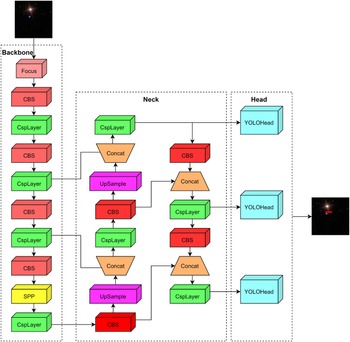
Figure 5. The architecture of YOLOX.
3. Method
The definition of small targets in Computer Vision is as follows (Chen et al., Reference Chen, Liu, Tuzel and Xiao2016): the median ratio of the target of the same category relative to the whole image area is between 0.08% and 0.58%. The most common definition is from the MS COCO (Lin et al., Reference Lin, Maire, Belongie, Hays and Zitnick2014) dataset, which defines a small target as a resolution of fewer than 32
 $\times$
32 pixels. According to the International Society for Optical Engineering definition, an imaging area of fewer than 80 pixels in a 256
$\times$
32 pixels. According to the International Society for Optical Engineering definition, an imaging area of fewer than 80 pixels in a 256
 $\times$
256 image is a small target. CV detection can thus be considered a detection task for small targets. Small targets contain little information, making it challenging to extract discriminative features. Existing DL methods for small target detection include multi-scale learning, contextual learning, adding attention mechanisms, generating super-resolution feature representations, anchorless mechanisms, and optimising loss-type handling disparity datasets. YOLO uses an end-to-end neural network that makes predictions of bounding boxes and class probabilities appropriate for CV detection. YOLOX is an anchor-free version of YOLO, with a more straightforward design but better performance. The attention mechanism allows the network to focus on what needs more attention. Adding the attention module to YOLO can effectively enhance the network’s ability to capture the image’s features. Convolutional Block Attention Module (CBAM; Woo et al. Reference Woo, Park, Lee and Kweon2018) is a simple and effective attention module for feedforward convolutional neural networks because of its lightweight and versatility and can be seamlessly integrated into YOLOX. The following introduces YOLOX and CBAM in detail. Inspired from these directions, we propose an improved CV object detection model.
$\times$
256 image is a small target. CV detection can thus be considered a detection task for small targets. Small targets contain little information, making it challenging to extract discriminative features. Existing DL methods for small target detection include multi-scale learning, contextual learning, adding attention mechanisms, generating super-resolution feature representations, anchorless mechanisms, and optimising loss-type handling disparity datasets. YOLO uses an end-to-end neural network that makes predictions of bounding boxes and class probabilities appropriate for CV detection. YOLOX is an anchor-free version of YOLO, with a more straightforward design but better performance. The attention mechanism allows the network to focus on what needs more attention. Adding the attention module to YOLO can effectively enhance the network’s ability to capture the image’s features. Convolutional Block Attention Module (CBAM; Woo et al. Reference Woo, Park, Lee and Kweon2018) is a simple and effective attention module for feedforward convolutional neural networks because of its lightweight and versatility and can be seamlessly integrated into YOLOX. The following introduces YOLOX and CBAM in detail. Inspired from these directions, we propose an improved CV object detection model.
3.1. YOLOX
YOLOX uses CSPDarkNet (Bochkovskiy et al., Reference Bochkovskiy, Wang and Liao2020) as the backbone following the filter size and overall structure of DarkNet (Redmon & Farhadi, Reference Redmon and Farhadi2017), adding a cross-stage partial structure to each residual block (He et al., Reference He, Zhang, Ren and Sun2016). Figure 5 shows the architecture of YOLOX.
YOLOX is a network composed of a feature pyramid network (FPN; (FPN; Deng et al. Reference Deng, Wang, Liu, Liu and Jiang2022) with a pixel aggregation network (PAN; (PAN;Wang et al. Reference Wang, Xie and Li2022), which is a fusion of high-level features by upsampling and low-level features to obtain a new feature map. Meanwhile, PAN fuses low-level features by downsampling and containing features further to pass up the robust localisation features. The final following feature maps of multi-scale features are obtained, which are used to detect large, medium, and small targets. YOLOX feeds the enhanced feature map into the head network for classification and localisation. Unlike the previous versions of YOLOX, YOLOX uses a decoupled head structure. The head structure is divided into two parts, namely, classification and localisation, which are separately implemented and then integrated into the final prediction stage. YOLOX proposes the SimOTA technique to dynamically match positive samples for targets of different sizes. The loss function of the YOLOX algorithm typically includes target, classification, and regression losses. Binary cross-entropy and IOU loss are used in target classification and regression separately. Classification and regression loss calculates the loss of positive samples. Meanwhile, target loss calculates the loss of positive and negative samples.

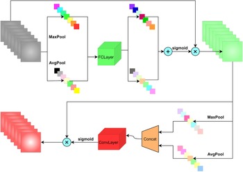
Figure 6. The basic structure and processing flow chart of CBAM.
3.2. CBAM
CBAM is a simple and effective attention module for feed-forward convolutional neural networks. This module processes the input feature map, derives the attention map along two separate dimensions, channel and space, and applies the result into the input feature map. The channel attention mechanism (CAM) uses parallel AvgPool and MaxPool approaches to process the input. The parallel connection approach loses less information than a single pooling; hence, this approach has more symbolic power. The CAM in CBAM differs from SEnet by adding a parallel max-pooling layer, which extracts more comprehensive and richer high-level features. The spatial attention mechanism (SAM) also uses parallel AvgPool and MaxPool approaches. Unlike CAM which sums two 1D attention data, SAM uses a convolutional approach to dimensionally compress the attention graph, which more effectively preserves the spatial information in the feature graph. Finally, CBAM combines the two modules, CAM and SAM, in a serial sequential way according to the ablation experiment.
The CBAM module can be inserted into YOLOX and helps the fusion of multi-scale features, by reducing the weights, and CBAM filters the factor that is detrimental to the model’s recognition ability, thus improving the network’s performance with only a small additional computational cost. Figure 6 shows the processing flow chart of CBAM.
3.3. Improved method
To make the YOLOX more suitable for identifying and localising CVs in images, we apply the following improvements: 1) The attention module of CBAM is adopted to direct the network’s attention on the important information of the target. 2) The number of output feature maps of the backbone is adjusted for small targets, adding a shallow feature map and inputting four feature maps into the improved FPN+PAN network for fusion. 3) Considering the overlap area, centroid distance, and aspect ratio between the prediction result and the actual target box, the CIOU (Zheng et al., Reference Zheng, Wang and Ren2021) loss for the regression loss is adopted. Accordingly, problems, such as performance degradation of YOLOX, are also addressed.
Specifically, we use CBAM to combine the channel and SAMs. Each channel can be considered a feature detector for the feature map. The CAM compresses the feature map in the spatial dimension to obtain a thought vector and then process it. The CAM focuses on what is essential in this image, and the mean pooling has feedback for each pixel point on the feature map. Although maximum pooling has feedback for gradients when performing gradient backpropagation, only the places in the feature map with the most significant response have feedback for gradients. The SAM is more concerned with where the essential parts are, and it compresses the channel dimension of the feature map to ensure that a two-channel feature map can be obtained for subsequent processing. The CBAM attention mechanism is a simple and effective attention module for feedforward convolutional neural networks because of its lightweight and versatility and can be seamlessly integrated into any network. The CBAM module can be inserted into YOLOX networks to more effectively mine CV features carried in astronomical images, which helps the fusion of multi-scale features, thus improving the performance of the network with a small additional computational cost.

Figure 7. The proposed pipeline.
In the convolutional neural network, the fewer the convolution operations, the lower the output feature map, the smaller the receptive field, the higher resolution of the feature map and the smaller the target features are retained. Using low-level feature maps is beneficial to the detection efficiency of small objects. We increase the number of output feature maps of the backbone network, add the feature maps after the 10th layer convolution operation to the output results, and enter the four feature maps into the improved FPN+PAN network for multi-scale feature fusion to ensure that the final fusion of three. This new feature map contains more small target features. Although the calculation amount of the fusion process increases, it is beneficial to the future identification and positioning of CVs.
 \begin{equation}IOU=\frac{intersection}{union}.\end{equation}
The loss function makes the detection more accurate and localisation more precise, reflecting the error between the prediction result of the detection algorithm and the actual target. IOU loss (Yu et al., Reference Yu, Jiang, Wang, Cao and Huang2016) is normally used in the regression to measure the degree of overlap. In Formula 1, this factor can efficiently respond to the degree of overlap and provide a scale without deformation. We use CIOU loss as the regression loss, considering the overlap area, centroid distance, and aspect ratio to more stably optimise the model. The model can more accurately locate CVs, and its calculation is shown in Formulas 2, 3, and 4, where b and
 $b^{gt}$
denote the centre coordinates of the prediction and true boxes respectively; d denotes the Euclidean distance between the centre coordinates of the prediction and true boxes; c denotes the diagonal distance of the minimum external matrix of the prediction and true boxes; w and
$b^{gt}$
denote the centre coordinates of the prediction and true boxes respectively; d denotes the Euclidean distance between the centre coordinates of the prediction and true boxes; c denotes the diagonal distance of the minimum external matrix of the prediction and true boxes; w and
 $w^{gt}$
denote the width of the prediction and true boxes, respectively; and h and
$w^{gt}$
denote the width of the prediction and true boxes, respectively; and h and
 $h^{gt}$
denote the height of the prediction and true boxes, respectively.
$h^{gt}$
denote the height of the prediction and true boxes, respectively.
 \begin{equation} CIOU=IOU-\frac{\rho^2(b,b^{gt})}{c^2}-\alpha v,\end{equation}
 \begin{equation} \alpha = \frac{v}{(1-IOU)+v},\end{equation}
 \begin{equation} v=\frac{4}{\pi^2}\left(arctan\frac{w^{gt}}{h^{gt}}-arctan\frac{w}{h}\right)^2.\end{equation}
Table 2. Results of ablation experiments.

Table 3. Comparison of mAP, Precision, Recall, and
 $F1-Score$
of our improved YOLOX model with the original YOLOX model and LightGBM.
$F1-Score$
of our improved YOLOX model with the original YOLOX model and LightGBM.

Table 4. Model speed evaluation for 10 times.

4. Experiment
The flowchart of the whole procedure is shown in Figure 7. The preparation for annotating images and data enhancement is introduced in Section 4.1, and this step is required during the training model phase. The environment is set up before conducting the experiments in Section 4.5. Afterwards, we use the improved model to obtain prediction results. In the training model phase, the model parameters need to be improved based on the resulting deviations. In the test phase, the results are used to evaluate the effectiveness of the model using the evaluation criteria adopted in Section 4.2. In the prediction phase, the prediction target boxes are drawn based on the results. Ablation experiments in Section 4.3 are performed to verify the effectiveness of each improved model based on the training and test results.
4.1. Evaluation index
We use Mean Average Precision (mAP; (mAP; Everingham et al. Reference Everingham, Eslami and Van Gool2015), Precision, Recall, and
 $F1-Score$
as experimental metrics. Precision is the proportion of correct results among all predicted targets. Meanwhile, Recall is the proportion of correct results relative to all true targets. The calculation methods are shown in Formulas 5 and 6, where TP is the number of predicted bounding boxes with IOUs greater than the threshold value, FP is the number of predicted bounding boxes with IOUs less than or equal to the threshold value, and FN is the number of predicted bounding boxes that do not match the true target box. Setting different thresholds can result in distinct (P, R) values, refracting the (P, R) values corresponding to different thresholds on a 2D coordinate system and connecting them into a curve. The mAP is the average of AP of each category, and AP is the area under the P-R curve. As shown in Formula 7,
$F1-Score$
as experimental metrics. Precision is the proportion of correct results among all predicted targets. Meanwhile, Recall is the proportion of correct results relative to all true targets. The calculation methods are shown in Formulas 5 and 6, where TP is the number of predicted bounding boxes with IOUs greater than the threshold value, FP is the number of predicted bounding boxes with IOUs less than or equal to the threshold value, and FN is the number of predicted bounding boxes that do not match the true target box. Setting different thresholds can result in distinct (P, R) values, refracting the (P, R) values corresponding to different thresholds on a 2D coordinate system and connecting them into a curve. The mAP is the average of AP of each category, and AP is the area under the P-R curve. As shown in Formula 7,
 $F1-Score$
is the summed average of Precision and Recall.
$F1-Score$
is the summed average of Precision and Recall.
In target detection, mAP is the most convincing evaluation index. We use the YOLO algorithm corresponding to the [email protected] and mAP [0.5:0.95] to evaluate our model. [email protected] is the average of all categories of AP and mAP [0.5:0.95] is to set the IOU thresholds as 0.5, 0.55, 0.6, 0.65, 0.7, 0.75, 0.8, 0.9, and 0.95 when averaged. The higher mAP of a model, the better the corresponding detection will be.
 \begin{equation}Precision=\frac{TP}{TP+FP},\end{equation}
 \begin{equation}\ \ \ Recall=\frac{TP}{TP+FN},\end{equation}
 \begin{equation}\ \ \ F1-{}Score=2 \times \frac{Precision \times Recall}{Precision+Recall}.\end{equation}
In order to reflect the fast speed of the model, the common indicator for evaluating speed in object detection is frame rate per second (FPS), that is, the target network can process the number of pictures per second, FPS is simply understood as the refresh rate of the image, that is, how many frames per second, assuming that the target detection network processes 1 frame to 0.02 s, at this time FPS is 1/0.02 = 50. We train the model in the same hardware environment that evaluates the monitoring speed using the time it takes to process an image. The shorter the time, the faster the speed is.
4.2. Ablation study
We apply three modules to improve YOLOX for small target detection. The three modules can be summarised as adding CBAM, adding feature maps to FPN+PAN, and adjusting the regression loss to CIOU. We perform an ablation study on the model to verify the contribution of the three modules to the detection improvement, and all experimental data sets and hyperparameter configurations are the same as before. Table 2 shows the experimental results. In comparison with the original YOLOX, mAP is improved by adding NFPAN module or CIOU module. Meanwhile, mAP is decreased by only adding CBAM module. However, the results from adding CBAM and CIOU modules show that CBAM is effective based on CIOU. According to the results of the three groups with adding the two modules, CIOU is more significant to improve the performance than NFPAN or CBAM. Considering all the three modules, the performance of the model is the best. Therefore the improvement of our model is effective in identifying CVs.
4.3. Experimental results
We compare the performance of the YOLOX models with the classification model of Hu et al. (Reference Hu, Chen, Jiang and Wang2021) using the LightGBM algorithm. The mAP, Precision, Recall, and
 $F1-Score$
of the three models are shown in Table 3. Hu et al. (Reference Hu, Chen, Jiang and Wang2021) used LightGBM from the LAMOST-DR7 spectra to automatically search for CV candidates, which extracts the potential relationships concerning CV spectra. LightGBM combines multiple features to prevent the interference of individual features by noise and finally achieves 95.21% Precision, 93.53% Recall, and 94.36%
$F1-Score$
of the three models are shown in Table 3. Hu et al. (Reference Hu, Chen, Jiang and Wang2021) used LightGBM from the LAMOST-DR7 spectra to automatically search for CV candidates, which extracts the potential relationships concerning CV spectra. LightGBM combines multiple features to prevent the interference of individual features by noise and finally achieves 95.21% Precision, 93.53% Recall, and 94.36%
 $F1-Score$
. The model’s classification performance is excellent because spectra contain more abundant information than images, and the data processing is fast due to the small model. LightGBM is a classification model that only works with spectra. The YOLOX models can achieve CV recognition and localisation in astronomical images, especially the improved YOLOX model with 92.9% Precision, 94.3% Recall, and 93.6%
$F1-Score$
. The model’s classification performance is excellent because spectra contain more abundant information than images, and the data processing is fast due to the small model. LightGBM is a classification model that only works with spectra. The YOLOX models can achieve CV recognition and localisation in astronomical images, especially the improved YOLOX model with 92.9% Precision, 94.3% Recall, and 93.6%
 $F1-Score$
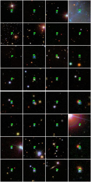
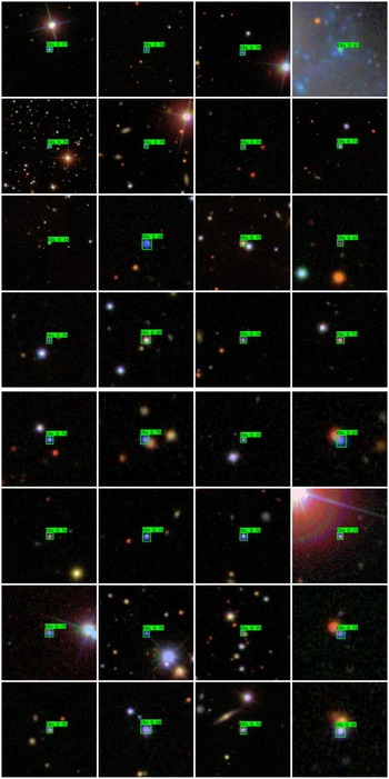
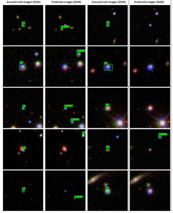
. The target detection algorithm is to classify and regress each pixel point on the extracted feature map. Accordingly, the task of the target detection model will be more complicated than the classification model, and the accuracy will be reduced only based on images. Nonetheless, the target detection algorithm will be more advantageous for massive astronomical images when spectral observation is expensive. Figures 8 and 9 show the effect of the detection of CVs in the images. The cases where the predicted results differ from the ground truth are shown in Table 5.
$F1-Score$
. The target detection algorithm is to classify and regress each pixel point on the extracted feature map. Accordingly, the task of the target detection model will be more complicated than the classification model, and the accuracy will be reduced only based on images. Nonetheless, the target detection algorithm will be more advantageous for massive astronomical images when spectral observation is expensive. Figures 8 and 9 show the effect of the detection of CVs in the images. The cases where the predicted results differ from the ground truth are shown in Table 5.
To evaluate the deviation of the results detected by our model from the actual results, we calculate the pixel distance between the predicted results of the model and the centre of the actual target on the test set, because we use an image of 0.39612"/pix, and the final result of the experiment is that the centre mean arcsecond deviation is 0.8058".

Figure 8. Ground truth of the image samples from SDSS.

Figure 9. Predicted image samples from SDSS.
We select an image from the dataset to evaluate the speed of the model. We test it for 10 times under the same hardware conditions to calculate the FPS, and the results are shown in Table 4. The final result averages them, and the FPS of our model is 30.9165.
Table 5. The cases where the predicted results differ from the ground truth.

4.4. Experimental environment
Tables 6 and 7 show the software and hardware environment of the experiment and the hyperparameters used for model training. Given that we use 16 samples as a batch size when training the model and the network’s depth is deep, we use NVIDIA GeForce RTX 3070 for acceleration. Furthermore, PyTorch calls to take advantage of a complete graphics card for complex parallel computing. In the training stage, the frozen training method can speed up the efficiency of model training and prevent the weights from being destroyed. In the freezing stage, the backbone network of the model is frozen, the parameters of the feature extraction network do not change, and the memory usage is negligible. In this stage, only the network is fine-tuned. In the thawing stage, the backbone network of the model is not frozen, and all competitions in the network will change, occupying a large amount of GPU memory.
5. Discussion
The experimental results illustrate that the improved CV detection model can effectively localise and classify CVs in images. In the face of massive astronomical images, our model takes shorter time with satisfactory accuracy, which is crucial for fully using the observation data produced by large survey telescopes.
Considering the vast amount of astronomical images, we choose the fast and accurate YOLOX target detection algorithm to achieve the localisation and recognition of astronomical images. To address the problem that the DL algorithm degrades in accuracy when facing small targets, YOLOX is improved by adding an attention mechanism, adjusting the backbone output and the FPN+PAN network structure, switching to a suitable loss function, and applying data enhancement methods according to the characteristics of astronomical images. These improvements enhance the adaptability and effectiveness of the model for the CV detection task.
For existing supervised learning methods, the images of the corresponding objects must be recollected to train the model when identifying and locating other types of objects. Most DL algorithms lose accuracy when faced with small targets. Our model needs further improvement to cope up with this degradation to improve accuracy.
The YOLOX target detection model can localise and identify all CVs in the image and complete the detection of all targets. However, our model only tests the case with one CV in the image because each astronomical image we download contains only one object. In the future, we will further investigate scenes with multiple targets in the image. Our method will be improved by further optimising the loss function and neural network architecture to enhance our model’s classification and localisation performance for small target objects. We will also enhance the model’s performance by considering the background of CVs in astronomical images and extracting rich available features. In addition, different types of astronomical objects will be extended to increase the amount of data available to us.
Table 6. Experimental environment.

Table 7. Hyperparameters of the improved YOLOX model.

Accordingly, the improved models can locate, detect, and classify CVs simultaneously and are easy to encapsulate into the software. We will further strengthen the learning ability of the network by combining other observed CV data (e.g., spectroscopic and infrared data) with image data for analysis. When processing astronomical data, we will also consider cross-matching data from different astronomical telescopes and fusing the features of other data to improve the accuracy of our model. Another exciting improvement direction is to fully use the fast target detection function of YOLOX to achieve classification and localisation of CVs from images generated by ordinary telescopes. We will also consider how to better exploit our model’s localisation property in astronomical image recognition.
6. Conclusions
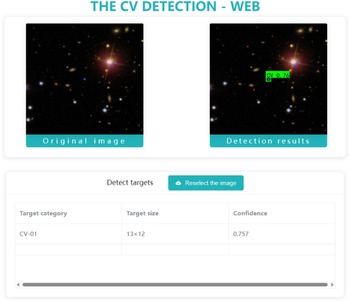
We propose an improved CV detector based on the YOLOX framework for the automatic identification and localisation of CVs to take advantage of astronomical images conveniently. This tool is helpful for the discovery of CVs, for the subsequent study of their physical composition and change mechanisms, and research on the accretion process in astrophysics. For the characteristics of astronomical optical images, we improve YOLOX by adding an attention mechanism and backbone output feature maps to make the fused features more multi-scale, adjusting the appropriate loss function, and adopting data enhancement. The experiments prove that the improved model performs better than the original YOLOX and demonstrate our model’s accuracy and robustness for processing optical images observed by astronomical telescopes to identify and localise CVs in the images. The actual use of test sets to judge the model confirms that the performance of the improved model is superior to that of the original algorithm, and the improved model has higher accuracy and robustness while ensuring detection speed. This mechanism will further facilitate astronomers’ research and improve the accuracy of models and the reliability of judgments. The relevant toolkit is under development. We used Flask+Vue for rapid modern web application development, and built a simple user interface of CV detection toolkit, shown in Figures B1 and B2 in Appendix B. This toolkit will make our research more accessible for astronomers, and we hope to see more exciting and new discoveries of CVs or other kinds of celestial objects by means of it.
Acknowledgements
We thank the referee very much for his valuable suggestions and comments. This paper is funded by the National Natural Science Foundation of China (Grant Nos. 12273076, 12133001 and 11873066), the Science Research Grants from the China Manned Space Project (Nos. CMS-CSST-2021-A04 and CMS-CSST-2021-A06), and Natural Science Foundation of Hebei Province (No. A2018106014). Funding for the Sloan Digital Sky Survey IV has been provided by the Alfred P. Sloan Foundation, the U.S. Department of Energy Office of Science, and the Participating Institutions. SDSS-IV acknowledges support and resources from the Center for High-Performance Computing at the University of Utah. The SDSS website is www.sdss.org. SDSS-IV is managed by the Astrophysical Research Consortium for the Participating Institutions of the SDSS Collaboration including the Brazilian Participation Group, the Carnegie Institution for Science, Carnegie Mellon University, the Chilean Participation Group, the French Participation Group, Harvard-Smithsonian Center for Astrophysics, Instituto de Astrofísica de Canarias, The Johns Hopkins University, Kavli Institute for the Physics and Mathematics of the Universe (IPMU) /University of Tokyo, Lawrence Berkeley National Laboratory, Leibniz Institut für Astrophysik Potsdam (AIP), Max-Planck-Institut für Astronomie (MPIA Heidelberg), Max-Planck-Institut für Astrophysik (MPA Garching), Max-Planck-Institut für Extraterrestrische Physik (MPE), National Astronomical Observatories of China, New Mexico State University, New York University, University of Notre Dame, Observatário Nacional/MCTI, The Ohio State University, Pennsylvania State University, Shanghai Astronomical Observatory, United Kingdom Participation Group, Universidad Nacional Autónoma de México, University of Arizona, University of Colorado Boulder, University of Oxford, University of Portsmouth, University of Utah, University of Virginia, University of Washington, University of Wisconsin, Vanderbilt University, and Yale University.
Data availability
This article’s data are available in SDSS, at http://cas.sdss.org/dr7/en/.
Appendix A. The CV photometric data

Appendix B. The CV detection toolkit

Figure B1. The user interface of CV detection toolkit.

Figure B2. The detected result display of an upload image by the trained improved YOLOX model.