


1. Introduction
Envisage the airflow around the wing of a commercial aircraft in a flight condition where the wing surface is covered with a thin water film that may be formed due to the de-icing process or while the aircraft encounters high liquid clouds particularly in the ascent and descent phases of flight. We conducted linear stability analysis and found that the boundary layer over a flat plate that is covered by a liquid film is receptive to the wall vibrations. The full linear stability analysis of multi-fluid flows is presented in Khoshsepehr (Reference Khoshsepehr2020, pp. 11–56). Now to predict the position of laminar–turbulent transition of the flow past the wing, we perform the linear receptivity analysis which is concerned with the first stage of the transition; that is, concerned with process of the external disturbances such as wall vibrations transforming into the instability modes in the form of Tollmien–Schlichting waves. Receptivity theory is one of the well-studied topics in fluid mechanics and it has been inspected by many researchers. Initially it was Lin (Reference Lin1946) who developed the triple-deck model in context of linear stability analysis of the boundary layer. The studies by Neiland (Reference Neiland1969) and Stewartson & Williams (Reference Stewartson and Williams1969) are the first theoretical analyses that describe the separation phenomena of a steady supersonic boundary layer using a triple-deck structure. Stewartson (Reference Stewartson1969) and Messiter (Reference Messiter1970) took the same approach to examine the incompressible flow near the trailing edge of a flat plate. Eventually it was Smith (Reference Smith1979) who verified the formulation of the triple-deck model to describe the instability modes of the boundary later.
Receptivity theory is an advanced theoretical method in fluid dynamics, employed by many authors to study different types of high-speed flows. However, transonic flows and especially multi-fluid flows have not received much attention. Hence, we investigate the stability analysis of a transonic boundary layer over a vibrating wall coated with a thin liquid film. Analyses presented in this paper are based on the triple-deck structure that describes the interaction of viscous and inviscid parts of the airflow. This structure is composed of (i) the near-wall nonlinear viscous sublayer with thickness  $O(Re^{-5/8})$ which occupies an
  $O(Re^{-1/8})$ portion of the boundary layer. The flow velocity in this tier is relatively slow, hence it is very sensitive to pressure variations. Even a slight raise in the pressure could lead to growth of the airflow filaments and alteration of the streamlines due to the significant deceleration of fluid particle in this tier. The slope of the streamlines is transmitted through (ii) the main part of the boundary layer with
  $O(Re^{-1/2})$. This middle tier has no contributions to the streamline displacement and merely acts as a transmitter between the viscous sublayer and (iii) the potential flow region situated outside the boundary layer with
  $O(Re^{-3/8})$. The latter tier is able to convert the slope perturbations into the pressure perturbations. Then these perturbations are transmitted back through the middle tier (boundary layer) to the viscous sublayer, intensifying the process of fluid deceleration. Assuming the film thickness is the same order quantity of the viscous sublayer, we derive a set of governing equations and appropriate boundary and interfacial conditions for the film flow. Consequently, the pressure perturbations produced and transmitted to the viscous sublayer by the film is considered in the hierarchical structure. As we assume the vertical dimension of the film is much smaller than the horizontal dimension, the lubrication theory is valid and the so-called lubrication equations describe the film flow.
To develop our model, we focus on the theory proposed by Timoshin (Reference Timoshin1990) that is devoted to transonic boundary-layer receptivity analysis of flows to external disturbances. This work is concerned with asymptotic description of instability modes in transonic flow, and we shall adopt a similar approach to find the quantity order of the free-stream Mach number. We extend the description of the transonic flow suggested by Timoshin (Reference Timoshin1990) to a multi-fluid flow where the flow encounters a subsonic and then a transonic free-stream flows. Specifically, we formulate the interaction problem to drive the affine transformation variables for both air and film flows. Then we match these variables with the estimates for fluid dynamic quantities of the unsteady potential equation in the free-stream flow, as the unsteady Kàrmàn–Guderley equation is recovered. This leads to realisations that the compressibility parameter in transonic flow becomes  $O(\sigma _{\mu }^{4/9} Re^{-1/18})$ and the time scale is
  $O(Re^{-2/9} \sigma ^{-11/9})$. Consequently, we present the description for the three tiers of the airflow and of the film flow in the interaction region. We display the receptivity coefficient to the vibrating wall perturbations by deriving the amplitude of the Tollmien–Schlichting waves in analytic form.
Another early study of the transonic boundary-layer transition by employing the viscous–inviscid interaction was conducted by Bowles & Smith (Reference Bowles and Smith1993). For a review on the generation of the Tollmien–Schlichting wave provoked by wing vibrations see Ruban, Bernots & Pryce (Reference Ruban, Bernots and Pryce2013). In addition, an extensive description of transonic flows is presented in Ruban (Reference Ruban2015). He focused on shock waves and separation analysis of transonic flows where the flows are treated as irrotational. As most commercial aircraft travel at transonic speed and transonic flows have immense practical importance to the aerospace industry; these flows are well investigated in the context of separation and shock waves. However, the receptivity of multi-fluid flows and surface tension effects have not been fully studied. In this work we diagnose such flows. In the following study we advance the analysis of an unsteady two-dimensional transonic flow by developing a triple-deck model that describes the instability waves. These waves appear as the first stage of the laminar–turbulent transition begins to unfold. A more recent study on transonic flow was presented by Ruban, Bernots & Kravtsova (Reference Ruban, Bernots and Kravtsova2016), who focused on linear and nonlinear receptivity analyses of the flow to a weak acoustic noise with an assumption that there is a small roughness on the wall surface. They also analysed the effect of flow separation on transition to turbulence. They found that the flow separation leads to a significant enhancement of the receptivity process.
In the next section we formulate a problem which enables us to find the receptivity coefficient for compressible boundary layer to a vibrating wall where the Mach number is close to one. The frequency of the vibration is chosen to be  $\omega =O(\sigma _{\mu }^{11/9} Re^{4/18})$ and the length of the vibration section
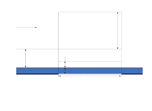
  $\Delta x=O(\sigma _{\mu }^{-1/3}Re^{-1/3})$, these scalings ensure that the triple-deck model is valid for the transonic flow. Then we assess the effect of film surface tension and its initial thickness as Kàrmàn–Guderley parameter varies. Figure 1 displays a schematic of the transonic flow regimes. We start the next section by showing how the incompressible flow theory may be extended to subsonic flow as the Mach number
  $M_{\infty }$ approaches one.

Figure 1. Schematic comparison of different flow regimes.
2. Problem formulation
Let us consider a perfect gas flow past a flat plate coated with a liquid film. We assume that the plate is aligned with the velocity vector in the oncoming flow. We further assume that the flat plate is vibrating periodically in time. Our task is to study the interaction of these wall vibrations with a small roughness on the plate surface at distance  $L$ from the leading edge. To study a two-dimensional flow we use the Cartesian coordinates
  $(\hat {x}, \hat {y})$, with
  $\hat {x}$ measured along the flat plate surface from its leading edge
  $O$ and
  $\hat {y}$ in the perpendicular direction. The velocity components in these coordinates are denoted by
  $(\hat {u} , \hat {v})$. We denote time, gas density, pressure, enthalpy and dynamic viscosity coefficient by
  $\hat {t}$,
  $\hat {\rho }$,
  $\hat {p}$,
  $\hat {h}$ and
  $\hat {\mu }$, respectively. The non-dimensional variables in the airflow are introduced as
 \begin{equation} \left.\begin{gathered} \hat{t} = \frac{L}{V_{\infty }} t ,\quad \hat{x} = L x ,\quad \hat{y} = L y ,\\ \hat{u} = V_{\infty } u , \quad \hat{v} = V_{\infty } v, \quad \hat{\rho } = \rho _{\infty } \rho ,\\ \hat{p} = p_{\infty } + \rho _{\infty } V_{\infty }^2 p , \quad \hat{h} = V_{\infty }^2 h, \quad \hat{\mu } = \mu _{\infty } \mu , \end{gathered}\right\} \end{equation}
with  $V_{\infty }$,
  $p_{\infty }$,
  $\rho _{\infty }$ and
  $\mu _{\infty }$ being the dimensional free-stream velocity, pressure, density and viscosity, respectively. The ‘hat’ is used here for dimensional variables and ‘prime’ for physical quantities in the film flow. The non-dimensional variable for the interface shape is defined as
 \begin{equation} \hat{H}= L H. \end{equation}
In the non-dimensional variables, the Navier–Stokes equations are written as
 $$\begin{gather}
\rho \left(\frac{\partial u}{\partial t} + u \frac{\partial
u}{\partial x} + v \frac{\partial u}{\partial y} \right)
={-} \frac{\partial p}{\partial x} + \frac{1}{Re} \left\{
\frac{\partial }{\partial x} \left[ \mu \left( \frac{4}{3}
\frac{\partial u} {\partial x} - \frac{2}{3} \frac{\partial
v}{\partial y} \right) \right]\right. \nonumber\\
\qquad\qquad\qquad\qquad \left.+ \frac{\partial }{\partial y}
\left[ \mu \left( \frac{\partial u}{\partial y} +
\frac{\partial v}{\partial x} \right) \right] \right\}
,\\ \rho \left( \frac{\partial
v}{\partial t} + u \frac{\partial v}{\partial x} + v
\frac{\partial v}{\partial y} \right) ={-} \frac{\partial
p}{\partial y} + \frac{1}{Re} \left\{ \frac{\partial
}{\partial y} \left[ \mu \left( \frac{4}{3} \frac{\partial
v} {\partial y} - \frac{2}{3} \frac{\partial u}{\partial x}
\right) \right] \right. \nonumber\\ \qquad\qquad\qquad\qquad
\left.+ \frac{\partial }{\partial x} \left[ \mu \left(
\frac{\partial u}{\partial y} + \frac{\partial v}{\partial
x} \right) \right] \right\},\\ \rho \left(
\frac{\partial h}{\partial t} + u \frac{\partial
h}{\partial x} + v \frac{\partial h}{\partial y} \right) =
\frac{\partial p}{\partial t} + u \frac{\partial
p}{\partial x} + v \frac{\partial p}{\partial y} +
\frac{1}{Re} \left\{ \frac{1}{Pr} \left[ \frac{\partial
}{\partial x} \left( \mu \frac{\partial h}{\partial x}
\right) + \frac{\partial }{\partial y} \left( \mu
\frac{\partial h}{\partial y} \right) \right] \right.
\nonumber\\ \quad \left.+ \mu \left( \frac{4}{3}
\frac{\partial u}{\partial x} - \frac{2}{3} \frac{\partial
v}{\partial y} \right) \frac{\partial u}{\partial x} + \mu
\left( \frac{4}{3} \frac{\partial v}{\partial y} -
\frac{2}{3} \frac{\partial u}{\partial x} \right)
\frac{\partial v}{\partial y} + \mu \left( \frac{\partial
u}{\partial y} + \frac{\partial v}{\partial x} \right) ^2
\right\} ,\end{gather}$$
$$\begin{gather}
\rho \left(\frac{\partial u}{\partial t} + u \frac{\partial
u}{\partial x} + v \frac{\partial u}{\partial y} \right)
={-} \frac{\partial p}{\partial x} + \frac{1}{Re} \left\{
\frac{\partial }{\partial x} \left[ \mu \left( \frac{4}{3}
\frac{\partial u} {\partial x} - \frac{2}{3} \frac{\partial
v}{\partial y} \right) \right]\right. \nonumber\\
\qquad\qquad\qquad\qquad \left.+ \frac{\partial }{\partial y}
\left[ \mu \left( \frac{\partial u}{\partial y} +
\frac{\partial v}{\partial x} \right) \right] \right\}
,\\ \rho \left( \frac{\partial
v}{\partial t} + u \frac{\partial v}{\partial x} + v
\frac{\partial v}{\partial y} \right) ={-} \frac{\partial
p}{\partial y} + \frac{1}{Re} \left\{ \frac{\partial
}{\partial y} \left[ \mu \left( \frac{4}{3} \frac{\partial
v} {\partial y} - \frac{2}{3} \frac{\partial u}{\partial x}
\right) \right] \right. \nonumber\\ \qquad\qquad\qquad\qquad
\left.+ \frac{\partial }{\partial x} \left[ \mu \left(
\frac{\partial u}{\partial y} + \frac{\partial v}{\partial
x} \right) \right] \right\},\\ \rho \left(
\frac{\partial h}{\partial t} + u \frac{\partial
h}{\partial x} + v \frac{\partial h}{\partial y} \right) =
\frac{\partial p}{\partial t} + u \frac{\partial
p}{\partial x} + v \frac{\partial p}{\partial y} +
\frac{1}{Re} \left\{ \frac{1}{Pr} \left[ \frac{\partial
}{\partial x} \left( \mu \frac{\partial h}{\partial x}
\right) + \frac{\partial }{\partial y} \left( \mu
\frac{\partial h}{\partial y} \right) \right] \right.
\nonumber\\ \quad \left.+ \mu \left( \frac{4}{3}
\frac{\partial u}{\partial x} - \frac{2}{3} \frac{\partial
v}{\partial y} \right) \frac{\partial u}{\partial x} + \mu
\left( \frac{4}{3} \frac{\partial v}{\partial y} -
\frac{2}{3} \frac{\partial u}{\partial x} \right)
\frac{\partial v}{\partial y} + \mu \left( \frac{\partial
u}{\partial y} + \frac{\partial v}{\partial x} \right) ^2
\right\} ,\end{gather}$$
 $$\begin{gather}\frac{\partial \rho
}{\partial t} + \frac{\partial \rho u}{\partial x} +
\frac{\partial \rho v}{\partial y} = 0 ,
\end{gather}$$
$$\begin{gather}\frac{\partial \rho
}{\partial t} + \frac{\partial \rho u}{\partial x} +
\frac{\partial \rho v}{\partial y} = 0 ,
\end{gather}$$
 $$\begin{gather}h = \frac{1}{(\gamma -
1) M_{\infty }^2} \frac{1}{\rho } + \frac{\gamma} {\gamma
-1} \frac{p}{\rho } .
\end{gather}$$
$$\begin{gather}h = \frac{1}{(\gamma -
1) M_{\infty }^2} \frac{1}{\rho } + \frac{\gamma} {\gamma
-1} \frac{p}{\rho } .
\end{gather}$$
Here  $Pr$ is the Prandtl number and
  $\gamma$ is the specific heat ratio, for air
  $Pr \approx 0.713$,
  $\gamma = 7/5$. The Reynolds number, the free-stream Mach number and the speed of sound are defined as
 \begin{equation} Re = \frac{\rho _{\infty } V_{\infty } L}{\mu _{\infty }}, \quad M_{\infty } = \frac{V_{\infty }}{a_{\infty }} , \quad a_{\infty } = \sqrt{\gamma \frac{p_{\infty }}{\rho _{\infty }}}, \end{equation}
respectively. In this study, we assume that  $Re$ is large and
  $M_{\infty }$ remains finite. First, we shall restrict our attention to the subsonic flows where
  $M_{\infty } < 1$. When performing the flow analysis, we assume that the viscosity and density ratios
 \begin{equation} \sigma_{\mu}=\frac{\hat{\mu}}{\hat{\mu }^{\prime }}, \quad \sigma_{\rho}= \frac{\hat{\rho}}{\hat{\rho}^{\prime }}, \end{equation}
are small. We assume that  $\sigma _{\mu } \approx 1/70$ and
  $\sigma _{\rho } \approx 1/800$; for more details, see Coward & Hall (Reference Coward and Hall1996). Here our task is to generalise the formulation of the incompressible viscous–inviscid interaction problem to the case of compressible airflow. Now we consider the three layers in the airflow.
2.1. Airflow viscous sublayer
We present the fluid-dynamic functions of the viscous sublayer, for a subsonic flow with order-one Mach number, in the form of asymptotic expansions:
 \begin{equation} \left.\begin{gathered}
u = Re^{{-}1/8}U_{*}(t_{*},x_{*},Y_{*})+\cdots, \\ v=
Re^{{-}3/8}V_{*}(t_{*},x_{*},Y_{*})+ \cdots , \\ p =
Re^{{-}1/4}P_{*}(t_{*},x_{*},Y_{*})+\cdots, \\
\rho=\rho_{w}+O(Re^{{-}1/8})+\cdots, \\ \mu =
\mu_{w}+O(Re^{{-}1/8})+ \cdots,
\end{gathered}\right\}
\end{equation}
\begin{equation} \left.\begin{gathered}
u = Re^{{-}1/8}U_{*}(t_{*},x_{*},Y_{*})+\cdots, \\ v=
Re^{{-}3/8}V_{*}(t_{*},x_{*},Y_{*})+ \cdots , \\ p =
Re^{{-}1/4}P_{*}(t_{*},x_{*},Y_{*})+\cdots, \\
\rho=\rho_{w}+O(Re^{{-}1/8})+\cdots, \\ \mu =
\mu_{w}+O(Re^{{-}1/8})+ \cdots,
\end{gathered}\right\}
\end{equation}
where the independent variables are defined as
 \begin{equation} t_{*}=\sigma_{\mu}\,Re^{1/4} t, \quad x_{*}=Re^{3/8}(x-1),\quad Y_{*}=Re^{5/8}y. \end{equation}
 Note that  $\sigma _{\mu }$ first appears in the asymptotic solution for the film. Namely, the asymptotic solution for the vertical component of the film flow which is obtained by considering the shear-stress continuity between the two fluids. Consequently,
  $\sigma _{\mu }$ re-appears in the time scale by assuming that the kinematic condition holds at the interface. The substitution of (2.6)–(2.7a–c) into the Navier–Stokes equations (2.3) yields
 $$\begin{gather} \rho_{w}\left(U_{*} \frac{\partial U_{*}}{\partial x_{*}}+V_{*}\frac{\partial U_{*}}{\partial Y_{*}}\right) ={-} \frac{{\rm d} P_{*}}{{\rm d}x_{*}}+\mu_{w}\frac{\partial^2 U_{*}}{\partial Y_{*}^2}, \end{gather}$$
 $$\begin{gather}\frac{\partial U_{*}}{\partial x_{*}}+\frac{\partial V_{*}}{\partial Y_{*}}=0. \end{gather}$$
We assume that the interface between the air and liquid film is situated underneath of the lower tier in the triple-deck structure, and is represented by the equation
 \begin{equation} Y_{*}=H_{*}(t_{*},x_{*}). \end{equation}
We write the boundary conditions for (2.8) as
 $$\begin{gather} U_{*}=V_{*} =0 \quad \text{at} \ Y_{*}=H_{*}(t_{*},x_{*}), \end{gather}$$
 $$\begin{gather}U_{*}=\lambda(Y_{*}-H_{0}^{*})+\cdots \quad \text{as} \ x_{*} \rightarrow-\infty, \end{gather}$$
 $$\begin{gather}U_{*}= \lambda Y_{*}+A_{*}(t_{*},x_{*})+\cdots \quad \text{as} \ Y_{*} \rightarrow \infty, \end{gather}$$
where  $H_{0}^{*}$ is a constant representing the film thickness before the interaction region and
  $\lambda$ represents the dimensionless skin friction in the airflow. To find the value of
  $\lambda$ for a compressible boundary layer we used numerical methods, namely, the fourth-order Runge–Kutta method with Newton's iteration.
2.2. Upper tier
In the upper tier, the fluid-dynamic functions are represented by the asymptotic expansions
 \begin{equation} \left.\begin{gathered} u = 1+Re^{{-}1/4}u_{*}(t_{*},x_{*},y_{*})+\cdots, \\ v=Re^{{-}1/4}v_{*}(t_{*},x_{*},y_{*})+ \cdots , \\ p = Re^{{-}1/4}p_{*}(t_{*},x_{*},y_{*})+\cdots, \\ \rho=1+Re^{{-}1/4}\rho_{*}(t_{*},x_{*},y_{*})+\cdots, \\ h=\frac{1}{(\gamma -1)M_{\infty}^2}+Re^{{-}1/4}h_{*}(t_{*},x_{*},y_{*})+ \cdots, \end{gathered}\right\} \end{equation}
with the independent variables are
 \begin{equation} t_{*}=\sigma_{\mu}\,Re^{1/4} t, \quad x_{*}=Re^{3/8}x,\quad y_{*}=Re^{3/8}y. \end{equation}
Substituting (2.11) and (2.12a–c) into the Navier–Stokes equations (2.3) yields the following leading-order terms which describe the pressure  $p_{*}$ in the inviscid upper tier:
 \begin{equation} (1-M_{\infty}^2 ) \frac{\partial^2 p_{*}}{\partial x_{*}^2}+\frac{\partial^2 p_{*}}{\partial y_{*}^2}=0. \end{equation}
To solve (2.13a) we define the boundary conditions as
 $$\begin{gather} \frac{\partial p_{*}}{\partial y_{*}}=\frac{1}{\lambda}\frac{\partial^2 A_{*}}{\partial x_{*}^2} \quad \text{at} \ y_{*}=0, \end{gather}$$
 $$\begin{gather}p_{*} \rightarrow 0 \quad \text{as} \ x_{*}^2+y_{*}^2 \rightarrow \infty. \end{gather}$$
The condition (2.13b) is deduced by matching with the solution in the middle tier of the airflow.
2.3. Film flow
The asymptotic expansions of the fluid-dynamic functions in film flow are written as
 \begin{equation} \left.\begin{gathered}
u =
\sigma_{\mu}\,Re^{{-}1/8}U'_{*}(t_{*},x_{*},Y_{*})+\cdots,
\quad v =
\sigma_{\mu}\,Re^{{-}3/8}V'_{*}(t_{*},x_{*},Y_{*})+\cdots,
\\ p = Re^{{-}1/4}P'_{*}(t_{*},x_{*},Y_{*})+\cdots, \quad
\hat{\rho } = \frac{1}{\sigma _{\rho }} \rho _{\infty } +
\cdots , \quad \hat{\mu } = \frac{1}{\sigma _{\mu }} \mu
_{\infty } + \cdots , \end{gathered}\right\}
\end{equation}
\begin{equation} \left.\begin{gathered}
u =
\sigma_{\mu}\,Re^{{-}1/8}U'_{*}(t_{*},x_{*},Y_{*})+\cdots,
\quad v =
\sigma_{\mu}\,Re^{{-}3/8}V'_{*}(t_{*},x_{*},Y_{*})+\cdots,
\\ p = Re^{{-}1/4}P'_{*}(t_{*},x_{*},Y_{*})+\cdots, \quad
\hat{\rho } = \frac{1}{\sigma _{\rho }} \rho _{\infty } +
\cdots , \quad \hat{\mu } = \frac{1}{\sigma _{\mu }} \mu
_{\infty } + \cdots , \end{gathered}\right\}
\end{equation}
with independent variables defined by (2.7a–c). We substitute (2.14) and (2.7a–c) into the Navier–Stokes equations (2.3) while assuming  ${\sigma _{\mu }^2}/{\sigma _{\rho }} \ll 1$. Dominant terms yield
 \begin{equation} \left.\begin{gathered} \frac{\partial P_{*}'}{\partial x_{*}}= \frac{\partial^2 U_{*}'}{\partial Y_{*}^2}, \\ \frac{\partial P_{*}'}{\partial Y_{*}}=0, \\ \frac{\partial U_{*}'}{\partial x_{*}}+\frac{\partial V_{*}'}{\partial Y_{*}}=0. \end{gathered}\right\} \end{equation}
We allow the body surface to deform in pure vertical motion
 \begin{equation} Y_{*}=Y_{w}^{*}(t_{*},x_{*}), \end{equation}
then the no-slip conditions on the body surface are written as
 \begin{equation} U_{*}'=0, \quad V_{*}'=\frac{\partial Y_{w}^*}{\partial t_{*}} \quad \text{at}\quad Y_{*}=Y_{w}^{*}(t_{*},x_{*}). \end{equation}
In addition, we need to formulate the boundary conditions on the interface. First, we consider the tangential stress to be continuous across the interface and the interface is the kinematic (impermeability) condition. When dealing with the normal stress, we remember that the pressure does not change across the tiers in the airflow. At the interface, we need to consider the pressure jump which is due to the surface tension. Thus, we formulate surface tension of the liquid film using the normal stress condition
 \begin{equation} p_*= P_{*}' +\varrho \frac{\partial ^2 H}{\partial x_*^2}, \end{equation}
where  $\varrho$ represents surface tension. By considering equal tangential stress condition at the interface, we define the initial condition as
 \begin{equation} U_{*}'=\lambda Y_{*} \quad \text{at} \ x_{*}={-}\infty, \ Y_{*} \in [0,H_{0}^{*}). \end{equation}
2.4. Affine transformation
The viscous–inviscid interaction problem involves five parameters: the dimensionless skin friction before the interaction region  $\lambda$, the fluid density
  $\rho _{w}$ and viscosity coefficient
  $\mu _{w}$ on the body surface, the compressibility parameter
  $\beta$ and the initial film thickness
  $H_{0}^{*}$. We begin with the airflow in the lower tier regime which is described by (2.8) subject to boundary conditions (2.10). We define the compressibility parameter as
  $\beta = \sqrt {1 - M_{\infty }^2}$ for a subsonic flow and introduce the affine transformations as
 \begin{equation} \left.\begin{gathered} t_{*}=\frac{\mu_{w}^{{-}3/2} }{\lambda^{{-}1} \beta^{1/2}} \breve{T}, \quad x_{*}=\frac{\mu_{w}^{{-}1/4} \rho_{w}^{{-}1/2}}{\lambda^{5/4} \beta^{3/4}}\breve{X},\\ Y_{*}=\frac{\mu_{w}^{1/4} \rho_{w}^{{-}1/2}}{\lambda^{3/4} \beta^{1/4}}\breve{Y}+H_{*}(x_{*}),\quad U_{*}=\frac{\mu_{w}^{1/4} \rho_{w}^{{-}1/2}}{\lambda^{{-}1/4} \beta^{1/4}}\breve{U},\\ V_{*}=\frac{\mu_{w}^{3/4} \rho_{w}^{{-}1/2}}{\lambda^{{-}3/4} \beta^{{-}1/4}}\breve{V}+U_{*}\frac{\partial H_{*}}{\partial x_{*}}, \quad P_{*}=\frac{\mu_{w}^{1/2}}{\lambda^{{-}1/2} \beta^{1/2}}\breve{P},\\ A_{*}=\frac{\mu_{w}^{1/4} \rho_{w}^{{-}1/2}}{\lambda^{{-}1/4} \beta^{1/4}}\breve{A}-\lambda H_{*}(x_{*}),\quad H_{*}=\frac{\mu_{w}^{1/4} \rho_{w}^{{-}1/2}}{\lambda^{3/4} \beta^{1/4}}\breve{H}. \end{gathered}\right\} \end{equation}
 These expressions (2.20) show how the standard affine transformations of the triple-deck theory is related to Prandtl's transposition. The latter introduces the body-fitted coordinates  $(\breve {X},\breve {Y})$ with
  $\breve {X}$ measured along the interface and
  $\breve {Y}$ in the normal direction. As a result, the governing equations for the lower tier assume the canonical form
 $$\begin{gather} \breve{U} \frac{\partial \breve{U}}{\partial \breve{X}}+\breve{V}\frac{\partial \breve{U}}{\partial \breve{Y}} ={-} \frac{{\rm d} \breve{P}}{{\rm d} \breve{X}}+\frac{\partial^2 \breve{U}}{\partial \breve{Y}^2}, \end{gather}$$
 $$\begin{gather}\frac{\partial \breve{U}}{\partial \breve{X}}+\frac{\partial \breve{V}}{\partial \breve{Y}}=0, \end{gather}$$
whereas the boundary conditions become
 $$\begin{gather} \breve{U}=\breve{V} =0 \quad \text{at} \ \breve{Y}=0, \end{gather}$$
 $$\begin{gather}\breve{U}=\breve{Y}+\cdots \quad \text{as} \ \breve{X} \rightarrow -\infty, \end{gather}$$
 $$\begin{gather}\breve{U}= \breve{Y}+\breve{A}(\breve{X})+\cdots \quad \text{as} \ \breve{Y} \rightarrow \infty. \end{gather}$$
We introduce the following transformations for the upper tier:
 \begin{equation} y_{*}=\frac{\mu_{w}^{{-}1/4} \rho_{w}^{{-}1/2}}{\lambda^{5/4} \beta^{7/4}}\breve{y},\quad p_{*}=\frac{\mu_{w}^{1/2}}{\lambda^{{-}1/2} \beta^{1/2}}\breve{p}, \end{equation}
which turn the governing equations and boundary condition for the inviscid region (2.13) into
 $$\begin{gather} \frac{\partial^2 \breve{p}}{\partial \breve{X}^2}+\frac{\partial^2 \breve{p}}{\partial \breve{y}^2}=0, \end{gather}$$
 $$\begin{gather}\frac{\partial \breve{p}}{\partial \breve{y}}=\frac{\partial^2 \breve{A}}{\partial \breve{X}^2}-\frac{\partial^2 \breve{H}}{\partial \breve{X}^2} \quad \text{at} \ \breve{y}=0, \end{gather}$$
 $$\begin{gather}\breve{p} \rightarrow 0 \quad\text{as} \ \breve{X}^2+\breve{ y}^2 \rightarrow \infty. \end{gather}$$
The solution for the pressure at the bottom of the upper deck may be written as
 \begin{equation} \frac{\partial \breve{p}}{\partial \breve{X}}={-}\frac{1}{\rm \pi} \int_{-\infty}^{\infty} \frac{\breve{A}''(s)-\breve{H}''(s)}{s-\breve{X}} \,{\rm d}s, \end{equation}
see Ruban (Reference Ruban2015) for more details. Now we turn our attention to the film flow and introduce the following affine transformations:
 \begin{equation} \left.\begin{gathered} U_{*}'=\frac{\mu_{w}^{5/4} \rho_{w}^{{-}1/2}}{\lambda^{{-}1/4} \beta^{1/4}}\breve{U}', \quad V_{*}'=\frac{\mu_{w}^{7/4} \rho_{w}^{{-}1/2}}{\lambda^{{-}3/4} \beta^{{-}1/4}}\breve{V}',\\ P_{*}'=\frac{\mu_{w}^{1/2}}{\lambda^{{-}1/2} \beta^{1/2}}\breve{P}', \quad Y_{w}^{*} =\frac{\mu_{w}^{1/4} \rho_{w}^{{-}1/2}}{\lambda^{3/4} \beta^{1/4}} \breve{Y}_{w},\\ H_{0}^{*}=\frac{\mu_{w}^{{-}1/4} \rho_{w}^{1/2}}{\lambda^{{-}3/4} \beta^{{-}1/4}}\breve{H}_{0}^{*}, \quad \varrho=\frac{\mu_{w}^{{-}1/4} \rho_{w}^{{-}1/2}}{\lambda^{5/4} \beta^{7/4}}\breve{\varrho}. \end{gathered}\right\} \end{equation}
These transformations (2.25) turn governing equations and boundary conditions of the film flow (2.15) to the following canonical form:
 \begin{equation} \left.\begin{gathered} \frac{{\rm d} \breve{P}'}{{\rm d} \breve{X}}= \frac{\partial^2 \breve{U}'}{\partial \breve{Y}^2}, \\ \frac{\partial \breve{U}'}{\partial \breve{X}}+\frac{\partial \breve{V}'}{\partial \breve{Y}}=0. \end{gathered}\right\} \end{equation}
No-slip conditions (2.17) assume the form
 \begin{equation} \breve{U}'=0, \quad \breve{V}'=\frac{\partial \breve{Y}_{w}}{\partial \breve{T}} \quad \text{at} \ \breve{Y}=\breve{Y}_{w}(\breve{T},\breve{X}),\end{equation}
and the conditions (2.15) at the interface turn into
 $$\begin{gather} \frac{\partial \breve{U}'}{\partial \breve{Y}'} = \left.\frac{\partial \breve{U}'}{\partial \breve{Y}'} \right|_{\breve{Y}=0} \quad \text{at} \ \breve{Y}'=\breve{H}(\breve{T},\breve{X}), \end{gather}$$
 $$\begin{gather}\breve{V}'=\frac{\partial \breve{H}}{\partial \breve{T}}+\breve{U}'\frac{\partial \breve{H}}{\partial \breve{X}} \quad \text{at} \ \breve{Y}'=\breve{H}(\breve{T},\breve{X}). \end{gather}$$
Further, we transformed the normal stress condition (2.18) as
 \begin{equation} \breve{P}=\breve{P}'+\breve{\varrho} \frac{\partial^2 \breve{H}}{\partial \breve{X}^2}. \end{equation}
Lastly, the initial condition for the film takes the following form:
 \begin{equation} \breve{U}'|_{\breve{X}={-}\infty}=\breve{Y}' \quad \text{at} \ \breve{y}' \in [0,\breve{H_{0}}]. \end{equation}
We realised that the canonical interaction problem coincides with the interaction problem describing an incompressible flow. Hence, we can use the asymptotic solutions to a subsonic flow to describe the flow behaviour just before encountering the transonic flow regime, see Khoshsepehr & Ruban (Reference Khoshsepehr and Ruban2022) for more details.
3. Transonic flow regime
One strategy to determine the scalings in the transonic regime is to focus on the regime where the subsonic flow becomes invalid as it approaches the transonic regime. We implemented this approach by finding an appropriate scale for the compressibility parameter which allows the governing equation of the transonic flow to take the order quantities as the dominant terms in the subsonic flow in the upper deck. Consequently, we found that
 \begin{equation} \beta\sim \sigma_{\mu}^{4/9} Re^{{-}1/18}. \end{equation}
The compressibility parameter (3.1) implies that the free-stream Mach number takes the following order:
 \begin{equation} M_{\infty}^2=1+Re^{{-}1/9} \sigma_{\mu}^{8/9} M_{1}, \end{equation}
where  $M_{1}=O(1)$ and referred to as Kàrmàn–Guderley parameter, see Appendix A for more details. The analyses on subsonic flow show that the dominant terms in the upper tier are described by the Laplace equation. Compared to the subsonic flow, Bowles & Smith (Reference Bowles and Smith1993) showed that the dominant terms for the unsteady linearised transonic small perturbance equations include an extra dominant term. The governing equation for the transonic upper tier may be written as
 \begin{equation} 2M_{1} \frac{\partial^2 p_{3}}{\partial x_{*}^2}+2\frac{\partial^2 p_{3}}{\partial t_{*} \partial x_{*}}-\frac{\partial^2 p_{3}}{\partial y_{3}^2}=0. \end{equation}
Now we consider the triple-deck structure with the film flow starting with the upper tier where the airflow encounters the transonic free-stream flow.
3.1. Upper tier
The structure of the interaction region over a vibrating surface is presented in figure 2. While considering (3.1), we find that in the transonic flow regime the longitudinal extend of the interaction region yields
 \begin{equation} \Delta \hat{x}\sim L \,Re^{{-}1/3} \sigma^{{-}1/3}, \end{equation}
with the characteristic time being
 \begin{equation} \Delta \hat{t}\sim \frac{L}{V_{\infty}}L \,Re^{{-}2/9} \sigma^{{-}11/9}. \end{equation}
Figure 2. Triple-deck structure with a liquid film over a vibrating wall where  $\delta = Re^{-11/18}\sigma _{\mu }^{-1/9}$.
The lateral coordinate  $\hat {y}$ may be estimated in the upper tier by considering (2.2) and its affine transformation (2.22a,b) and these yield to
 \begin{equation} \hat{y}\sim L\,Re^{{-}5/18} \sigma_{\mu}^{{-}7/9}. \end{equation}
To find the order quantity of the pressure in the transonic regime, we consider lateral and longitudinal orders of the viscous sublayer (2.7a–c) along with the asymptotic expansions of the upper tier (2.11) and the affine transformations defined in (2.22a,b) and (3.1) which yield to
 \begin{equation} \frac{\hat{p}-p_{\infty}}{\rho_{\infty}V_{\infty}^2}\sim Re^{{-}2/9} \sigma_{\mu}^{{-}2/9}. \end{equation}
Equation (3.7) suggests that the solution in the upper tier should be sought in the form of asymptotic expansions:
 \begin{equation} \left.\begin{gathered} u=1+Re^{{-}2/9}\sigma_{\mu}^{{-}2/9}u_{3}(t_{*},x_{*},y_{3})+Re^{{-}1/3}\sigma_{\mu}^{2/3}u_{33}(t_{*},x_{*},y_{3})+\cdots,\\ v=Re^{{-}5/18}\sigma_{\mu}^{2/9}v_{3}(t_{*},x_{*},y_{3})+Re^{{-}7/18}\sigma_{\mu}^{10/9}v_{33}(t_{*},x_{*},y_{3})+\cdots,\\ p=Re^{{-}2/9}\sigma_{\mu}^{{-}2/9}p_{3}(t_{*},x_{*},y_{3})+Re^{{-}1/3}\sigma_{\mu}^{2/3}p_{33}(t_{*},x_{*},y_{3})+\cdots,\\ \rho=1+Re^{{-}2/9}\sigma_{\mu}^{{-}2/9}\rho_{3}(t_{*},x_{*},y_{3})+Re^{{-}1/3}\sigma_{\mu}^{2/3}\rho_{33}(t_{*},x_{*},y_{3})+\cdots,\\ h=\frac{1}{(\gamma-1)}-Re^{{-}1/9}\sigma_{\mu}^{8/9}\frac{2M_{1}}{(\gamma-1)}+Re^{{-}2/9}\sigma_{\mu}^{{-}2/9}h_{3}(t_{*},x_{*},y_{3})\\ +\,Re^{{-}1/3}\sigma_{\mu}^{2/3}h_{33}(t_{*},x_{*},y_{3})+\cdots, \end{gathered}\right\} \end{equation}
with the independent variables
 \begin{equation} t_{*}=\frac{t}{Re^{{-}2/9}\sigma_{\mu}^{{-}11/9}}, \quad x_{*}=\frac{x-1}{Re^{{-}1/3}\sigma_{\mu}^{{-}1/3}}, \quad y_{3}=\frac{y}{Re^{{-}5/18}\sigma_{\mu}^{{-}7/9}}. \end{equation}
We substitute (3.8) and (3.9a–c) into the Navier–Stokes equations (2.3) which leads to the following leading-order approximations:
 \begin{equation} \left.\begin{gathered} \frac{\partial u_{3}}{\partial x_{*}}+\frac{\partial p_{3}}{\partial x_{*}}=0, \\ \frac{\partial v_{3}}{\partial x_{*}}+\frac{\partial p_{3}}{\partial y_{3}}=0,\\ \frac{\partial h_{3}}{\partial x_{*}}-\frac{\partial p_{3}}{\partial x_{*}}=0, \\ \frac{\partial \rho_{3}}{\partial x_{*}}+\frac{\partial u_{3}}{\partial x_{*}}=0, \\ h_{3}+\frac{\rho_{3}}{\gamma-1}-\frac{\gamma}{\gamma-1} p_{3}=0 . \end{gathered}\right\} \end{equation}
It is easily seen that this set of (3.10) is degenerate, as the equations are not independent of each other. Indeed, by manipulating these equations we find that
 \begin{equation} u_{3}={-}p_{3}, \quad \rho_{3}=p_{3}, \quad h_{3}=p_{3}, \end{equation}
with  $p_{3}$ remaining arbitrary. To find
  $p_{3}$ we need to consider the next approximation equations which are written as
 \begin{equation} \left.\begin{gathered} \frac{\partial u_{33}}{\partial x_{*}}+\frac{\partial p_{33}}{\partial x_{*}}={-}\frac{\partial u_{3}}{\partial t_{*}}, \\ \frac{\partial v_{33}}{\partial x_{*}}+\frac{\partial p_{33}}{\partial y_{3}}={-}\frac{\partial v_{3}}{\partial t_{*}}, \\ \frac{\partial h_{33}}{\partial x_{*}}-\frac{\partial p_{33}}{\partial x_{*}}=\frac{\partial p_{3}}{\partial t_{*}}-\frac{\partial h_{3}}{\partial t_{*}}, \\ \frac{\partial \rho_{33}}{\partial x_{*}}+\frac{\partial u_{33}}{\partial x_{*}}={-}\frac{\partial \rho_{3}}{\partial t_{*}}-\frac{\partial v_{3}}{\partial y_{3}}, \\ h_{33}+\frac{\rho_{33}}{\gamma-1}-\frac{\gamma }{\gamma-1} p_{33}=\frac{2M_{1}}{\gamma -1}\rho_{3}. \end{gathered}\right\} \end{equation}
 Note that the first-order approximations are  $O(\sigma _{\mu }^{1/9} Re^{1/9})$ and the second order approximations are
  $O(\sigma _{\mu })$. By algebraic manipulations, we simplify these equations (3.12) and find the governing equation for pressure as
 \begin{equation} 2M_{1} \frac{\partial^2 p_{3}}{\partial x_{*}^2}+2\frac{\partial^2 p_{3}}{\partial t_{*} \partial x_{*}}-\frac{\partial^2 p_{3}}{\partial y_{3}^2}=0. \end{equation}
3.2. Lower tier
The fluid-dynamic functions for the viscous sublayer, region 1 in figure 2, are represented in the form of asymptotic expansions
 \begin{equation} \left.\begin{gathered} u=Re^{{-}2/18}\sigma_{\mu}^{{-}2/18}u_{1}(t_{*},x_{*},y_{1})+\cdots, \\ v=Re^{{-}7/18}\sigma_{\mu}^{2/18}v_{1}(t_{*},x_{*},y_{1})+\cdots, \\ p=Re^{{-}2/9}\sigma_{\mu}^{{-}2/9}p_{1}(t_{*},x_{*},y_{1})+\cdots,\\ h=h_{w}+O(Re^{{-}1/9}),\\ \rho=\rho_{w}+O(Re^{{-}1/9}), \\ \mu=\mu_{w}+ O(Re^{{-}1/9}), \end{gathered}\right\} \end{equation}
with the independent variables defined as
 \begin{equation} t_{*}=\frac{t}{Re^{{-}2/9}\sigma_{\mu}^{{-}11/9}}, \quad x_{*}=\frac{x-1}{Re^{{-}1/3}\sigma_{\mu}^{{-}1/3}}, \quad y_{1}=\frac{y}{Re^{{-}11/18}\sigma_{\mu}^{{-}1/9}}, \end{equation}
where  $h_{w}$,
  $\rho _{w}$ and
  $\mu _{w}$ are positive constants representing enthalpy, density and viscosity on the wall surface. We substitute (3.14) and (3.15a–c) into the Navier–Stokes equations (2.3) and we find the following governing equations:
 $$\begin{gather} \rho_{w}\left(u_{1} \frac{\partial u_{1}}{\partial x_{*}}+v_{1}\frac{\partial u_{1}}{\partial y_{1}}\right) ={-} \frac{\partial p_{1}}{\partial x_{*}}+\mu_{w}\frac{\partial^2 u_{1}}{\partial y_{1}^2}, \end{gather}$$
 $$\begin{gather}\frac{\partial p_{1}}{\partial y_{1}}=0, \end{gather}$$
 $$\begin{gather}\frac{\partial u_{1}}{\partial x_{*}}+\frac{\partial v_{1}}{\partial y_{1}}=0. \end{gather}$$
3.3. Film flow
We define the fluid-dynamic functions for the film flow as
 \begin{equation} \left.\begin{gathered} u=Re^{{-}2/18}\sigma_{\mu}^{{-}2/18}u_{1}'(t_{*},x_{*},y_{1})+\cdots, \\ v=Re^{{-}7/18}\sigma_{\mu}^{2/18}v_{1}'(t_{*},x_{*},y_{1})+\cdots, \\ p=Re^{{-}2/9}\sigma_{\mu}^{{-}2/9}p_{1}'(t_{*},x_{*},y_{1})+\cdots, \end{gathered}\right\} \end{equation}
with the independent variables defined in (3.15a–c). By substituting (3.17) and (3.15a–c) into Navier–Stokes equations (2.3) we derive the lubrication equations that describe the motion of the film:
 \begin{equation} \left.\begin{gathered} \frac{\partial p_{1}'}{\partial x_{*}}=\frac{\partial^2 u_{1}'}{\partial y_{1}^2}, \\ \frac{\partial u_{1}'}{\partial x_{*}}+\frac{\partial v_{1}'}{\partial y_{1}}=0. \end{gathered}\right\} \end{equation}
3.4. Main part of boundary layer
The middle tier must have the same longitudinal orders as the rest of the interaction regions and its thickness coincides with the thickness of the Blasius boundary layer, region 2 in figure 2. By analysing the solution in the overlap region that lies between regions 1 and 2 and using the fact that  $y_2= (Re~\sigma _{\mu })^{-1/9} y_1$, we seek the solutions in region 2 in the form of the asymptotic expansions
 \begin{equation} \left.\begin{gathered} u=U_{00}+Re^{{-}2/18} \sigma_{\mu}^{{-}2/18} u_{2}(t_{*},x_{*},y_2)+\cdots, \\ v=Re^{{-}5/18}\sigma_{\mu}^{4/18}v_{2}(t_{*},x_{*},y_2)+\cdots, \\ p=Re^{{-}2/9}\sigma_{\mu}^{{-}2/9}p_{2}(t_{*},x_{*},y_2)+\cdots,\\ \rho=\rho_{00}+Re^{{-}2/18} \sigma_{\mu}^{{-}2/18} \rho_2(t_{*},x_{*},y_2) +\cdots, \\ \mu=\rho_{00}+Re^{{-}2/18} \sigma_{\mu}^{{-}2/18} \mu_2(t_{*},x_{*},y_2) +\cdots, \\ h=h_{00}+Re^{{-}2/18} \sigma_{\mu}^{{-}2/18} h_2(t_{*},x_{*},y_2) +\cdots, \end{gathered}\right\} \end{equation}
with the independent variables
 \begin{equation} t_{*}=\frac{t}{Re^{{-}2/9}\sigma_{\mu}^{{-}11/9}} t, \quad x_{*}=\frac{x-1}{Re^{{-}1/3}\sigma_{\mu}^{{-}1/3}}, \quad y_{2}=\frac{y}{Re^{{-}1/2}}. \end{equation}
In (3.19), the leading-order terms are defined as
 \begin{equation} \left.\begin{gathered} U_{00}(y_2)=\lambda y_2+\cdots \\ \rho_{00}(y_2)=\rho_{w}+\cdots \\ \mu_{00}(y_2)=\mu_{w}+\cdots \\ h_{00}(y_2)=h_{w} +\cdots \end{gathered}\right\} \quad \text{as} \ y_2 \rightarrow 0. \end{equation}
These functions (3.21) satisfy the classical boundary-layer equations and admit a self-similar solution for a thermally isolated wall in case of a flow past a flat wall.
We found that the perturbation terms exhibit the following behaviour at the bottom of region 2:
 \begin{equation} \left.\begin{gathered} u_{2}=A(t_{*},x_{*})+\cdots \\ v_{2}={-}\frac{\partial A}{\partial x_{*}} y_2+\cdots \end{gathered}\right\} \quad \text{as} \ y_2 \rightarrow 0. \end{equation}
The substitution of (3.20a–c) and (3.19) into the Navier–Stokes equations (2.3) results in inviscid leading-order terms to be written as
 \begin{equation} \left.\begin{gathered} U_{00}(y_2)\frac{\partial u_2}{\partial x_{*}}+ v_2\frac{{\rm d} U_{00}}{\partial \,{\rm d} y_2}=0, \\ \frac{\partial p_{2}}{\partial y_2}=0,\\ U_{00}(y_2) \frac{\partial h_2}{\partial x_{*}}+v_2\frac{{\rm d}h_{00}}{{\rm d}y_2},\\ \rho_{00}(y_2)\frac{\partial u_2}{\partial x_{*}}+U_{00}(y_2)\frac{\partial \rho_2}{\partial x_{*}}+\rho_{00}(y_2)\frac{\partial v_2}{\partial y_2}+v_2\frac{{\rm d} \rho_{00}}{{\rm d}y_2}=0 ,\\ h_{00}=\frac{1}{(\gamma-1)M_{\infty}^2} \frac{1}{\rho_{00}}, \\ h_2={-}\frac{1}{(\gamma-1)M_{\infty}^2} \frac{\rho_2}{\rho_{00}^2}. \end{gathered}\right\} \end{equation}
 Note that the middle tier displays its usual behaviour which is inability to make any contributions to the displacement effect of the boundary layer. The middle tier simply transmits the streamline deformations produced by the viscous sublayer in region 1 to the upper tier in region 3. Equations (3.23) are easily solved by eliminating  $\rho _{00}$ and
  $h_{00}$ which lead to
 \begin{equation} \frac{\partial}{\partial y_2}\left( \frac{v_2}{U_{00}}\right)=0. \end{equation}
By integrating (3.24) with the limits defined in (3.21) and (3.22) we find
 \begin{equation} \frac{v_2}{U_{00}}={-}\frac{1}{\lambda}\frac{\partial A}{\partial x_{*}}. \end{equation}
Note that the longitudinal velocity component  $u_2$ can simply be found by using the continuity equation. The viscous–inviscid interaction problem is composed of (i) governing equations of the viscous lower tier, (ii) the equation describing pressure in the upper tier and (iii) governing equations of the film flow. Now, we need to introduce a new set of affine transformations for all the tiers in the transonic regime. The transformations for the airflow are
 \begin{equation} \left.\begin{gathered} x_{*}=2^{{-}1/3}\mu_{w}^{{-}1/3}\lambda^{{-}4/3} \rho^{{-}1/3}X, \quad y_{1}=2^{{-}1/9}\mu_{w}^{2/9}\lambda^{{-}7/9} \rho^{{-}4/9}(Y+H), \\ u_{1}=2^{{-}1/9}\mu_{w}^{2/9}\lambda^{2/9} \rho^{{-}4/9}U, \quad v_{1}=2^{1/9}\mu_{w}^{7/9}\lambda^{7/9} \rho^{{-}5/9}\left[V+u_{1}\frac{\partial H}{\partial x_{*}}\right], \\ p_{1}=2^{{-}5/9}\mu_{w}^{1/9}\lambda^{{-}8/9} \rho^{{-}2/9}P, \quad A=2^{{-}1/9}\mu_{w}^{2/9}\lambda^{{-}7/9} \rho^{{-}4/9}A_{*}-\lambda H(x_{*}),\\ H=2^{{-}1/9}\mu_{w}^{2/9}\lambda^{{-}7/9} \rho^{{-}4/9}H_{*}, \quad M_{1}=2^{1/9}\mu_{w}^{{-}2/9}\lambda^{{-}2/9} \rho^{4/9} \tilde{M}, \\ y_{3}=2^{{-}7/9}\mu_{w}^{{-}4/9}\lambda^{{-}13/9} \rho^{{-}1/9}Y_{*},\quad t_{*}=2^{{-}2/9}\mu_{w}^{{-}5/9}\lambda^{{-}14/9} \rho^{{-}1/9} T, \end{gathered}\right\} \end{equation}
and for the film
 \begin{equation} \left.\begin{gathered} x=2^{{-}1/3}\mu_{w}^{{-}1/3}\lambda^{{-}4/3} \rho^{{-}1/3}X, \quad y'=2^{{-}1/9}\mu_{w}^{2/9}\lambda^{{-}7/9} \rho^{{-}4/9}Y', \\ u'=2^{{-}1/9}\mu_{w}^{11/9}\lambda^{2/9} \rho^{{-}4/9}U', \quad v'=2^{1/9}\mu_{w}^{16/9}\lambda^{{-}1/9} \rho^{{-}5/9}V' ,\\ p'=2^{{-}5/9}\mu_{w}^{1/9}\lambda^{{-}8/9} \rho^{{-}2/9}P',\quad \varrho=2^{{-}7/9}\mu_{w}^{{-}4/9}\lambda^{{-}13/9} \rho^{{-}1/9}\tilde{\varrho}. \end{gathered}\right\} \end{equation}
The transformation of the interaction problem into a canonical form is presented in Appendix B.
4. Linear receptivity theory
We begin the receptivity analysis with introducing the dimensions for frequency and surface function of the wall vibration which are written as
 \begin{equation} \hat{\omega}=\frac{V_{\infty }}{L} \,Re^{4/18}\sigma_{\mu}^{11/9} \omega_{*}, \quad \hat{y}_{w}=L\,Re^{{-}11/18}\sigma_{\mu}^{{-}1/9} Y_{w}, \end{equation}
and the affine transformation for frequency  $\omega _{*}$ is defined as
 \begin{equation} \omega_{*}=2^{2/9}\mu_{w}^{5/9}\lambda^{14/9} \rho^{1/9} \omega. \end{equation}
 We consider the viscous–inviscid problem for the case where  $T \geq 0$. We introduce the asymptotic expansion in order to linearise the problem:
 \begin{equation} \left.\begin{gathered} U=Y+\varepsilon \tilde{u}\,{\rm e}^{{\rm i}\omega T}+\cdots, \quad U'=Y+\varepsilon \tilde{u}'\,{\rm e}^{{\rm i}\omega T}+\cdots,\\ (V,V',P,P',A_{*})=\varepsilon (\tilde{v},\tilde{v}', \tilde{p}, \tilde{p}', \tilde{A} )\,{\rm e}^{{\rm i}\omega T}+\cdots,\\ H_{*}=H_{0}+\varepsilon \tilde{H}\,{\rm e}^{{\rm i}\omega T}+\cdots, \quad Y_{w}=\varepsilon \tilde{y}_{w} \,{\rm e}^{{\rm i}\omega T}, \end{gathered}\right\} \end{equation}
where  $Y_{w}$ is the non-dimensional function of the wall surface. The full set of equations that describes the perturbed interaction problem is presented in Appendix C. To solve this problem, we apply Fourier transform to the equations for viscous sublayer, upper tier and the film. The Fourier transform is defined as
 \begin{equation} \bar{u} (T , Y ; k) = \int_{-\infty }^{\infty } \tilde{u} (T, X , Y) \,{\rm e}^{- {\rm i} k X} \, {\rm d} X . \end{equation}
This transformation turns the problem to an initial-boundary value problem (IVP) that can be solved analytically, see Appendix C. The quantities  $\bar {u}$,
  $\bar {v}$,
  $\bar {p}$,
  $\bar {A}$ and
  $\bar {H}$ are the Fourier transforms of the perturbations
  $\tilde {u}$,
  $\tilde {v}$,
  $\tilde {p}$,
  $\tilde {A}$ and
  $\tilde {H}$, respectively.
4.1. Receptivity analysis
The full derivation of solutions to the IVP problem is presented in Appendix C.3. We found that the general solution to the longitudinal velocity in the viscous sublayer is described by the Airy equations which is written as
 \begin{equation} \frac{{\rm d} \bar{u}}{{\rm d} z}=3\bar{A}\,{\rm Ai}(z), \quad z=({\rm i}k)^{1/3}Y; \end{equation}
see Abramowitz & Stegun (Reference Abramowitz and Stegun1964) for more details on Airy equations. We found the general solution of the pressure takes the form
 \begin{equation} \bar{p}=\frac{{\rm i}k^2}{\varkappa } (\bar{A}-\bar{H}). \end{equation}
 The solution (4.6) depends on the sign of  $\tilde {M}$ and we define
  $\varkappa$ as
 $$\begin{gather} \varkappa =\begin{cases} |\omega k+ k^2 \tilde{M} |^{1/2} & \text{if} \ \ k \in (-\infty, -\frac{\omega}{|\tilde{M}|} ) \cup (0, \infty) , \\ {\rm i}|\omega k+ k^2 \tilde{M} |^{1/2} & \text{if} \ \ k \in [-\frac{\omega}{|\tilde{M}|}, 0], \end{cases} \quad \text{for} \ \tilde{M}>0, \end{gather}$$
 $$\begin{gather}\varkappa =\begin{cases} |\omega k+ k^2 \tilde{M} |^{1/2} & \text{if} \ \ k \in ( 0, \frac{\omega}{|\tilde{M}|} ), \\ {\rm i}|\omega k+ k^2 \tilde{M}|^{1/2} & \text{if} \ \ k \in ( -\infty, 0] \cup [\frac{\omega}{| \tilde{M}|}, \infty), \end{cases} \quad \text{for} \ \tilde{M}<0. \end{gather}$$
 We are interested in the relations between the function describing the initial film thickness and air pressure, thus we eliminate  $\bar {A}$ in our solutions (4.5) and (4.6). As a result, we found
 \begin{equation} \bar{H}= \bar{p}\left[\frac{ ({\rm i}k)^{1/3}}{3{\rm Ai}'(0)} - \frac{\varkappa}{{\rm i} k^2} \right] . \end{equation}
Now we focus on the solution of film equations, see Appendix C.3 for more details. The velocity components of the film are written as
 $$\begin{gather} \bar{u}'=\frac{{\rm i}k}{2}\bar{p}'Y^2+\varXi Y-\bar{y}_{w}(k), \end{gather}$$
 $$\begin{gather}\bar{v}'=\frac{k^2}{6}\bar{p}'Y^3-\varXi \frac{Y^2}{2}+{\rm i}k\bar{y}_{w}(k)Y+{\rm i}\omega \bar{y}_{w}(k), \end{gather}$$
where  $\varXi = [(\textrm {i}k)^{2/3}({\textrm {Ai}(0)}/{\textrm {Ai}'(0)})\bar {p}-\textrm {i}kH_{0} \bar {p}' ]$.
Considering the kinematic condition and pressure condition with the transverse velocity solution of the film at the interface yields to another relationship between the pressure and film surface function which is written as
 \begin{equation} \bar{H}=\frac{{\rm i}(\omega+kH_0)\bar{y}_{w}-\bar{p} \left(\dfrac{k^2 H_{0}^3}{3}+({\rm i}k)^{5/3} \dfrac{H_{0}^2}{2}\dfrac{{\rm Ai}(0)}{{\rm Ai}'(0)}\right) }{ \dfrac{k^4 H_{0}^3 \tilde{\varrho}}{3}+{\rm i}(\omega +kH_0)}. \end{equation}
 We found the final solution for the pressure by eliminating  $\bar {H}$ in (4.8) and (4.10) which results in
 \begin{equation} \bar{p}=\frac{{\rm i}(\omega+kH_{0})\bar{y}_{w}(k)}{D(k)}, \end{equation}
where the denominator  $D(k)$ is defined as
 \begin{equation} D(k)=\frac{\left(\dfrac{({\rm i}k)^{1/3}}{3{\rm Ai}'(0)}-\dfrac{\varkappa}{{\rm i} k^2} \right)}{\left( {\rm i}\omega+{\rm i}kH_{0}+\dfrac{k^4H_{0}^3\tilde{\varrho}}{3} \right)^{{-}1}} + \frac{k^2 H_{0}^3}{3}+({\rm i}k)^{5/3} \frac{H_{0}^2}{2}\frac{ {\rm Ai}(0)}{{\rm Ai}'(0)}. \end{equation}
We can derive the dispersion equation, describing the instability modes of the airflow over a vibrating section of the wall that is coated with a thin film, by equating the denominator of the first term in (4.12) to zero and let
 \begin{equation} (\omega+\tilde{M}k)={-}1. \end{equation}
Note that this condition implies that the airflow is incompressible and because the airflow in the viscous sublayer has a relatively slow speed we assume the flow to be incompressible in this layer. Thus, the dispersion equation for the incompressible flow is valid in the lower tier of the transonic flow. We assume that  $\omega \in \mathbb {R}$ and
  $k \in \mathbb {C}$ in our receptivity analysis. By obtaining the roots of the dispersion equation
  $k_0$ we can determine at which frequency values the airflow is unstable. We seek the root of the dispersion equation in the
  $k$-complex plane, where
  $k=\textrm {Re}\{k\}+\textrm {i} \textrm {Im}\{k\}$, using Newton's iteration method. Based on the perturbations in (4.3) we can see that if
  $\textrm {Im}\{k\}>0$, then the airflow is stable, and if
  $\textrm {Im}\{k\}<0$, the flow is unstable. Figure 3 shows that the airflow is unstable for the case where surface tension
  $\tilde {\varrho }$ is zero however the airflow becomes stable when
  $\tilde {\varrho }>0$. The results presented in figure 3(b) show the airflow is unstable for small values of
  $\textrm {Re}\{k_0\}$ however the airflow becomes stable as
  $\textrm {Re}\{k_0\}$ increases. Frequency values at which
  $\textrm {Im}\{k\}= 0$ is referred to as neutral frequency
  $\omega _0$. The value of neutral frequency varies as Kàrmàn–Guderley parameter changes as shown in figure 4. As the value of thickness or surface tension increase,
  $\omega _0$ becomes sensitive to the presence of the film flow compared with zero-valued surface tension.

Figure 3. Solution to  $D(k)=0$ is denoted by
  $k_{0}$. These graphs display
  $k_{0}$ in the
  $k$-complex plane for different values of
  $\tilde {M}$: (a)
  $\tilde {\varrho }= 0$,
  $H_0=1.5$ and (b)
  $\tilde {\varrho }= 0.5$,
  $H_0=1.5$.

Figure 4. Neutral frequency as a function of  $\tilde {M}$: (a)
  $H_0=0.01$, (b)
  $H_0=1.5$ and (c)
  $H_0=1.5$.
We apply inverse Fourier transform to the pressure presented in (4.11) which leads to the following expression:
 \begin{equation} \tilde{p}= \frac{1}{2 {\rm \pi}} \int_{-\infty}^{\infty} \frac{{\rm i}(\omega+kH_{0})}{D(k)} \bar{y}_{w}(k) \,{\rm e}^{{\rm i}kX} \,{\rm d}k. \end{equation}
 To choose the contour integration for the integral (4.14) we turn our attention to the frequency values that are larger than the neutral frequencies for both positive and negative  $\tilde {M}$. The behaviour of the root when
  $\tilde {\varrho } = 0$ is different from that of the root when
  $\tilde {\varrho } \neq 0$. In the first case, the root stays in the third quadrant as the frequency increases (figure 3a). In the latter case, increasing the frequency further the trajectory of the root crosses the real axis to the second quadrant and remains there in the complex
  $k$-plane (figure 3b). We turn our attention to root in the second quadrant where
  $\tilde {\varrho } \neq 0$ which represents the Tollmien–Schlichting wave.
Considering the analytical branch of the function  $(\textrm {i}k)^{1/3}$ we set a branch cut along the positive axis in the
  $k$-plane. We split integration interval in (4.14) into two parts, negative and positive real semi-axes. The chosen contour of integration for integral (4.14) is displayed in figure 5(a). For
  $\tilde {M}<0$, the contour along the negative real semi-axis is closed by the arc
  $C^{-}_{R}$ with large radius
  $R$, ray
  $C_{-}$ along the negative real semi-axis and ray
  $C'_{-}$ along the positive imaginary semi-axis. We denote by
  $\tilde {p}^{-}$ the analytic extension of the integrand (4.11) in the region enclosed inside this contour along the real negative semi-axis. On the positive semi-axis, the contour is composed of two closed contours
  $(C'_{+}, C^{+}_1, C^{+}_{L_1}, C^{+}_{R_1})$ and
  $(C^{+}_{L_2}, C^{+}_3, C^{+}_{R_2})$. Note that the position of
  $( C^{+}_{L_1}, C^{+}_{L_2})$ depends on value of
  $\omega /|\tilde {M}|$. We denote by
  $\tilde {p}^{+}_{1}$ and
  $\tilde {p}^{+}_2$ the analytic extensions of the integrand (4.11) in the regions enclosed inside the contours along
  $C^{+}_1$ and
  $C^{+}_2$, respectively. The analytic extension of the denominator (4.11) for contour
  $C_{-}$ is given by the expression
 \begin{align} D^{-}(k)&=\frac{\left(\dfrac{({\rm i}k)^{1/3}}{3{\rm Ai}'(0)}-\dfrac{(-\omega k- \tilde{M}k^2)^{1/2}}{k^2} \right)}{\left( {\rm i}\omega+{\rm i}kH_{0}+\dfrac{k^4H_{0}^3\tilde{\varrho}}{3} \right)^{{-}1}}+ \frac{k^2 H_{0}^3}{3}\nonumber\\ &\quad +({\rm i}k)^{5/3} \frac{H_{0}^2}{2}\frac{ {\rm Ai}(0)}{{\rm Ai}'(0)} \quad k \in (-\infty,0). \end{align}
Here  $k_0$ is the solution to
  $D^{-}(k)=0$ and it is found numerically by employing Newton's iteration. The value of
  $k_0$ depends on values of the surface tension
  $\tilde {\varrho }$ and initial film thickness
  $H_0$.

Figure 5. Deformation of the contour of integration in the complex  $k$-plane for (a) negative
  $\tilde {M}<0$ and (b) positive
  $\tilde {M}>0$ values of Kàrmàn–Guderley parameter.
The integrand (4.11) along the negative real semi-axis can by divided into the sum of three integrals, written as
 \begin{equation} \tilde{p}^{-}= \frac{1}{2 {\rm \pi}} \left( \int_{C_{-}}+ \int_{C'_{-}} +\int_{C^{-}_{R}} \right) \frac{{\rm i}(\omega+kH_{0})}{D^{-}(k)} \bar{y}_{w}(k) \,{\rm e}^{{\rm i}kX} \,{\rm d}k. \end{equation}
The function  $\bar {p}$ has a residue which is a simple pole at
  $k_{0}$. By the residue theorem we find the solution to integral (4.16) to be written as
 \begin{equation} \left( \int_{C_{-}}+ \int_{C'_{-}} +\int_{C^{-}_{R}} \right) \frac{{\rm i}(\omega+kH_{0})}{D^{-}(k)} \bar{y}_{w}(k) \,{\rm e}^{{\rm i}kX} \,{\rm d}k= 2{\rm \pi} {\rm i}\,\text{Res}(\tilde{p}^{-}, k_0 ). \end{equation}
The residue is evaluated as
 \begin{equation} 2{\rm \pi} {\rm i}\,\text{Res}(\tilde{p}^{-} \,{\rm e}^{{\rm i}kX}, k_{0} )={-} 2{\rm \pi} \frac{(k_{0}H_{0}+\omega)}{{\rm d}D^{-}(k_{0})/{\rm d}k} \bar{y}_{w}(k_0) \,{\rm e}^{{\rm i}k_{0}X}. \end{equation}
 According to the Jordan lemma the integral along arc  $C_{R}^{-}$ is zero as the arc radius
  $R \rightarrow \infty$. The integral along
  $C'_{-}$ recovers the original integral. The integral along
  $C'_{-}$ is a Laplace-type integral and it can be evaluated with the help of Watson's lemma at large values of
  $X$. First, we need to determine the behaviour of the integrand
  $\bar {p}^{-}$ in (4.16) at small values of
  $k$. We found the dominant term is written as
 \begin{equation} \bar{p}^{-}=\frac{{\rm i}(\omega+kH_{0})\bar{y}_{w}(k)}{D^{-}(k)} \approx \frac{{\rm i}k^{3/2}}{\sqrt{\omega}} \bar{y}_{w}(k) \quad \text{as} \ k\rightarrow 0, \ \omega={O}(1). \end{equation}
The integral along  $C'_{-}$ can be rewritten as
 \begin{equation} \int_{C^{-}}
\bar{p}^{-}_1 \,{\rm e}^{{\rm i}kX} \,{\rm d}k \approx {\rm
i} \frac{\bar{y}_{w}(0)}{\sqrt{\omega}} \int_{C^{-}}
k^{3/2} \,{\rm e}^{{\rm i}kX} \,{\rm d}k .
\end{equation}
\begin{equation} \int_{C^{-}}
\bar{p}^{-}_1 \,{\rm e}^{{\rm i}kX} \,{\rm d}k \approx {\rm
i} \frac{\bar{y}_{w}(0)}{\sqrt{\omega}} \int_{C^{-}}
k^{3/2} \,{\rm e}^{{\rm i}kX} \,{\rm d}k .
\end{equation}
We perform the calculation of (4.20) along the left-hand side of the branch cut, in this case we found that  $k^{3/2}=|k|^{3/2} \frac {\sqrt {2}}{2} (1-i)$. The solution to the integral (4.20) yields
 \begin{equation} \int_{C^{-}} \bar{p}^{-} \,{\rm e}^{{\rm i}kX} \,{\rm d}k = \frac{\bar{y}_{w}(0)}{X^{5/2}\sqrt{\omega}}\frac{\sqrt{2}}{2}(1+i) \varGamma\left(\frac{5}{2}\right) \quad \text{as} \ X \rightarrow \infty. \end{equation}
Now, we turn our attention to the integral (4.11) along the positive real semi-axis which consists of two contours. The analytic extensions of the integrand's denominator (4.12) for the contours along  $C^{+}_1$ and
  $C^{+}_2$ are expressed as
 $$\begin{gather} D^{+}_1(k)=\frac{\left(\dfrac{({\rm i}k)^{1/3}}{3{\rm Ai}'(0)}-\dfrac{(\omega k +\tilde{M}k^2)^{1/2}}{{\rm i}k^2} \right)}{\left( {\rm i}\omega+{\rm i}kH_{0}+\dfrac{k^4H_{0}^3\tilde{\varrho}}{3} \right)^{{-}1}} + \frac{k^2 H_{0}^3}{3}\nonumber\\ \qquad\qquad+({\rm i}k)^{5/3} \frac{H_{0}^2}{2}\frac{ {\rm Ai}(0)}{{\rm Ai}'(0)} \quad k \in \left(0,\frac{\omega}{|\tilde{M}|}\right), \end{gather}$$
 $$\begin{gather}D^{+}_2(k)=\frac{\left(\dfrac{({\rm i}k)^{1/3}}{3{\rm Ai}'(0)}-\dfrac{(-\omega k- \tilde{M}k^2)^{1/2}}{k^2} \right)}{\left( {\rm i}\omega+{\rm i}kH_{0}+\dfrac{k^4H_{0}^3\tilde{\varrho}}{3} \right)^{{-}1}}+ \frac{k^2 H_{0}^3}{3}\nonumber\\ \qquad\qquad+({\rm i}k)^{5/3} \frac{H_{0}^2}{2}\frac{ {\rm Ai}(0)}{{\rm Ai}'(0)} \quad k \in \left(\frac{\omega}{|\tilde{M}|},\infty \right), \end{gather}$$
respectively. According to Cauchy's theorem, the closed contours ( $C^{+}_1$,
  $C^{+}_{L_1}$,
  $C^{+}_{R_1}$,
  $C'_{+}$) and (
 $C^{+}_2$,
  $C^{+}_{R_2}$,
  $C^{+}_{L_2}$) are equal to zero because these integrals do not enclose any singularities; as a result, we found that
 $$\begin{gather} \int_{C^{+}_1} \bar{p}^{+}_1 \,{\rm e}^{{\rm i}kX} \,{\rm d}k ={-}\left(\int_{C^{+}_{L_1}} +\int_{C^{+}_{R_1}} +\int_{C'_{+}} \right) \bar{p}^{+}_1 \,{\rm e}^{{\rm i}kX} \,{\rm d}k , \end{gather}$$
 $$\begin{gather}\int_{ C^{+}_2} \bar{p}^{+}_2 \,{\rm e}^{{\rm i}kX} \,{\rm d}k={-}\left(\int_{C^{+}_{R_2}} +\int_{C^{+}_{L_2}} \right)\bar{p}^{+}_2 \,{\rm e}^{{\rm i}kX}\, {\rm d}k. \end{gather}$$
The integrals along  $C^{+}_{L_1}$ and
  $C^{+}_{L_2}$ are along the same line with opposite directions, therefore these two integrals cancel each other as the integration is performed. According to Jordan's lemma the integrals along arcs
  $C^{+}_{R_1}$ and
  $C^{+}_{R_2}$ are also zero as the radii tend to infinity. The remaining integral is along ray
  $C'_{+}$ which is of Laplace type and may be evaluated by Watson's lemma. We found the behaviour of the integrand
  $\bar {p}^{+}_{1}$ at small values of
  $k$ to be expressed as
 \begin{equation} \bar{p}^{+}_{1}=\frac{{\rm i}(\omega+kH_{0})\bar{y}_{w}(k)}{D^{-}(k)} \approx{-} \frac{{\rm i}k^{3/2}}{\sqrt{\omega}} \bar{y}_{w}(k)\quad \text{as} \ k\rightarrow 0. \end{equation}
The integral along  $C'_{+}$ can be rewritten as
 \begin{equation} \int_{C^{+}_1} \bar{p}^{+}_1 \,{\rm e}^{{\rm i}kX} \,{\rm d}k \approx{-}{\rm i} \frac{\bar{y}_{w}(0)}{\sqrt{\omega}} \int_{C^{+}_1} k^{3/2} \,{\rm e}^{{\rm i}kX} \,{\rm d}k . \end{equation}
We perform the calculation of (4.27) along the right-hand side of the branch cut, in this case we found that  $k^{3/2}=|k|^{3/2} \frac {\sqrt {2}}{2} (-1+i)$. Consequently, we find the solution to the integral (4.20) is expressed as
 \begin{equation} \int_{C^{+}_1} \bar{p}^{+}_1 \,{\rm e}^{{\rm i}kX} \,{\rm d}k\approx \frac{\bar{y}_{w}(0)}{X^{5/2}\sqrt{\omega}}\frac{\sqrt{2}}{2}({-}1+i) \varGamma\left(\frac{5}{2}\right) \quad \text{as} \ X \rightarrow \infty. \end{equation}
By considering the solutions (4.18), (4.21) and (4.28) we find the pressure solution  $\tilde {p}$ is
 \begin{equation} \tilde{p}(T,X)=\mathcal{K}(\omega)\bar{y}_{w}(k_0) \,{\rm e}^{{\rm i}k_{0}X} - \sqrt{\frac{1}{2\omega}} \frac{\bar{y}_{w}(0)}{{\rm \pi} X^{5/2}} \varGamma\left(\frac{5}{2}\right)+\cdots, \end{equation}
where the receptivity coefficient is written as
 \begin{equation} \mathcal{K}(\omega)={-}\frac{(k_{0}H_{0}+\omega)}{{\rm d}D^{-}(k_{0})/{\rm d}k}, \end{equation}
which represents the amplitude of the Tollmien–Schlichting wave in a transonic boundary layer over the vibrating section of a flat surface, coated by a thin liquid film. We obtain the receptivity coefficient of the transonic flow where  $\tilde {M}>0$ (figure 6) with a similar procedure except that the integration contour takes a different form which is presented in the
  $k$-plane shown in figure 5(b). This led us to find the same expression for the receptivity coefficient as in (4.30) in the transonic flow regime with positive
  $\tilde {M}$.

Figure 6. Modulus of the receptivity coefficient for various values of  $\tilde {M}$: (a)
  $\tilde {\varrho }= 0$ and
  $H_0=0.5$ and (b)
  $\tilde {\varrho }= 1.5$ and
  $H_0=1.5$.
5. Discussion and conclusion
Our main goal in this paper was to understand the perturbations in a transonic boundary layer and their downstream behaviour. First, we showed how the external disturbances produced by the wall vibrations penetrates the boundary layer and lead to the generation of instability waves. The main assumption that needed to be satisfied is the order of compressibility parameter is  $\beta \sim \sigma _\mu ^{4/9} \,Re^{-1/18}$. We developed a triple-deck model to analyse the motion of airflow over a thin liquid film in transonic regime. To ensure that the triple-deck theory is valid we assumed
  $\omega \sim O(\sigma _{\mu }^{11/9} \,Re^{4/18})$ and
  $\Delta x \sim O(\sigma _{\mu }^{-1/3}\,Re^{-1/3})$. We found that the transonic flow is receptive to the perturbations from the vibrating wall and the initial amplitude of instability waves grow. However, when we considered the film flow and its surface tension, we observed that the initial amplitude of the instability wave tends to a certain value for increasing frequency. We also found that the maximum value of the initial amplitude varies for different values of Kàrmàn–Guderley parameter,
  $\tilde {M}$.
We may eliminate the effects of the film flow and its surface tension by setting  $\tilde {\varrho }=0$ and
  $H_0=0.01$. The graphs in figure 4 display how the neutral frequency changes with varying
  $\tilde {M}$. Note that in the absence of a liquid film the maximum neutral frequency occurs very close to
  $\tilde {M}=0$ which corresponds to Mach number at one (figure 4a). We also observed similar behaviour for maximum value of
  $|\mathcal {K}|$ at
  $\tilde {M}=0$, without the film (
 $\tilde {\varrho }=0$) (figure 7a). For non-zero surface tension, the maximum point of
  $|\mathcal {K}|$ occurs at
  $\tilde {M} = 3.15$ while
  $H_0$ is fixed, see figures 7(b) and 7(e).

Figure 7. Maximum modulus of the receptivity coefficient for various values of  $\tilde {M}$,
  $\tilde {\varrho }$ and
  $H_0$: (a)
  $\tilde {\varrho }= 0.01$ and
  $H_0=0.01$, (b)
  $\tilde {\varrho }= 0$ and
  $H_0=1.5$, (c)
  $\tilde {\varrho }=H_0=1.5$, (d)
  $\tilde {\varrho }= 0$ and
  $H_0=1.5$, (e)
  $\tilde {\varrho }=H_0=1.5$ and ( f)
  $\tilde {\varrho }= 0.5$ and
  $H_0=1.5$.
Comparing our results to other relevant theoretical and numerical works, similar behaviour is observed by the airflow. For example, in the study by Ruban et al. (Reference Ruban, Bernots and Kravtsova2016) on receptivity of transonic flows to an acoustic wave in the absence of a liquid film, the authors showed that the airflow behaves similarly to our findings, where  $\tilde {M}=0$; however, their maximum value
  $|\mathcal {K}| \approx 0.12$ which is much smaller than our result
  $|\mathcal {K}| \approx 3.10$ (figure 7a). The validation of asymptotic theory of receptivity for a compressible boundary layer by numerical methods at low Mach number is conducted by De Tullio & Ruban (Reference De Tullio and Ruban2015). They found that as the Mach number increases, the error between the numerical results and theoretical solutions increases slightly, albeit there is a good agreement between the two methods. Based on their findings, we conclude that the theoretical model presented in this paper is also in good agreement with the numerical solutions of Navier–Stokes equations. However, to determine the exact error and draw direct comparisons between numerical analyses with linear and nonlinear receptivity theories for a wider range of Mach number, we need to conduct further investigations. In our previous investigation (Khoshsepehr & Ruban Reference Khoshsepehr and Ruban2022) we found that the initial film thickness and surface tension affect the behaviour of the airflow. Once a thin film over the flat plate is considered, the initial amplitude of the instability wave is reduced. Similarly, in this paper, we found that the initial amplitude growth drops considerably for the cases where
  $\tilde {\varrho }>0$.
In summary we have found that for both positive and negative  $\tilde {M}$, the receptivity coefficient increases as the frequency increases in the absence of a liquid film. For non-zero surface tension, the growth of the receptivity coefficient slows down and tends to a certain number as the initial film thickness increases for both positive and negative
  $\tilde {M}$, see figure 8. The further we increase the initial film thickness or the surface tension, the further the maximum value of receptivity coefficient decreases which could suggest the instability waves decay farther downstream.

Figure 8. Modulus of the receptivity coefficient for various values of  $\tilde {M}$: (a)
  $\tilde {\varrho }= 0$, (b)
  $\tilde {\varrho }=0.5$ and (c)
  $H_0= 0.5$.
Declaration of interests
The authors report no conflict of interest.
Appendix A. Transonic flow regime
We assume that the compressibility parameter  $\beta$ is small. Our task here is determining when the flow description for the subsonic flow presented in § 2.2 becomes invalid as the flow reaches a transonic regime. We expect this to happen in the upper tier of the triple-deck structure that is described by the full potential equation
 \begin{align} &\underbrace{\left[ \hat{a}^2- \left( \frac{\partial \hat{\varPhi}}{\partial \hat{x}} \right)^2 \right] \frac{\partial^2 \hat{\varPhi}}{\partial \hat{x}^2}}_{\text{term 1}} + \underbrace{\left[ \hat{a}^2- \left( \frac{\partial \hat{\varPhi}}{\partial \hat{y}} \right)^2 \right] \frac{\partial^2 \hat{\varPhi}}{\partial \hat{y}^2}}_{\text{term 2}} \nonumber\\ &\quad =2\frac{\partial \hat{\varPhi}}{\partial \hat{x}}\frac{\partial \hat{\varPhi}}{\partial \hat{y}}\frac{\partial^2 \hat{\varPhi}}{\partial \hat{x} \partial \hat{y}}+\underbrace{2\frac{\partial \hat{\varPhi}}{\partial \hat{x}}\frac{\partial^2 \hat{\varPhi}}{\partial \hat{t} \partial \hat{x}}}_{\text{term 3}}+2\frac{\partial \hat{\varPhi}}{\partial \hat{y}}\frac{\partial^2 \hat{\varPhi}}{\partial \hat{t} \partial \hat{y}}+\frac{\partial^2 \hat{\varPhi}}{\partial \hat{t}^2}, \end{align}
where  $\hat {\varPhi }$ and
  $\hat {a}$ represent the velocity potential and local value of the speed of sound, respectively. The full potential equation is obtained from the Euler equations governing the inviscid motion of unsteady compressible flow, see Ruban & Gajjar (Reference Ruban and Gajjar2014) for more details. Equation (A1) should be considered together with the Bernoulli equation which is written as
 \begin{equation} \frac{\partial \hat{\varPhi}}{\partial \hat{t}}+\frac{1}{2}\left[\left( \frac{\partial \hat{\varPhi}}{\partial \hat{x}} \right)^2+\left( \frac{\partial \hat{\varPhi}}{\partial \hat{y}} \right)^2 \right]+\frac{\hat{a}^2}{\gamma -1}=\frac{V_{\infty}^2}{2}+\frac{a_{\infty}^2}{\gamma -1}. \end{equation}
In the subsonic flow regime, terms 1 and 2 are dominant in (A1). We wish to examine when term 3 becomes the same order quantity as terms 1 and 2 in (A1) and under which conditions. In the case of small perturbations, term  $1$ can be written as
 \begin{equation} (\hat{a}^2- V_{\infty}^2) \frac{\partial^2 \hat{\varPhi}}{\partial \hat{x}^2}. \end{equation}
Representing the derivative  $\partial ^2 \hat {\varPhi }/\partial \hat {x}^2$ by finite differences, we can write
 \begin{equation} \text{term 1}\sim (\hat{a}^2- V_{\infty}^2) \frac{ \hat{\varPhi}}{(\Delta \hat{x})^2}. \end{equation}
Similarly, term  $3$ may be estimated as
 \begin{equation} \text{term 3} = 2 V_{\infty} \frac{\partial^2 \hat{\varPhi}}{\partial \hat{t}\partial \hat{x}} \sim V_{\infty} \frac{\hat{\varPhi}}{\Delta \hat{t} \Delta \hat{x}}. \end{equation}
By comparing terms  $1$ and
  $3$ we find that
 \begin{equation} (\hat{a}^2- V_{\infty}^2) \frac{1}{(\Delta \hat{x})^2}\sim V_{\infty} \frac{1}{\Delta \hat{t}\Delta \hat{x}}. \end{equation}
Taking into account that  $M_{\infty }$ is close to one, we can reduce (A6) to
 \begin{equation} V_{\infty}\beta^2\sim \frac{\Delta \hat{x}}{\Delta \hat{t}}. \end{equation}
To express (A7) in dimensionless form, we also need to consider the following variables:
 \begin{equation} \Delta \hat{x}=L\Delta x, \quad \Delta \hat{t}=\frac{L}{V_{\infty}}\Delta t. \end{equation}
Substituting (A8) into (A7) results in
 \begin{equation} \beta^2 \sim \frac{\Delta x}{\Delta t}.\end{equation}
In the interaction region, the scales of time  $t$ and longitudinal coordinate
  $x$ are defined by triple-deck theory as
 \begin{equation} \Delta x=Re^{{-}3/8}\Delta x_{*}, \quad \Delta t=\frac{Re^{{-}1/4}}{\sigma_{\mu}}\Delta t_{*}.\end{equation}
 \begin{equation} \beta^2\sim Re^{{-}1/8} \sigma_{\mu} \frac{\Delta x_{*}}{\Delta t_{*}}. \end{equation}
According to the affine transformations in (2.20)
 \begin{equation} \Delta x_{*}\sim \beta^{{-}3/4}, \quad \Delta t_{*}\sim \beta^{{-}1/2}. \end{equation}
By combining (A11) with (A12) we can conclude that the transonic flow regime takes place when
 \begin{equation} \beta\sim \sigma_{\mu}^{4/9} \,Re^{{-}1/18}. \end{equation}
Consequently, we define the free-stream Mach number as
 \begin{equation} M_{\infty}^2=1+Re^{{-}1/9} \sigma_{\mu}^{8/9} M_{1}. \end{equation}
Appendix B. Affine transformation
The defined transformations in (3.26) and (3.27) change the interaction problem into
 $$\begin{gather} U\frac{\partial U}{\partial X}+V\frac{\partial U}{\partial Y}={-}\frac{\partial P}{\partial X}+\frac{\partial^2 U}{\partial Y^2}, \end{gather}$$
 $$\begin{gather}\frac{\partial U}{\partial X}+\frac{\partial V}{\partial Y}=0, \end{gather}$$
 $$\begin{gather}U=V=0 \quad \text{at} \ Y=0, \end{gather}$$
 $$\begin{gather}U=Y \quad \text{at} \ X\rightarrow -\infty , \end{gather}$$
 $$\begin{gather}U= Y+A_{*}(T,X) \quad \text{as} \ Y\rightarrow \infty. \end{gather}$$
The equation for the upper tier and the corresponding boundary condition are written as
 $$\begin{gather} \frac{\partial^2 P}{\partial X \partial T}+\tilde{M} \frac{\partial^2 P}{\partial X^2}-\frac{\partial^2 P}{\partial Y^2}=0, \end{gather}$$
 $$\begin{gather}\left.\frac{\partial P}{\partial Y_{*}}\right|_{Y=0}=\frac{\partial^2 A_{*}}{\partial X^2}-\frac{\partial^2 H_{*}}{\partial X^2}. \end{gather}$$
Finally, we need to consider the film flow. It is governed by lubrication equations
 $$\begin{gather} \frac{\partial^2 U'}{\partial Y^2}=\frac{\partial P'}{\partial X}, \end{gather}$$
 $$\begin{gather}\frac{\partial U'}{\partial X}={-}\frac{\partial V'}{\partial Y}, \end{gather}$$
with the boundary conditions being
 $$\begin{gather} U'=0, \quad V'=\frac{\partial Y_{w}}{\partial T} \quad \text{at} \ Y=Y_{w}(T,X), \end{gather}$$
 $$\begin{gather}U'|_{X\rightarrow -\infty}=Y+\cdots \quad \text{for} \ Y\in (0,H_{*}), \end{gather}$$
 $$\begin{gather}\frac{\partial U'}{\partial Y'}=\left.\frac{\partial U}{\partial Y}\right|_{Y=0} \quad \text{at} Y=H_{*}(T,X)-0, \end{gather}$$
 $$\begin{gather}V'= \frac{\partial H_{*}}{\partial T}+U' \frac{\partial H_{*}}{\partial X} \quad \text{at} Y=H_{*}(T,X)-0, \end{gather}$$
 $$\begin{gather}P'=P+\tilde{\varrho} \frac{{\rm d}^2 H_{*}}{{\rm d}X^2} \quad \text{at} \ Y=H_{*}(T,X). \end{gather}$$
Appendix C. Interaction problem
C.1. Perturbed interaction problem
The governing equations in the lower tier for airflow with its corresponding boundary conditions turn to
 $$\begin{gather} Y\frac{\partial \tilde{u}}{\partial X}+\tilde{v}={-}\frac{{\rm d} \tilde{p}}{{\rm d}X}+\frac{\partial ^2 \tilde{u}}{\partial Y^2}, \end{gather}$$
 $$\begin{gather}\frac{\partial \tilde{u}}{\partial X}+\frac{\partial \tilde{v}}{\partial Y}=0, \end{gather}$$
 $$\begin{gather}\tilde{u}=\tilde{v}=0 \quad \text{at} \ Y=H_{0}, \end{gather}$$
 $$\begin{gather}\tilde{u}=\tilde{A} \quad \text{at} \ Y=\infty. \end{gather}$$
The equation for the pressure in the upper-tier flow becomes
 \begin{equation} {\rm i}\omega \frac{\partial \tilde{p}}{\partial X} +\tilde{M} \frac{\partial ^2 \tilde{p}}{\partial X^2}-\frac{\partial ^2 \tilde{p}}{\partial Y^2} =0. \end{equation}
It should be solved with the boundary condition
 \begin{equation} \frac{{\rm d}\tilde{p}}{{\rm d}Y}=\frac{{\rm d}^2 \tilde{A}}{{\rm d} X^2}-\frac{{\rm d}^2\tilde{H}}{{\rm d} X^2} \quad \text{at} \ Y=0. \end{equation}
The governing equations for film flow turn to
 $$\begin{gather} \frac{\partial ^2\tilde{u}'}{\partial Y^{2}}=\frac{{\rm d}\tilde{p}'}{{\rm d} X}, \end{gather}$$
 $$\begin{gather}\frac{\partial \tilde{u}'}{\partial X}={-}\frac{\partial \tilde{v}'}{\partial Y}, \end{gather}$$
and the boundary conditions are
 $$\begin{gather} \tilde{u}'={-} \tilde{y}_{w},\quad \tilde{v}'= \frac{\partial \tilde{y}_{w}}{\partial T}\quad \text{at} \ Y=0, \end{gather}$$
 $$\begin{gather}\frac{\partial \tilde{u}'}{\partial Y}=\left.\frac{\partial \tilde{u}}{\partial Y}\right|_{Y=0}\quad \text{at} \ Y=H_{0}, \end{gather}$$
 $$\begin{gather}\tilde{v}'= \frac{\partial \tilde{H}}{\partial T}+Y\frac{\partial \tilde{H}}{\partial X}\quad \text{at} \ Y=H_{0}, \end{gather}$$
 $$\begin{gather}\tilde{p}'=\tilde{p}+\tilde{\varrho} \frac{{\rm d}^2 \tilde{H}}{{\rm d}X^2} \quad \text{at} Y=H_0. \end{gather}$$
C.2. Fourier transform
The Fourier transform changes the governing equations for the lower tier and its conditions to
 $$\begin{gather} {\rm i}kY\bar{u}+\bar{v}={-}{\rm i}k\bar{p}+\frac{{\rm d}^2 \bar{u}}{{\rm d} Y^2}, \end{gather}$$
 $$\begin{gather}{\rm i}k\bar{u}+\frac{{\rm d}\bar{v}}{{\rm d}Y}=0, \end{gather}$$
 $$\begin{gather}\bar{u}=\bar{v}=0 \quad \text{at} \ Y=H_{0}, \end{gather}$$
 $$\begin{gather}\bar{u}=\bar{A} \quad \text{at} \ Y\rightarrow \infty. \end{gather}$$
Similarly, the upper-tier equation for the pressure becomes
 \begin{equation} (\omega k+\tilde{M}k^2)\bar{p}+\frac{{\rm d}^2 \bar{p}}{{\rm d} Y^2}=0. \end{equation}
It should be solved with the boundary condition
 \begin{equation} \left.\frac{{\rm d}\bar{p}}{{\rm d}Y} \right|_{Y=0}={-}k^2 \bar{A}+k^2\bar{H}. \end{equation}
The film flow equations assume the form
 $$\begin{gather} \frac{{\rm d}^2\bar{u}'}{{\rm d}Y'^{2}}={\rm i}k\bar{p}', \end{gather}$$
 $$\begin{gather}\frac{{\rm d}\bar{v}'}{{\rm d}Y'}={-}{\rm i}k\bar{u}'. \end{gather}$$
The film flow equations should be solved with conditions
 $$\begin{gather} \bar{u}'={-}\bar{y}_{w}(k), \quad \bar{v}'= {\rm i}\omega\bar{y}_{w}(k) \quad \text{at} \ Y=0, \end{gather}$$
 $$\begin{gather}\frac{{\rm d} \bar{u}'}{{\rm d}Y}=\left.\frac{{\rm d} \bar{u}}{{\rm d} Y}\right|_{Y=0} \quad \text{at} \ Y=H_{0}, \end{gather}$$
 $$\begin{gather}\bar{v}'={\rm i}(\omega+kH_{0})\bar{H} \quad \text{at} \ Y=H_{0}, \end{gather}$$
 $$\begin{gather}\bar{p}=\bar{p}'-k^2 \tilde{\varrho}\bar{H} \quad \text{at} \ Y=H_{0}. \end{gather}$$
C.3. Solution to the interaction problem
We found that the general solutions to viscous sublayer equations are described by the Airy equations (C4) consists of the sum of two linearly independent solution Ai( $z$) and Bi(
 $z$). From condition (C4b) we can see that the function
  $\bar {u}$ should stay finite at large values of
  $z$ which implies that
  $\textrm {d}\bar {u}/\textrm {d} z$ approaches zero as
  $z$ tends to infinity. The behaviour of functions Ai(
 $z$) and Bi(
 $z$) depends on the direction of
  $z$. To determine the
  $z$ direction we choose an analytic branch on
  $(\textrm {i}k)^{1/3}$ by making a branch cut along the positive imaginary semi-axis as
 \begin{equation} ({\rm i}k)^{1/3}=|k|^{1/3}\, {\rm e}^{{\rm i}({\rm \pi}/{6} +{\vartheta}/{3})}. \end{equation}
 We conclude that the Airy function Ai( $z$) decays exponentially whereas Bi(
 $z$) grows exponentially as
  $z$ tends to infinity. Thus, the longitudinal velocity in the viscous sublayer is found from (C4) to be
 \begin{equation} \frac{{\rm d} \bar{u}}{{\rm d} z}=3\bar{A}\,{\rm Ai}(z), \quad z=({\rm i}k)^{1/3}Y. \end{equation}
By setting  $Y=0$ in (C4a) and using boundary condition (C4d) we obtain an additional condition which is written as
 \begin{equation} \bar{p}=3({\rm i}k)^{{-}1/3}\bar{A}\,{\rm Ai}'(0). \end{equation}
Turning our attention to the upper tier (C5) we find that the general solution of the pressure in the upper tier is written as
 \begin{equation} \bar{p}=C_* \,{\rm e}^{{\rm i} \varkappa Y}. \end{equation}
The solution (C10) depends on the sign of  $\tilde {M}$. Combining (C5b) and (C10) yields
 \begin{equation} \bar{p}=\frac{{\rm i}k^2}{\varkappa } (\bar{A}-\bar{H}). \end{equation}
 Using the condition (C9) we eliminate  $\bar {A}$ from the pressure solution (C10). Consequently, we find
 \begin{equation} \bar{H}= \bar{p}\left[\frac{ ({\rm i}k)^{1/3}}{3{\rm Ai}'(0)} - \frac{\varkappa}{{\rm i} k^2} \right] , \end{equation}
which relates the pressure with film surface function.
Now we focus on the film (C6). First, we need to simplify the shear-stress condition (C6d) such that
 \begin{equation} \left.\frac{{\rm d} \bar{u}'}{{\rm d} Y}\right|_{Y=H_0}=\left.\frac{{\rm d} \bar{u}}{{\rm d} Y}\right|_{Y=0}=\frac{({\rm i}k)^{2/3}}{{\rm Ai}'(0)}\,{\rm Ai}(0)\bar{p}. \end{equation}
By solving the (C6a) subject to conditions (C6c) and (C13) we find the longitudinal velocity solution of the film flow is written as
 \begin{equation} \bar{u}'=\frac{{\rm i}k}{2}\bar{p}'Y^2+\left[({\rm i}k)^{2/3}\frac{{\rm Ai}(0)}{{\rm Ai}'(0)}\bar{p}-{\rm i}kH_{0} \bar{p}' \right]Y-\bar{y}_{w}(k). \end{equation}
We solve the continuity (C6b) subject to the boundary condition (C6c); consequently we find the transverse velocity component of film takes the form
 \begin{equation} \bar{v}'=\frac{k^2}{6}\bar{p}'Y^3-\left[({\rm i}k)^{5/3}\frac{{\rm Ai}(0)}{{\rm Ai}'(0)} \bar{p}+k^2H_{0} \bar{p}'\right]\frac{Y^2}{2}+{\rm i}k\bar{y}_{w}(k)Y+{\rm i}\omega \bar{y}_{w}(k). \end{equation}
Then we substitute the kinematic condition (C6e) and pressure condition (C6f) into the transverse velocity solution of the film which leads to an additional expression that describes the relationship between the pressure and film surface function:
 \begin{equation} \bar{H}=\frac{{\rm i}(\omega+kH_0)\bar{y}_{w}-\bar{p} \left(\dfrac{k^2 H_{0}^3}{3}+({\rm i}k)^{5/3} \dfrac{H_{0}^2}{2}\dfrac{{\rm Ai}(0)}{{\rm Ai}'(0)}\right) }{ \dfrac{k^4 H_{0}^3 \tilde{\varrho}}{3}+{\rm i}(\omega +kH_0)}. \end{equation}


 Open access