


1. Introduction
It is a well-established fact that anthropogenic pressure, combined with natural processes, has contributed both to a worsening of the environmental quality of coastal areas and to the triggering of erosion dynamics, resulting in the instability of rocky coasts and the retreat of sandy ones (Athanasiou et al. Reference Athanasiou, van Dongeren, Giardino, Vousdoukas, Ranasinghe and Kwadijk2020). The most important natural factors responsible for coastal erosion are wind, wave motion, currents, lack of sediments from rivers into the seas and movements of the soil (Oppenheimer et al. Reference Oppenheimer2019). The main anthropogenic factors are mainly linked to the construction of infrastructures and residential and industrial settlements. According to Luijendijk et al. (Reference Luijendijk, Hagenaars, Ranasinghe, Baart, Donchyts and Aarninkhof2018), over 44 % of the world's sandy beaches are persistently eroding, with many of these beaches situated in Europe. On the global scale, the average erosion rate for the period 1984–2016 has been at least 1 m per year (Luijendijk et al. Reference Luijendijk, Hagenaars, Ranasinghe, Baart, Donchyts and Aarninkhof2018).
Traditionally, the most effective solutions used to counteract beach erosion include groins and breakwaters (Hughes Reference Hughes1993). Groins are shore-perpendicular structures that are meant to capture sand transported by the longshore currents. One of the main disadvantages of groins is that debris may accumulate around them, creating problems for marine animals. In addition, they constitute a foreign element in the coastal landscape due to their unnatural shape perpendicular to the shoreline. Breakwaters are structures built parallel to the coast that reduce the intensity of wave action in inshore waters. They are placed 30 to 90 m offshore in relatively shallow water. Breakwaters are meant to determine the line where the waves break and tend to move the coastal currents towards the open sea. This creates a discontinuity in the solid transport with a consequent reduction in the contribution of sediments from the protected beach to the neighbouring coasts. Frequently, such structures lead to a deterioration in the quality of the waters with an increase in the turbidity and impact on the colonization by marine organisms (Firth et al. Reference Firth2014). Furthermore, wave motion at the head of these structures magnifies scours, deepening the seabed, and induces rip currents, creating dangers for bathing. One should also consider the fact that such hard-engineered structures will need to cope with sea level rise (see e.g. Pranzini, Wetzel & Williams Reference Pranzini, Wetzel and Williams2015). In many situations, to preserve the equilibrium of already protected beaches, there will be the need to adapt or totally rebuild the existing structures. Therefore, there is the need to explore the feasibility of alternative solutions and complementary strategies, which can be more adaptable and less impacting than the state of the art.
Tethered breakwaters, built as regular lattices of floating structures, can provide an attractive option for beach management (Dai et al. Reference Dai, Wang, Utsunomiya and Duan2018). This type of structure has a limited impact on water circulation compared with rubble mound breakwaters. Without localized refraction/diffraction effects, the formation of tombolos and stagnating pools between them is prevented. Moreover, if the floaters are kept below the water surface, their visual impact from the shore is negligible, similar to artificial reefs (McCartney Reference McCartney1985; Dai et al. Reference Dai, Wang, Utsunomiya and Duan2018). In the presence of rising sea levels, tethered floats are also more adaptable. The environmental impact of point-wise hinged floaters is small throughout the life of the structure, from deployment to decommissioning. Depending on their efficiency, the cost-effectiveness of beach protection using tethered floats is favourable compared with the current hard-engineering strategies. Tethered floating breakwaters have been studied since the late 70s with extensive laboratory and field tests, exploring different configurations for the anchoring and submergence of the floats (see Essoglu, Berkley & Seymour Reference Essoglu, Berkley and Seymour1975; Agerton, Savage & Stotz Reference Agerton, Savage and Stotz1976; Seymour Reference Seymour1976; Jones Reference Jones1978). The models proposed for the efficiency of these devices are based on experimental results, obtained with waves impacting on a single float (i.e. single row of floats) (Agerton et al. Reference Agerton, Savage and Stotz1976; Seymour & Hanes Reference Seymour and Hanes1979). The underlying hypothesis is that subsequent floats behave with the same efficiency. For this reason, fluid drag dissipation is the only wave attenuation mechanism that has been considered so far, while wave scattering has been considered to be negligible (Seymour & Hanes Reference Seymour and Hanes1979). Wave reflection from a single float (or a single row of floats) might be small (Dean Reference Dean1948; Chaplin Reference Chaplin1984; Evans & Linton Reference Evans and Linton1989; Grue Reference Grue1992; Shen, Zheng & Ng Reference Shen, Zheng and Ng2007); however, in principle, we cannot discard the hypothesis that multiple float systems might respond to waves with some collective behaviour, favouring wave scattering.
In this paper, we will consider an array of tethered submerged floaters with a periodic configuration, inspired by the concept of metamaterial wave control. Metamaterials are engineered structures, often distributed in periodic patterns, designed to interact with waves and manipulate their propagation properties, such as phase and group velocity, or to produce effects such as negative refraction, cloaking, superlensing and absorption (Hussein, Leamy & Ruzzene Reference Hussein, Leamy and Ruzzene2014). In terms of wave attenuation, the key concept is that the metamaterial dispersion relation may be non-monotonic or even involve band gaps, ranges of frequencies where wave propagation is inhibited (Laude Reference Laude2015). The metamaterial concept was first developed in the field of optics (Pendry Reference Pendry2001) and later extended to phononic crystals and elastic waves (Hussein et al. Reference Hussein, Leamy and Ruzzene2014; Laude Reference Laude2015; Krushynska et al. Reference Krushynska, Miniaci, Bosia and Pugno2017). Nowadays, they find applications in different fields of physics and engineering (Krushynska et al. Reference Krushynska2023), from seismic protection (Brûlé, Enoch & Guenneau Reference Brûlé, Enoch and Guenneau2020) to non-destructive testing (Miniaci et al. Reference Miniaci, Gliozzi, Morvan, Krushynska, Bosia, Scalerandi and Pugno2017).
So far, the number of studies involving metamaterials in the field of water waves is very limited due to the inherent complexity of the problem, which involves the coupling of oscillating bodies inside a fluid with correlated flow, surface and viscous effects (De Vita et al. Reference De Vita, De Lillo, Verzicco and Onorato2021b). Numerical models to describe the interaction of periodic vertical cylinders with water waves (Hu & Chan Reference Hu and Chan2005; Zheng, Porter & Greaves Reference Zheng, Porter and Greaves2020) have been implemented, showing results in terms of refraction, amplification or rainbow reflection for spatially graded arrays (Bennetts, Peter & Craster Reference Bennetts, Peter and Craster2018; Archer et al. Reference Archer, Wolgamot, Orszaghova, Bennetts, Peter and Craster2020; Wilks, Montiel & Wakes Reference Wilks, Montiel and Wakes2022, Reference Wilks, Montiel and Wakes2023). Moreover, Hu et al. (Reference Hu, Chan, Ho and Zi2011) showed that the propagation of water waves through a periodic array of resonators is inhibited near a low resonant frequency. All these works show how Bragg band gaps are related to the periodicity of the medium.
Various papers have exploited the effect of bathymetry to generate band gaps in water waves: studying a periodically drilled bottom, Hu et al. (Reference Hu, Shen, Liu, Fu and Zi2003) discussed both band gap formation and manipulation; other works considered the interaction of gravity waves with a macroscopic periodic structure, like a sinusoidal floor (see Davies & Heathershaw Reference Davies and Heathershaw1984; Hara & Mei Reference Hara and Mei1987; Kar, Sahoo & Meylan Reference Kar, Sahoo and Meylan2020), showing the presence of Bragg scattering mechanisms and the existence of a band gap structure determined by destructive interference. Bragg scattering was also shown to be induced by a train of fixed floating pontoon breakwaters (Ouyang, Chen & Tsai Reference Ouyang, Chen and Tsai2015).
The device considered in this work (see § 2) is similar to wave energy conversion systems based on single point-absorbers, on which extensive literature can be found (see e.g. Evans et al. Reference Evans, Jeffrey, Salter and Taylor1979; Crowley, Porter & Evans Reference Crowley, Porter and Evans2013; Anbarsooz, Passandideh-Fard & Moghiman Reference Anbarsooz, Passandideh-Fard and Moghiman2014; Sergiienko et al. Reference Sergiienko, Cazzolato, Ding, Hardy and Arjomandi2017; Dafnakis et al. Reference Dafnakis, Bhalla, Sirigu, Bonfanti, Bracco and Mattiazzo2020). However, our purpose here is to investigate to what extent the concept of metamaterial wave control can be applied to an efficient attenuation system for surface gravity waves, rather than focusing on wave energy extraction. The periodic structure is designed as a lattice of submerged inverted pendula, in which each pendulum is anchored to the sea bed. Using direct numerical simulations of the incompressible Navier–Stokes equation in its two-dimensional form with periodic boundary conditions and moving bodies, De Vita et al. (Reference De Vita, De Lillo, Bosia and Onorato2021a) showed that large energy attenuation is possible if the wave and the pendula resonances occur at similar frequencies (see De Vita et al. (Reference De Vita, De Lillo, Verzicco and Onorato2021b) for computational details). As the number of resonators is increased, the range of attenuated frequencies also increases, indicating that collective effects such as Bragg scattering-induced band gaps could also play a role. Here, we consider laboratory experiments aiming to characterize the dissipation and reflection processes, looking for a possible collective behaviour.
The paper is organized as follows. Section 2 describes the metamaterial device, the experimental set-up and the analysis techniques. Section 3 discusses the experimental results, summarizing them in terms of the capability of the metamaterial to transmit the incoming wave energy. Section 4 discusses the interpretation of the device behaviour in terms of generalized Bragg scattering by the metamaterial structure. Finally, in § 5, conclusions are provided and some future possible developments are examined.
2. Methodology
2.1. Experimental set-up
Experiments were performed at the ‘Giorgio Bidone’ Hydraulics and Fluid Dynamics Laboratory of the Politecnico di Torino, in a 50 m long, 0.6 m wide and 1 m deep wave flume (figure 1). The sidewalls are made of glass for the entire wave flume length. The flume bottom is made of concrete, whose Nikuradse equivalent sand roughness  $k_s$ is approximately 0.25 mm (Peruzzi et al. Reference Peruzzi, Poggi, Ridolfi and Manes2020). In the wave generation zone, the flume is 0.1 m deeper, and a stainless-steel ramp (1.6 m long, located at 2.1 m from the wavemaker rest position), which has been designed to prevent boundary layer separation (Peruzzi et al. Reference Peruzzi, Poggi, Ridolfi and Manes2020), links this zone with the main channel. A graded rod enables still water depth
  $h$ measurement with 0.05 mm accuracy.

Figure 1. Sketch of the testing facility, experimental set-up and physical model (not to scale). The distance of the different wave gauges with respect to the wavemaker at rest position are listed in table 1.
Table 1. Distances between the wavemaker rest position and the  $i$th wave gauge (WG
 $i$).
$i$).
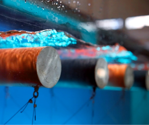
Waves were generated by a piston-type wavemaker (made by Delft Hydraulics Laboratory), driven by an electric motor. The input signal for regular waves was generated by in-house MATLAB-based scripts. The paddle is provided with three metallic plates, which limit the excitation of spurious transverse modes. The wave attenuation device consisted of an array of submerged floating cylinders (see figure 2), placed with their 58 cm axes parallel to the wave crests. The distance between the bottom of the flume and the top of the cylinder was set equal to 43 cm. Cylinders were made with commercial PVC pipes (with a diameter of 82 mm and wall thickness of 3 mm) filled with air. The tube ends were closed with 20 mm thick discs made of polyurethane foam and sealed with silicone caulk.

Figure 2. (a) Snapshot of an 11-cylinder device forced by regular waves of amplitude 2 cm and frequency 1.08 Hz, moving left to right. On the left side of the device, superposition of incident and reflected waves is visible. On the right, the wave attenuation can be observed. (b) Zoom-in on the first two cylinders.
Each inverted pendulum (sketched in figure 3) was anchored to the bottom with a wire of length  $l = 0.33$ m. The total density of each cylinder was
  $\rho _p = 220.27$ kg m
 $^{-3}$ (estimated from a total measured mass of 0.7 kg and a volume
  $V_p$ of 3168 cm
 $^3$), lower than that of the surrounding water
  $\rho _w = 997$ kg m
 $^{-3}$. The natural (resonance) frequency of the pendula
  $f_r$ was measured by tracking small oscillations, finding a mean common value of 0.6 Hz. More details on the method can be found in Appendix A.

Figure 3. Schematic of a single pendulum oscillating under the action of a regular wave, moving forward in the  $x$ direction. The vertical position of the pendulum shows the rest condition.
The cylinders were moored to two matching perforated steel angle bars ( $20\ {\rm mm} \times 20\ {\rm mm} \times 2\ {\rm mm}$), which were fixed to the concrete blocks on the flume bottom, (see figures 2 and 3), starting at 15.7 m from the wavemaker rest position. Each bar was 4 m long, with a series of holes 11.75 cm apart (indicated in the following as the
  $L^*$ parameter). The anchoring of each cylinder was made with four co-planar cables (made of galvanized steel with a diameter of 1.2 mm) connecting each tube end with both angle bars. This allowed the prevention of transverse horizontal motion.
The water surface elevation was measured with a commercial system (WG8USB, Edinburgh Designs Ltd.) capable of sampling the surface displacement with an accuracy of  $\pm$0.05 mm at a rate of 128 Hz via eight 700 mm long, resistance-type wave gauges. One wave gauge (WG1) was placed in the flume wave generation zone to monitor the wavemaker-generated waves. Another single gauge (WG8) was placed on the lee side of the device mounting zone to obtain measurements of the transmitted wave field. The remaining six gauges (WG2–WG7) were grouped into an array placed on the sea side of the device, with the last gauge located at 2.32 m from the first cylinder anchoring position. All the gauge positions (which are listed in table 1) were carefully chosen to be sufficiently far from any obstacle to prevent the capturing of localized evanescent modes. We used the gauge array (WG2–WG7) to obtain, via a least squares scheme (Zelt & Skjelbreia Reference Zelt and Skjelbreia1993), the linear incident and reflected surface elevation on the sea side of the device.
2.2. Experimental conditions
The device was composed of a number of cylindrical pendula placed at a regular distance, so as to maintain the periodic structure (see figure 2). The number of cylinders was tentatively designed to cover one wavelength corresponding to the natural frequency of the single pendulum  $f_r$, while maintaining a spacing
  $L$ sufficient to avoid possible direct collisions between two consecutive pendula. The 11-cylinder configuration can thus be thought as the smallest representative realization of a metamaterial, whose properties are usually studied for infinitely long arrays.
The test program (table 2) included various geometrical configurations in terms of number of cylinders  $N$, spacing between cylinders
  $L$, water depth
  $h$ and wave amplitude
  $a$. All spacings
  $L$ were multiples of the distance
  $L^*=11.75$ cm between adjacent holes in the perforated bars. With the aim of characterizing the frequency response of the device, each configuration was tested with approximately 30 regular long-crested wave conditions, with carrier frequency
  $f$ spanning between 0.4 and 1.4 Hz. Each single run was programmed to be 80 s long, including 3 s of initial ramp, starting at the still water condition, and the gauge acquisition duration was set to 160 s, starting 5 s before the onset of wave generation. The water depth considered in most of the runs was
  $h= 0.45$ m, while the top of the pendula was set to 0.43 m for all experiments. In these conditions, the submergence of the pendula (measured from the still water level and the top of the cylinder) is
  $d=2$ cm.
Table 2. Summary of the tests conducted in the lab. Each row represents a configuration which is defined by the number of pendula ( $N$), the water depth (
 $h$), the wave amplitude (
 $a$) and the spacing between two consecutive pendula (
 $L$). The latter is a multiple of
  $L^*=11.75$ cm. Each configuration has been tested under the same regular sea conditions for frequencies spanning the range from 0.4 to 1.4 Hz.

2.3. Wave analysis
The transmitted signal was measured with a single gauge (WG8) placed on the shore side of the device. Incident and reflected surface elevation were extracted by processing all signals measured by the six-gauge array, i.e. WG2–WG7 located on the offshore side of the device, by means of the least squares scheme proposed by Zelt & Skjelbreia (Reference Zelt and Skjelbreia1993), which considers that only free progressive modes exist in the flume. Incident, reflected and transmitted time series were then shortened to retain only the stationary state of the signals, i.e. the portion that is unaffected by wavemaker and beach reflections. For details on the specific application of the method and the strategy adopted, please see Appendix B.
Once the stationary portions of the incident, reflected and transmitted surface elevation were obtained, we estimated the reflection and the transmission coefficients  $C_R$ and
  $C_T$ as ratios between energies (spectral zeroth moments). From the energy balance, we derive the dissipation coefficient as
 \begin{equation} C_D = 1 - C_R - C_T. \end{equation}
3. Results
3.1. Dissipation
In figure 4, the dissipation coefficient, computed according to (2.1), is plotted against the frequency of the incident waves. In figure 4(a), each curve represents a configuration with the same spacing between the pendula,  $L=2L^*$, the same water depth, but a varying numbers of pendula. Regardless of the number of cylinders, large energy losses occurred in the band 0.6–0.8 Hz. When increasing the number of pendula (up to 11), the dissipation increases, especially in the band 0.6–0.8 Hz.

Figure 4. Dissipation coefficient as function of the wave frequency. (a) Each series represents a configuration with a different number of resonators, for  $L = 2L^*$,
  $a=0.01$ m and
  $d=2$ cm (i.e.
  $h = 0.45$ m). (b) Each series represents a different water level, for
  $L = 2L^*$,
  $a = 0.01$ m,
  $N = 11$ cylinders. The red-cross line is the same in both plots.
In figure 4(b), we consider the effect of the distance  $d$ between the still water level and the top of the cylinders on the dissipation. Each curve represents a different submergence while the device was fixed in a 11-cylinder configuration. Given the wave amplitude
  $a=1$ cm, for three out of four water levels, cylinders remained submerged both at rest and during the passage of the wave troughs. In these three cases, i.e.
  $h\geq 45$ cm (or equivalently
  $d \geq 2$ cm), large dissipation occurs in the same 0.6–0.8 Hz band. The behaviour is different in the case of lower water level (
 $h=43$ cm) corresponding to the slight emergence of the cylinders during the passage of the wave troughs. The maximum of energy dissipation occurs at lower frequencies, below the modal one. In the high frequency tail,
  $f>0.9$ Hz, it appears that the more submerged the cylinders are, the lower the resulting dissipative capacity is.
In figure 5, the role of the cylinder spacing  $L$ is considered. Panels (a), (b) and (c) depict the results for configurations with
  $L=2 L^*$,
  $4 L^*$ and
  $7 L^*$, respectively. Each line represents
  $C_D$ referring to different number of pendula
  $N$. In general, for any
  $L$, energy losses increase with the number of cylinders. Moreover, the shape of the main dissipation bump in the 0.6–0.8 Hz band is similar for any
  $L$, experiencing a slight shift towards lower frequencies as
  $L$ increases. However, in the high-frequency region,
  $f>0.9$ Hz, a different value of
  $L$ corresponds to a different response curve, and the shape of the response is unaffected by the number of cylinders. Specifically, taking
  $L=2 L^*$ as the baseline, an increase of the pendula spacing corresponds to the appearance of dissipation peaks at specific frequencies. Regardless of the number of pendula, for
  $L=4 L^*$, these peaks locate at around 1.0 Hz and 1.15 Hz. The similarities between the three- and four-cylinder line are also clear for
  $L=7 L^*$.

Figure 5. Dissipation coefficient for various geometrical configurations and varying the number of pendula: (a)  $L=2L^*$; (b)
  $L=4L^*$ and (c)
  $L=7L^*$.
Wave amplitudes also play a role: in figure 6(a), the response of the 11-cylinder configuration is taken as the reference, for  $L=2L^*$, a 0.45 m water depth, excited by small amplitude waves
  $a=1$ cm, as already depicted in figure 5. The other two lines refer to wave amplitudes
  $a = 2$ cm and
  $a = 3$ cm, respectively. In general, larger amplitude waves correspond to a flatter response curve. Within the 0.6–0.8 Hz band, the dissipation decreases with the wave amplitude. In contrast, higher energy dissipation takes place for shorter and longer waves. Note that, especially for
  $a=3$ cm, but also in some cases with
  $a=2$ cm, at least the first two or three cylinders emerged above the water during the passage of the wave troughs.

Figure 6. Dissipation coefficient for 11 cylinders,  $L = 2L^*$,
  $h=0.45$ m and three different incoming wave amplitudes: (a) as function of the wave frequency and (b) as function of the wave steepness.
Figure 6(b) depicts the same data of figure 6(a) plotted against the wave steepness  $ka$. The only clear behaviour that can be observed is the general increase of dissipation with increasing
  $ka$. Indeed, as will be discussed later on, the most relevant effects are influenced by the local steepness at the interaction, and only indirectly by that of the incoming wave.
3.2. Off-shore reflection
While energy dissipation appears smooth across the tested frequency range, the amount of energy reflected back off-shore is concentrated at relatively sharp peaks.
Figure 7 shows  $C_R$ for different configurations, namely
  $L=2L^*$ in panel (a),
  $L=4L^*$ in panel (b) and
  $L=7L^*$ in panel (c). As in figure 5, each panel depicts the response of three, four and five cylinders. In general, the device is scarcely capable of reflecting back the incoming energy, except at specific frequencies, where sharp peaks appear. These peak positions do not vary with the number of cylinders. Only the height of the peaks, i.e. the amount of reflected energy, appears slightly larger if the number of cylinders in the array is greater. This is what we observe in general, except for a particular situation in figure 7. Here, the
  $C_R$ peak of the
  $N=4$ case (around
  $f=1.1$ Hz) is higher than the
  $N=5$ cases, but the difference is smaller than the experimental error.

Figure 7. Reflection coefficients for the same configurations as in figure 5.
Each geometrical configuration displays its own peculiar frequency response. Increasing the cylinder spacing, the high reflection ( $C_R>0.4$) peaks migrate to lower frequencies.
To investigate the effects of pendula submergence, figure 8 documents a configuration (11 cylinders,  $L=3L^*$) not considered in previous plots. This is useful for the interpretation of the reflection patterns, and is discussed in § 4.1. Reflection was almost negligible if the pendula rest position corresponded to the still water level,
  $d=0$. If the device was sufficiently submerged, the reflection coefficient presented localized peaks, similar to those observed in figure 7. Except in a small interval around
  $f=1.2$ Hz, where the behaviour is not sufficiently clear, both locations and intensities of the mid-frequency peak (around 0.85 Hz) and the high-frequency peak (
 $f\geq 1.4$ Hz) are likely to be independent on the level of immersion.

Figure 8. Reflection coefficients for 11 cylinders,  $h=0.45$ m,
  $a=1$ cm for two different spacing: (a)
  $L=2L^*$; (b)
  $L=3L^*$.
3.3. Nearshore transmission
On the nearshore side of the device, transmitted waves were measured using a single gauge. While dissipation and reflection measurements are important to understand the fluid dynamics around the pendula, transmission returns the residual energy of the incoming wave after the interaction with the device, providing an overall indication of the effectiveness of the system. Smaller transmission coefficients correspond to better energy wave attenuation.
In figure 9, the transmission coefficients  $C_T$ are plotted as function of the incident wave frequency for the same configurations depicted in figure 5 (dissipation) and figure 7 (reflection). Similarly, for the most investigated configuration
  $L=2L^*$, we present in figure 10 the transmission results for varying number of cylinders, which can be compared with figure 4(a) (dissipation) and figure 8 (reflection).

Figure 9. Transmission coefficients for various geometrical configurations and varying number of pendula: (a)  $L=2L^*$; (b)
  $L=4L^*$ and (c)
  $L=7L^*$.

Figure 10. Transmission coefficients with  $d=2$ cm,
  $a=1$ cm,
  $L=2L^*$ for different array configurations by varying the number of the pendula.
4. Discussion
4.1. Generalized Bragg scattering analysis: the effect of the spacing between cylinders
Liu & Yue (Reference Liu and Yue1998) analysed the interaction of surface gravity waves over a wavy bottom, providing the conditions for generalized Bragg scattering. This mechanism is very similar to the one that describes the nonlinear interactions of surface gravity waves pioneered by Phillips (Reference Phillips1960) and by Hasselmann (Reference Hasselmann1962). Energy can be transferred from one mode to another when the so-called resonant condition occurs at some order. To have an efficient transfer of energy among  $M$ modes, the following condition must be met:
 \begin{equation} \left.\begin{array}{c} k_1\pm k_2\pm \cdots \pm k_M=0\\ \omega_1 \pm \omega_2 \pm \cdots \pm \omega_M=0 \end{array}\right\}, \end{equation}
with
 \begin{equation} \omega_i=\omega(k_i)=2{\rm \pi} f_i=\sqrt{g |k_i| \tanh (|k_i| h)}. \end{equation}
The theory is quite involved and details are provided by Nazarenko (Reference Nazarenko2011). The number of waves that are interacting depends on the degree of nonlinearity of the system, which is  $M-1$. For example, for pure gravity waves, the first resonant interaction is for
  $M=4$, i.e. the dynamical equations are characterized by a cubic nonlinearity. In the presence of a structure, in addition to mutual interaction, waves interact with it. If the structure is periodic, then one can generalize the described resonant process, and take one of the wavenumbers in (4.1) as the one associated with the spatial periodicity of the structure, which is considered fixed (clearly, its associated frequency is zero).
In our case, the pendula are separated by a distance  $L$; therefore, we can consider a periodic structure characterized by a wavenumber
  $k_{L}=2{\rm \pi} /L$. Moreover, we neglect the motion of the pendula. Thus, by combining wavenumbers of surface gravity waves with the wavenumber of the periodic structure, we obtain general conditions for Bragg scattering at the desired order. The simplest is the standard Bragg scattering for which we take
  $M=3$: two wavenumbers associated with surface waves and one from the fixed structure to obtain
 \begin{equation} \left.\begin{array}{c} k_1\pm k_2\pm k_L=0\\ \omega_1\pm \omega_2=0 \end{array}\right\}. \end{equation}
From these equations, we get that the only solution, since  $\omega \ge 0$, is
  $k_1=-k_2=k$, which implies
  $2k=k_L$, i.e. the classical Bragg scattering. Higher order interactions are possible.
In the same way, for  $M \geq 3$, admitting only the existence of two waves having the same frequency and travelling in opposite directions, we have the generalized Bragg resonance condition
 \begin{equation} 2 k = n k_L, \end{equation}
with  $n \in \mathbb {N}$. For any
  $n \ge 1$, this condition states that there is a possible energy transfer from the incoming wave,
  $k$, to the backward travelling one,
  $-k$, i.e. the device reflects the energy.
In a wave flume experiment, even dealing with small amplitude regular waves, we cannot neglect the existence of higher harmonics. The wavemaker sinusoidal motion used in this study causes the release of spurious components, the bigger ones being second harmonics that have the same order of magnitude of the Stokes bound modes, but travel at their own speed, i.e. their wavenumber is determined by (4.2) (see e.g. Schaffer Reference Schaffer1996). Also, Grue (Reference Grue1992) and Chaplin (Reference Chaplin1984), in the case of a single submerged cylinder, observed the generation of the second and third harmonics. Therefore, we can expect that similar effects take place also for waves interacting with the pendula array, and admit that if  $\omega$ is the frequency of the fundamental wave, higher harmonics may be travelling in the flume, satisfying the dispersion relation
 \begin{equation} m \omega = \sqrt{g k^{(m)} \tanh{h k^{(m)}}},\quad m\in\mathbb{N}, \end{equation}
where the apex in parenthesis indicates the order of the harmonic. Including these waves into the resonance conditions, we find interactions of the type:
 \begin{equation} 2 k + k^{(2)} = n k_L, \end{equation}
and a number of other conditions. These include for example the Bragg resonances of the second harmonic, and other situations, which require that the wavemaker-generated second harmonic be large enough. This is not our case, at least in small amplitude tests. However, the condition (4.6) takes into account second harmonics travelling back to the wavemaker, after being ‘generated’ from the interaction of the carrier with the pendula lattice. Table 3 summarizes the first solutions of the generalized Bragg condition (4.4) and second harmonic reflection (4.6). Around these frequencies, the most significant peaks in the reflection coefficients, presented in § 3.2, can be observed. To facilitate the interpretation, we reproduce some of the above results in figure 11. Here, the reflection coefficients are given for the fundamental frequency  $f$ and the second harmonic (
 $2f$), both with reference to the incoming energy of the fundamental. The four panels reproduce the four geometrical configurations, with different
  $L$ values. The number of cylinders is also different, but it is not significant for the present analysis. Around the blue lines (Bragg scattering conditions), the reflection is relevant and almost all the energy is transferred to the reflected fundamental, testifying a Bragg-like scattering effect. Around the red lines, the reflected second harmonic is strongly enhanced, while the fundamental is very small. This confirms the predictions of (4.6). As pointed out in the review by Patil & Matlack (Reference Patil and Matlack2021), this second harmonic generation effect is a typical nonlinear phenomenon linked to the geometrical configuration of the device (see also Guo et al. Reference Guo, Gusev, Tournat, Deng and Bertoldi2019; Raju et al. Reference Raju, Lee, Liu, Zhu, Zhu, Poutrina, Urbas and Cai2022). Indeed, in our tests this behaviour can be observed even for very small amplitude incident waves (i.e. linear regime). Notice that the magnitude of the reflection peaks appears to decay with larger
  $L$, as the generalized Bragg resonant frequencies become smaller. Moreover, for longer waves, close to the cylinder natural frequency, waves directly excite the motion of the pendula that, moving in a viscous fluid, generate a turbulent wake whose kinetic energy is then dissipated into heat in the bulk of the medium.
Table 3. Scattering frequencies for (fixed) cylinder array with spacing  $L$ (rows). First two exact solutions of (4.4) (Bragg scattering) and (4.6) (second harmonic generation).


Figure 11. Reflection coefficients for the fundamental (dots, solid) and second harmonic (crosses, broken line): (a)  $L=2L^*$,
  $N = 11$; (b)
  $L=3L^*$,
  $N=11$; (c)
  $N=5$,
  $L=4L^*$; (d)
  $N=5$,
  $L=7L^*$. Blue, Bragg scattering frequencies (4.4); red, second harmonic generation (4.6). Note that ordinate axis scales with a quadratic power law.
4.2. Effect of the number of cylinders
The dissipation coefficient is large, for all configurations, in the same 0.6–0.8 Hz band. For the submerged device ( $d>0$ in figure 4b), the behaviour of the resonance frequency band does not change with the water level, and its position depends mainly on the characteristics of the single pendula.
According to (2.1), the dissipation must be interpreted as total energy loss, which not only depends on the energy exchanges in water but also between water and air, and the damping of the flume bottom and walls.
Overall, it appears that the frequency at which dissipation takes place depends on the single cylinder behaviour. Indeed, the total energy loss increases with the number of elements (see figures 4(a) and 5), while, fixing all other variables, the response curves are similar. In summary, increasing the number of cylinders leads to a decrease of the transmitted energy to the shore in the whole frequency range (see § 3.3). If the number of cylinders is sufficiently large, all the incoming energy, in a frequency interval around the resonant frequency, can be dissipated. The dissipation is probably the result of the presence of a band gap associated with the local resonance mechanism that excites the motion of the cylinders which dissipate energy into water (see figure 10 in the region 0.6–0.8 Hz).
4.3. Submergence of the cylinders and dependence on wave amplitude
During the experiments, it has been visually observed that for wave amplitudes larger than the baseline (1 cm), at least the first or the second cylinders were always exposed to air during the tests (see videos in the supplementary movies available at https://doi.org/10.1017/jfm.2023.741). There are two clear effects that depend on the submergence of the pendula. The first relates to its dissipative capacity, as can be observed in figure 4(b). For all fully submerged configurations, most of the dissipation occurs at frequencies which are just above the natural frequency of the pendula, but for  $d=0$ (the cylinders are fully immersed only with the water at rest), the dissipation peak moves towards longer waves. This is consistent with previous studies (Sergiienko et al. Reference Sergiienko, Cazzolato, Ding, Hardy and Arjomandi2017) showing how, for long waves, an emerging device is more effective. Also, shorter waves lose significant energy only if the wave amplitude (1 cm in this case) is comparable with the distance between the mean water level and the top of the cylinders. Thus, in the high-frequency range (above 1 Hz), less immersed devices are more effective. This is probably due to surface breaking effects, clearly observed during these tests, which can become important for small submergence. The second effect is visible in both panels of figure 8. As discussed, the peaks around 1.1 Hz and 0.95 Hz (panels (a) and (b), respectively) are due to second harmonic generation. If the cylinders are not fully immersed (
 $d=0$ lines), no reflection peak is observed, meaning that the second harmonic generation mechanism is triggered only if the pendula are fully immersed.
Increasing the wave amplitude, while keeping the same mean water level, the frequency response does not change drastically. The curves flatten, with short waves losing more energy, but the high dissipation in the 0.6–0.8 Hz range remains. Increasing wave amplitude leads to the onset of other mechanisms, such as wave breaking and other nonlinear phenomena, thus making the behaviour of the device more complex (see the supplementary movies).
For a given frequency, as the amplitude increases, the steepness becomes larger and the waves have more probability of breaking, especially at the edge of the device where the local amplitude becomes larger. Thus, in general, a higher steepness of the incoming wave will result in a higher dissipation coefficient (figure 6b). However, despite the steepness of the generated wave being clearly a proxy for nonlinear phenomena occurring in waves, it is not a clear indicator of the dissipative phenomena occurring in our complex system, for which, most likely, the local steepness, due to amplification effects, play a major role.
The above analysis captures almost all the features in the transmission and reflection spectra, but it does not explain the observed behaviour in the interval 1.2–1.3 Hz. In this range, there is small but finite reflection in all configurations. We note that the frequency of 1.2 Hz corresponds to twice the natural frequency of the pendulum, but is also close to the channel first transverse mode (see e.g. Tulin & Waseda Reference Tulin and Waseda1999). During the tests with frequencies close to 1.2 Hz, we actually observed the excitation of non-negligible transverse modes, causing the first one or two pendula to rotate on the horizontal plane.
5. Conclusions
This work draws its motivation from the attempt to address the problem of coastal erosion. The idea is to exploit the concept of metamaterial wave control, building a device to mitigate surface gravity waves. In particular, the objective is to exploit both local resonance effects and Bragg scattering from a periodic array of structures to obtain band gaps, hence, attenuation in a wide frequency range. Following numerical results presented by De Vita et al. (Reference De Vita, De Lillo, Bosia and Onorato2021a), we experimentally investigated a first prototype in a wave flume using an array of submerged and inverted cylindrical pendula. We performed single-frequency wave tests over a wide range of frequencies, aiming to maintain the system in the linear regime as far as possible. Experiments were carried out varying various parameters, including the spacing  $L$, the number of pendula, their submergence and the amplitude of the incoming waves.
Results demonstrated the feasibility of the concept, and that wave attenuation can be significant even using a limited number of cylinders and without any particular optimization. In the experiments, wave energy attenuation reached 80 % over a large range of frequencies in the case of 11 cylinders. In this configuration, the submerged device ceased to be effective only in attenuating very long waves. Analysis of results allowed us to assess how the two leading mechanisms (local resonance and generalized Bragg scattering) contribute to wave attenuation. The main discriminant is the submergence of the device. If the pendula are fully immersed, a gap around the resonance frequency is observed, while non-fully immersed pendula attenuate both longer and shorter waves. It remains to be understood in this case if the natural frequency of the pendula played a role. Most likely, the proper frequency of oscillation of a pendulum changes when it is semi-immersed. The scattering behaviour is also different if the pendula are immersed or not. Only in the former case, some of the incoming energy is prevented from propagating through the array, and is reflected back to sea. This occurs in narrow bands close to four and five wave interaction frequency conditions (including harmonics), which depend on the geometry of the whole structure, with Bragg scattering being only the simplest mechanism.
We stress that the dynamics involved in the problem is rather complex: the response of the system is the result of an interplay of scattering by a regular array (Bragg scattering), local resonance of the pendula, nonlinear transfer of energy and turbulent dissipation. More specifically, water is a viscous fluid and dissipation is dominant at some frequencies; nonlinearity, turbulence, and effects like wave breaking are not negligible in our study. The representation of all these phenomena in numerical experiments, for example by means of computational fluid dynamics or smoothed particle hydrodynamics, is still a challenging task, especially if one wishes to simulate the extensive set of tests presented in this paper. Certainly, some of the features observed in this experimental work can be reproduced with linearized potential flow equations. However, a theoretical analysis describing the interplay between the phenomena mentioned is by far not a simple task, and it will be the subject of future studies.
Regarding the feasibility of appropriately designing the cylinder array, an optimal device should prevent or mitigate the propagation of waves to the shore for a particular wave climate. Appropriate choice of geometrical parameters can allow to tune band gap frequencies to desired values. The local resonance gap can be adjusted by appropriate choice of pendulum parameters, since it is mainly related to their natural oscillation frequency. It is expected that, at prototype scale, dissipation will vary compared with that observed in the lab. Thus, to move to a proof of concept device, it is necessary to properly understand the scaling of viscous effects and verify if they remain relevant for real sea conditions. We have also seen that when pendula remain completely submerged, wave scattering is relevant around frequencies that can be predicted by Bragg scattering relations. It should be possible to tune the position of the reflection bands by modifying the spacing of the pendula.
Overall, the presented design concept appears promising in the quest to realize a new class of multi-frequency surface gravity wave absorbers with increased efficiency and limited environmental impact, to be applied, e.g. for the protection against beach erosion in practical scenarios.
Supplementary movies
Supplementary movies are available at https://doi.org/10.1017/jfm.2023.741.
Acknowledgements
The authors wish to thank C. Manes and C. Camporeale for their valuable suggestions during the early stages of the work and for providing access to the laboratory, G.F. Caminiti for his help in setting up the experimental apparatus, and Vito Jr. Battista for producing photographs and video material.
Funding
This work has been funded by Compagnia di San Paolo Progetto d'Ateneo – Fondazione San Paolo Metapp, no. CSTO160004, and Proof of concept Metareef grant. M.O., F.B., F.D.L. and M.L. acknowledge the EU, H2020 FET Open Bio-Inspired Hierarchical MetaMaterials (grant number 863179) and the Departments of Excellence grant (MIUR). M.O. acknowledges funding from the Italian Ministry of University and Research (PRIN 2020 2020X4T57A). M.O. was supported by Simons Collaboration on Wave Turbulence, grant no. 617006.
Declaration of interests
The authors report no conflict of interest.
Appendix A
To measure the proper frequency of oscillation of the pendula in water and its dissipation features, we installed a single cylinder in the flume. In calm water conditions, it was displaced slightly from its equilibrium position, by an amount compatible with the small angle approximation, and then released to initiate free oscillations. In the meantime, the motion of the pendulum was recorded using a high-resolution camera, sampling at 50 frames per second. The video recording was processed by means of a Python 3 script integrating the Open-CV library (Bradski Reference Bradski2000). First, the images were calibrated using a chessboard placed on the glass of the wave flume, and then the centre position of the lateral section of the pendulum was identified frame by frame. By doing so, we obtained a time series for the angle  $\vartheta$, i.e. the angle between the pendulum wire and the vertical axis (see figure 3).
Assuming linear damping and small oscillations, we can describe the motion of the free pendulum in terms of  $\vartheta$, i.e. the angle between the pendulum wire and the vertical axis, as
 \begin{equation} \frac{{\rm d}^2\vartheta}{{\rm d} t^2} + 2\beta \frac{{\rm d}\vartheta}{{\rm d}t} + {\omega_r}^2 \vartheta =0, \end{equation}
where  $\beta$ is the damping coefficient and
  $\omega _r=2{\rm \pi} f_r$ is the natural frequency of the undamped pendulum. The general solution of (A1) consists of a sinusoidal oscillation with gradually decreasing amplitude (see e.g. Symon Reference Symon1971), that is,
 \begin{equation} \vartheta = \vartheta_0 \, {\rm e}^{-\beta t} \cos{(\omega_1 t + \phi)}, \end{equation}
with  $\vartheta _0$ and
  $\phi$ two arbitrary constants fixed by the initial conditions, and the damped circular frequency defined as
 \begin{equation} \omega_1^2 = \omega_r^2-\beta^2. \end{equation}
Equation (A2) was fitted to the experimental data by means of the Levenberg–Marquardt least squares method (Dennis & Schnabel Reference Dennis and Schnabel1996). An example is shown in figure 12, while the results, averaged among five distinct tests, are reported in table 4.

Figure 12. Example of a damped oscillation test. The blue broken line represents the data series acquired with the tracking method, while the red solid line represents the fitted curve using (A2).
Table 4. Results of the fitting method, with  $f_r$ obtained substituting the fitted parameter
  $\omega _1$ in (A3).
The frequency can also be estimated analytically; the procedure to be explained below can be used for designing resonators in conditions characterized by different water depth or length of the pendula. When a body of mass  $M$ in a fluid is subjected to an acceleration
  $a_b$, the fluid around the body is also accelerated. Thus, the total kinetic energy is given by two terms and the total force
  $F$ will be
 \begin{equation} F = (M+m) a_b, \end{equation}
where  $m$ is the so-called added mass. The latter depends on the volume
  $V$ of fluid displaced, on its density
  $\rho _w$, and on coefficient
  $c$ that depends on the shape of the body, the water depth and the incident wave frequency,
  $m=c \rho _w V$. It is straightforward to show that the angular frequency of oscillation of a free pendulum in a fluid is given by
 \begin{equation} \omega_r = \omega_a \sqrt{\frac{\rho_w - \rho_p}{ \rho_p + c \rho_w}}, \end{equation}
where  $\rho _p$ is the cylinder density,
  $\omega _a = \sqrt {g/(l+R)}$, with
  $l$ the wire length,
  $R$ the radius of the cylinder and
  $g$ the gravitational acceleration. Using our experimental value of the resonant frequency, we can estimate the added mass coefficient to be
  $c \approx 1.25$.
Appendix B
We outline here the strategy adopted in the measurement post-processing, since this information is crucial for the repeatability of the experiments.
First of all, there are a number of features that are common to all test signals, as can be seen in the example shown in figure 13. After the initial rest phase, there is a wavemaker ramp-up of a few oscillations, followed by a further two or three wave periods for the system to reach a stationary state (highlighted in figure 13), which is the portion of signal of interest. After a stationary phase, the state is perturbed by reflected waves from either the wavemaker or the flume end.

Figure 13. Example of surface elevation time series acquired on the sea side of the pendula array (broken light grey line). The solid dark line highlights the stationary time series used to assess the main properties.
The signals measured at the six-gauge array (WG2–WG7) were processed to obtain separated incident and reflected progressive waves. The separation algorithm is based on the least squares scheme proposed by Zelt & Skjelbreia (Reference Zelt and Skjelbreia1993), which considers that only free progressive modes exist in the flume.
As can be deduced from table 2, according to weakly nonlinear theory (see e.g. Whitham Reference Whitham1974) the amplitude of the second order bound modes in the channel were at most 1 % of the amplitude of the carrier wave, so the overall error in estimating them as free modes is negligible.
Moreover, in order to avoid contamination of the measurements by evanescent modes, all gauges were placed sufficiently far from the obstacles.
A purely linear approach was thus sufficient to analyse the stationary parts of the signals, but, given the presence of transients (figure 13), the application of the least squares scheme to the whole time series would introduce non-physical artefacts. To avoid this, localized and overlapped portions of the signals were processed using a sliding Hann window (Engelberg Reference Engelberg2008). The window length was designed to be approximately equal an integer number of periods, also oversampling the signal according to a first estimation of the main wave period. Moreover, the start and end of the series were artificially extended with additional zeros, to sufficiently resolve the frequency domain and thus correctly estimate the wavenumbers.
As mentioned above, in all experiments, only the stationary signal was considered for data processing, excluding all transient states. Thus, in each test, a different number of waves was analysed, depending on the associated wavelength, the truncated signal length being the same for incident, reflected and transmitted time series. In any case, the maximum possible number of wave periods was considered, allowing a more robust estimation of the desired quantities at higher frequencies.
Figure 14 shows an example of a time series for a wave with an amplitude of 2 cm and frequency of 0.97 Hz interacting with 11 cylinders moored with  $2L^*$ mutual spacing. The grey-scale time series (figure 14a) represents the signal acquired by WG1, the red line (figure 14b) shows the incident waves, the waves reflected by the device are depicted by in green (figure 14c) and figure 14(d) is dedicated to the transmitted waves at the shore-side of the device (blue). Note that the incident wave time series is also replicated for visual comparison in figures 14(c) and 14(d).

Figure 14. Example of (a) generated, (b) incident, (c) reflected and (d) transmitted waves. In panels (c) and (d), the additional dotted-red line represents the reconstructed incident wave field. Panels have different abscissas corresponding to different transit times of the same wave crest at the gauges of reference, i.e. WG1 for panel (a), WG2 for panels (b) and (c), and WG8 for panel (d). Clearly, the incident wave at WG8 is an artefact included for visual comparison.


 Open access