2.1. Hydrodynamical model

We consider a non-rotating spherical shell of inner radius $r_i$ and outer radius $r_o$ with $r_i/r_o=0.35$ filled with a Newtonian Boussinesq fluid of background density $\rho _c$. The spherical-shell boundaries are assumed to be impermeable, no slip and held at constant temperature and chemical composition. The kinematic viscosity $\nu$, the thermal diffusivity $\kappa _T$ and the diffusivity of chemical composition $\kappa _\xi$ are assumed to be constant. We adopt the following linear equation of state:

(2.1)\begin{equation} \rho = \rho_c [1-\alpha_{T}(T - T_c) -\alpha_{\xi}(\xi - \xi_c)], \end{equation}

which ascribes changes in density ($\rho$) to fluctuations of temperature ($T$) and chemical composition ($\xi$). In the above expression, $T_c$ and $\xi _c$ denote the reference temperature and composition, while $\alpha _T$ and $\alpha _\xi$ are the corresponding constant expansion coefficients. In the following, we adopt a dimensionless formulation using the spherical-shell gap $d=r_o-r_i$ as the reference length scale and the viscous diffusion time $d^2/\nu$ as the reference time scale. Temperature and composition are respectively expressed in units of $\Delta T=T_{{top}}-T_{{bot}}$ and $\Delta \xi =\xi _{{bot}}-\xi _{{top}}$, their imposed contrasts over the shell. The dimensionless equations which govern the time evolution of the velocity $\boldsymbol {u}$, the pressure $p$, the temperature $T$ and the composition $\xi$ are expressed by

(2.2)$$\begin{gather} \boldsymbol{\nabla} \boldsymbol{\cdot} \boldsymbol{u} = 0, \end{gather}$$

(2.3)$$\begin{gather}\dfrac{\partial \boldsymbol{u}}{\partial t} + \boldsymbol{u} \boldsymbol{\cdot}\boldsymbol{\nabla}\boldsymbol{u} =- \boldsymbol{\nabla} p +\dfrac{1}{Pr}\left(-Ra_T T + \dfrac{Ra_\xi}{Le} \xi \right) g \boldsymbol{e}_r + \nabla^2 \boldsymbol{u}, \end{gather}$$

(2.4)$$\begin{gather}\dfrac{\partial T}{\partial t} + \boldsymbol{u} \boldsymbol{\cdot} \boldsymbol{\nabla} T = \dfrac{1}{Pr}\nabla^2 T, \end{gather}$$

(2.5)$$\begin{gather}\dfrac{\partial \xi}{\partial t} + \boldsymbol{u} \boldsymbol{\cdot} \boldsymbol{\nabla} \xi = \dfrac{1}{Le Pr} \nabla^2 \xi, \end{gather}$$

where $\boldsymbol {e}_r$ is the unit vector in the radial direction and $g=r/r_o$ is the dimensionless gravity. The set of equations (2.2)–(2.5) is governed by four dimensionless numbers

(2.6a–d) \begin{equation} Ra_T =-\dfrac{\alpha_T g_o d^3 \Delta T}{\nu \kappa_T}, \quad Ra_\xi = \dfrac{\alpha_\xi g_o d^3 \Delta \xi}{\nu \kappa_\xi}, \quad Pr = \dfrac{\nu}{\kappa_T}, \quad Le = \dfrac{\kappa_T}{\kappa_\xi}, \end{equation}

termed the thermal Rayleigh, chemical Rayleigh, Prandtl and Lewis numbers, respectively. Our definition of $Ra_T$ makes it negative, in order to stress the stabilising effect of the thermal background. For the sake of clarity, we will also make use of the Schmidt number $Sc=\nu /\kappa _\xi =Le\,Pr$ in the following. The stability of the convective system depends on the value of the density ratio $R_\rho$ (Stern Reference Stern1960) defined by

(2.7)\begin{equation} R_\rho = \dfrac{\alpha_T \Delta T}{\alpha_\xi \Delta \xi}, \end{equation}

which relates to the above control parameters via $R_\rho = Le |Ra_T|/Ra_\xi$. In order to compare models with different Lewis numbers $Le$, it is convenient to also introduce a normalised density ratio $r_\rho$ following Traxler, Garaud & Stellmach (Reference Traxler, Garaud and Stellmach2011a)

(2.8)\begin{equation} r_\rho = \dfrac{R_\rho - 1}{Le - 1}. \end{equation}

This maps the instability domain for fingering convection, $1\leq R_\rho < Le$, to $0\leq r_\rho <1$.

2.2. Numerical technique

We consider numerical simulations computed using the pseudo-spectral open-source code MagIC (freely available at https://github.com/magic-sph/magic) (Wicht Reference Wicht2002). MagIC has been validated against a benchmark for rotating double-diffusive convection in spherical shells initiated by Breuer et al. (Reference Breuer, Manglik, Wicht, Trümper, Harder and Hansen2010). The system of equations (2.2)–(2.5) is solved in spherical coordinates $(r,\theta,\phi )$, expressing the solenoidal velocity field in terms of poloidal ($W$) and toroidal ($Z$) potentials

(2.9)\begin{equation} \boldsymbol{u} = \boldsymbol{u}_P+\boldsymbol{u}_T = \boldsymbol{\nabla} \times( \boldsymbol{\nabla} \times W\,\boldsymbol{e}_r) + \boldsymbol{\nabla} \times Z\,\boldsymbol{e}_r. \end{equation}

The unknowns $W$, $Z$, $p$, $T$ and $\xi$ are then expanded in spherical harmonics up to the maximum degree $\ell _{max}$ and order $m_{max}=\ell _{max}$ in the angular directions. Discretisation in the radial direction involves a Chebyshev collocation technique with $N_r$ collocation grid points (Boyd Reference Boyd2001). The equations are advanced in time using the third-order implicit–explicit Runge–Kutta schemes ARS343 (Ascher, Ruuth & Spiteri Reference Ascher, Ruuth and Spiteri1997) and BPR353 (Boscarino, Pareschi & Russo Reference Boscarino, Pareschi and Russo2013) which handle the linear terms of (2.2)–(2.5) implicitly. At each iteration, the nonlinear terms are calculated on the physical grid space and transformed back to spectral representation using the open-source SHTns library (freely available at https://gricad-gitlab.univ-grenoble-alpes.fr/schaeffn/shtns) (Schaeffer Reference Schaeffer2013). The seminal work by Glatzmaier (Reference Glatzmaier1984) and the more recent review by Christensen & Wicht (Reference Christensen and Wicht2015) provide additional insights into the algorithm (the interested reader may also consult Lago et al. (Reference Lago, Gastine, Dannert, Rampp and Wicht2021) with regard to its parallel implementation).

2.3. Diagnostics

We introduce here several diagnostics that will be used to characterise the convective flow and the thermal and chemical transports. We hence adopt the following notations to denote temporal and spatial averaging of a field $f$:

(2.10a–c)\begin{align} \bar{f} = \dfrac{1}{t_{avg}}\int_{t_0}^{t_0+t_{{avg}}} f \,\mathrm{d}t,\quad \langle\, f \rangle_V = \dfrac{1}{V}\int_V f\,\mathrm{d}V, \quad \langle\, f \rangle_S = \dfrac{1}{4{\rm \pi}}\int_0^{2{\rm \pi}}\int_0^{\rm \pi} f\,\sin\theta \,\mathrm{d}\theta\,\mathrm{d}\phi, \end{align}

where time averaging runs over the interval $[t_0,t_0+t_{{avg}}]$, $V$ is the spherical shell volume and $S$ is the unit sphere. Time-averaged poloidal and toroidal energies are defined by

(2.11a,b)\begin{equation} E_{{k}, {pol}} = \dfrac{1}{2}\overline{\langle \boldsymbol{u}_P\boldsymbol{\cdot}\boldsymbol{u}_P \rangle_V} = \sum_{\ell=1}^{\ell_{max}} E_{{k}, {pol}}^{\ell}, \quad E_{{k}, {tor}} = \dfrac{1}{2}\overline{\langle\boldsymbol{u}_T\boldsymbol{\cdot}\boldsymbol{u}_T \rangle_V} = \sum_{\ell=1}^{\ell_{max}} E_{{k}, {tor}}^{\ell} , \end{equation}

noting that both can be expressed as the sum of contributions from each spherical harmonic degree $\ell$, $E_{{k}, {pol}}^{\ell }$ and $E_{{k}, {tor}}^{\ell }$. The corresponding Reynolds numbers are then expressed by

(2.12a,b)\begin{equation} Re_{pol} = \sqrt{2E_{{k}, {pol}}}, \quad Re_{tor}=\sqrt{2E_{{k}, {tor}}}. \end{equation}

In the following we also employ the chemical Péclet number, $Pe$, to quantify the vertical velocity. It relates to the Reynolds number of the poloidal flow via

(2.13)\begin{equation} Pe = Re_{pol}\,Sc. \end{equation}

We introduce the notation $\varTheta$ and $\varXi$ to define the time and horizontally averaged radial profiles of temperature and chemical composition

(2.14a,b)\begin{equation} \varTheta = \overline{\langle T \rangle_S},\quad \varXi = \overline{\langle \xi \rangle_S}. \end{equation}

Heat and chemical composition transports are defined at all radii by the Nusselt $Nu$ and Sherwood $Sh$ numbers

(2.15a,b)\begin{equation} Nu = \dfrac{\overline{\langle u_r T \rangle_S}- \dfrac{1}{Pr}\dfrac{\mathrm{d} \varTheta}{\mathrm{d} r}}{-\dfrac{1}{Pr}\dfrac{\mathrm{d} T_c}{\mathrm{d} r}}, \quad Sh = \dfrac{\overline{\langle u_r \xi \rangle_S}-\dfrac{1}{Sc} \dfrac{\mathrm{d} \varXi}{\mathrm{d} r}}{-\dfrac{1}{Sc}\dfrac{\mathrm{d} \xi_c}{\mathrm{d} r}}, \end{equation}

where $\mathrm {d}T_c /\mathrm {d} r = r_i r_o/r^2$ and $\mathrm {d}\xi _c /\mathrm {d} r = -r_i r_o/r^2$ are the gradients of the diffusive states. In the numerical computations, those quantities are practically evaluated at the outer boundary, $r=r_o$, where the convective fluxes vanish. Heat sinks and sources in fingering convection are provided by buoyancy power of thermal and chemical origins $\mathcal {P}_T$ and $\mathcal {P}_\xi$, expressed by

(2.16a,b)\begin{equation} \mathcal{P}_T = \dfrac{|Ra_T|}{Pr}\overline{\langle g u_r T \rangle_V},\quad \mathcal{P}_\xi = \dfrac{Ra_\xi}{Sc}\overline{\langle g u_r \xi \rangle_V}. \end{equation}

On time average, the sum of these two buoyancy sources balances the viscous dissipation $D_\nu$ according to

(2.17)\begin{equation} \mathcal{P}_T + \mathcal{P}_\xi = D_\nu, \end{equation}

where $D_\nu =\overline {\langle (\boldsymbol {\nabla }\times \boldsymbol {u})^2 \rangle _V}$.

As shown in Appendix B, the thermal and compositional buoyancy powers can be approximated in spherical geometry by

(2.18a,b)\begin{equation} \mathcal{P}_T \approx- \dfrac{4 {\rm \pi}r_i r_m}{V} \dfrac{|Ra_T|}{Pr^2}(Nu-1),\quad \mathcal{P}_\xi \approx \dfrac{4 {\rm \pi}r_i r_m}{V} \dfrac{Ra_\xi}{Sc^2}(Sh-1), \end{equation}

where $r_m = (r_o+r_i)/2$ is the mid-shell radius. The turbulent flux ratio (Traxler et al. Reference Traxler, Garaud and Stellmach2011a) is defined by

(2.19)\begin{equation} \gamma = R_\rho \dfrac{|\langle u_r T \rangle_V|}{\langle u_r \xi \rangle_V} \approx R_\rho Le \dfrac{Nu-1}{Sh-1}. \end{equation}

The typical flow length scale is estimated using an integral length scale (see Backus, Parker & Constable Reference Backus, Parker and Constable1996, § 3.6.3)

(2.20)\begin{equation} \mathcal{L}_h = \dfrac{{\rm \pi} r_m}{\sqrt{\ell_h(\ell_h+1)}} \approx \dfrac{{\rm \pi} r_m}{\ell_h}, \end{equation}

in which the average spherical harmonic degree $\ell _h$ is defined according to

(2.21)\begin{equation} \ell_h = \dfrac{\sum_{\ell,m} \ell\mathcal{E}_{\ell}^m}{\sum_{\ell,m} \mathcal{E}_{\ell}^m}, \end{equation}

where $\mathcal {E}_{\ell }^m$ denotes the time and radially averaged poloidal kinetic energy at degree $\ell$ and order $m$. Note that this global $\ell _h$ is what uniquely defines the flow length scale, and is routinely used as a diagnostic in global spherical simulations (e.g. Christensen & Aubert Reference Christensen and Aubert2006). One could define a radially varying $\ell _h$, by considering the radial profiles of the spherical harmonic expansion of the kinetic poloidal energy, and obtain accordingly $\mathcal {L}_h(r)$. Preliminary inspections revealed no sizeable changes of $\mathcal {L}_h(r)$ in the fluid bulk, and led us to stick to the integral definition given above for the sake of parsimony.

2.4. Parameter coverage

Table 1 summarises the parameter space covered by this study. In order to compare our results against previous numerical studies by e.g. Stellmach et al. (Reference Stellmach, Traxler, Garaud, Brummell and Radko2011), Traxler et al. (Reference Traxler, Garaud and Stellmach2011a), Brown et al. (Reference Brown, Garaud and Stellmach2013) and Yang et al. (Reference Yang, Verzicco and Lohse2016), the Prandtl number $Pr$ spans two orders of magnitude, from $0.03$ to $7$, while the Lewis number $Le$ varies from $3$ to $33.3$. The thermal and chemical Rayleigh numbers $Ra_T$ and $Ra_\xi$ are between $-1.83 \times 10^{11}$ and $-7.33 \times 10^4$, and $2 \times 10^5$ and $5 \times 10^{11}$, respectively, thereby permitting an extensive description of the primary instability region for each value of the Lewis number $Le$ (recall (1.1)). In practice, this coverage leads to a grand total of $123$ simulations.

Table 1. Name, notation, definition and range covered by the dimensionless control parameters employed in this study.

Figure 1 illustrates the exploration of the parameter space. Subsets of simulations were designed according to three different strategies. First, by varying $(Ra_T, Ra_\xi )$, hence the buoyancy input power, while keeping the triplet $(Pr,Le,R_\rho )$ constant. This gives rise to the horizontal lines in figure 1(b). Second, by varying $Ra_\xi$, and consequently $R_\rho$, at constant $(Pr,Le,Ra_T)$. These series are located on the horizontal lines in figure 1(a), and along branches of the same colour in figure 1(b), see e.g. the yellow circles with $Ra_\xi \lesssim 10^{10}$. This subset is meant to ease the comparison with previous local studies in periodic Cartesian boxes, where the box size is set according to the number of fingers it contains, which amounts to an implicit prescription of $Ra_T$. Third, we performed a series by varying $Ra_T$, keeping $(Pr,Le,Ra_\xi )$ constant. It shows as a vertical line of $5$ circles in both panels of figure 1, noting that $Ra_\xi$ is set to $10^{10}$ for this series.

Figure 1. (a) Normalised density ratio $r_\rho$ in the thermal Rayleigh number $|Ra_T|$–chemical Rayleigh number $Ra_\xi$ plane for the $123$ simulations performed for this study; (b) $\log _{10}(|Ra_T|)$ in the $Ra_\xi \unicode{x2013}r_\rho$ plane for the same simulations. Markers reflect the value of $Pr$.

On the technical side, the spatial resolution ranges from $(N_r,\ell _{max})=(41,85)$ to $(769,938)$ in the catalogue of simulations, notwithstanding a single simulation that used finite differences in radius with $1536$ grid points in conjunction with $\ell _{max}= m_{max}=1536$. Moderately supercritical cases were initialised by a random thermo-chemical perturbation applied to a motionless fluid. The integration of strongly supercritical cases started from snapshots of equilibrated solutions subject to weaker forcings, in order to shorten the duration of the transient regime. Numerical convergence was in most cases assessed by checking that the average power balance defined by (2.17) was satisfied within 2 % (King, Stellmach & Aurnou Reference King, Stellmach and Aurnou2012). In some instances, however, the emergence and growth of jets caused the solution to evolve over several viscous time scales $\tau _\nu$ without reaching a statistically converged state in the power balance sense. The convergence criterion we used instead was that of a stable cumulative temporal average of $E_{{k}, {tor}}$, which we assessed by visual inspection. For five strongly driven simulations, jets did not reach their saturated state because of a too costly numerical integration; this may result in an underestimated value of $E_{{k}, {tor}}$. These five cases feature a ‘NS’ label in the leftmost column of table 3, where the main properties of the $123$ simulations are listed. The total computation time required for this study represents 20 million single core hours, executed for the most part on AMD Rome processors.

2.5. Definition of boundary layers

We now turn our attention to the practical characterisation of the boundary layers that emerge in our bounded set-up, whose properties are governed by the least diffusive field, i.e. the chemical composition (e.g. Radko & Stern Reference Radko and Stern2000). In the remainder of this study, $\lambda _i$ (respectively $\lambda _o$) will denote the thickness of the inner (respectively outer) chemical boundary layer. In contrast to planar configurations, boundary layer thicknesses at both boundaries differ ($\lambda _i\neq \lambda _o$) due to curvature and radial changes of the gravitational acceleration (e.g. Vangelov & Jarvis Reference Vangelov and Jarvis1994; Gastine et al. Reference Gastine, Wicht and Aurnou2015). Figure 2(a) shows the time-averaged radial profiles of convective and diffusive chemical fluxes (recall (2.15a,b)), alongside the variance of chemical composition, $\sigma _\xi (r)$, for a simulation with $|Ra_T| = 3.66 \times 10^7$, $R_\rho = 1.1$, $Pr = 7$ and $Le = 3$ (simulation 123 in table 3). Several methods have been introduced to assess the boundary layer thicknesses. An account of these approaches is given by Julien et al. (Reference Julien, Rubio, Grooms and Knobloch2012, § 2.2), in the classical context of Rayleigh–Bénard convection in planar geometry. In that set-up, temperature is uniform within the convecting bulk, and a first approach consists of picking the depth at which the linear profile within the thermal boundary layer intersects the temperature of the convecting core (see also Belmonte, Tilgner & Libchaber Reference Belmonte, Tilgner and Libchaber1994, their figure 3). A second possibility is to argue that the depth of the boundary layer is that at which the standard deviation of temperature reaches a local maximum (e.g. Tilgner, Belmonte & Libchaber Reference Tilgner, Belmonte and Libchaber1993, their figure 4). Long et al. (Reference Long, Mound, Davies and Tobias2020) showed, however, that both approaches become questionable when convection operates under the influence of global rotation, in which case the heterogeneous distribution of temperature causes the linear intersection method to fail, or if Neumann boundary conditions are prescribed in place of Dirichlet conditions for the temperature field, then the maximum variance method is no longer adequate. A third option proposed by Julien et al. (Reference Julien, Rubio, Grooms and Knobloch2012), and favoured by Long et al. (Reference Long, Mound, Davies and Tobias2020) in their study, is to define $\lambda _i$ and $\lambda _o$ at the locations where convective and diffusive fluxes are equal. Chemical boundary layers defined by this condition appear as blue-shaded regions in figure 2. They are thinner than those that may have been determined otherwise using either the linear intersection or the standard deviation approaches (Julien et al. Reference Julien, Rubio, Grooms and Knobloch2012) and they are asymmetric, with $\lambda _i < \lambda _o$. Figure 2(b) shows the time-averaged radial profiles of temperature and composition. We observe a pronounced asymmetry in both profiles with a larger temperature and composition drop accommodated across the inner boundary layer than across the outer one. Inspection of figure 2(b) also reveals that the profiles of composition and temperature remain quite close to linear within the boundary layers determined with the flux equipartition method. In the following, we will adhere to this approach, and exploit the linearity of the profiles of temperature and composition in some of our derivations. The downside of this choice is that it does not incorporate the curvy part of the profiles at the edge of the boundary layers, hence possibly overestimating the contrast of composition in the fluid bulk compared with other boundary layer definitions.

Figure 2. (a) Time-averaged radial profiles of convective and diffusive compositional fluxes, expressed by $r^2 \overline {\langle u_r \xi \rangle _S}$ and $-r^2 Sc^{-1} \,\mathrm {d}\varXi /\mathrm {d}r$ respectively (see (2.15a,b)), for a simulation with $|Ra_T| = 3.66 \times 10^7$, $R_\rho = 1.1$, $Pr = 7$ and $Le = 3$ (simulation 123 in table 3). The radial profile of the variance of composition $\sigma _\xi$ is represented by a dash-dotted line. (b) Time-averaged radial profiles of composition (solid blue line) and temperature (solid mustard line). Horizontal dashed lines highlight the values of composition and temperature at the edges of the convective bulk. Here, $\varDelta _i \varXi$ ($\varDelta _i \varTheta$) is the composition (temperature) drop across the inner boundary layer. The blue-shaded areas highlight the inner and outer chemical boundary layers, of thickness $\lambda _i$ and $\lambda _o$, respectively, while the convective bulk has a thickness $\lambda _b$.

Let $\lambda _b$ denote the thickness of the bulk of the fluid permeated by fingers, let $\varDelta _b \varTheta$ and $\varDelta _b \varXi$ stand for the contrast of temperature and composition across this region and let $\varDelta _i \varXi$ $(\varDelta _o \varXi )$ and $\varDelta _i \varTheta$ $(\varDelta _o \varTheta )$ be the composition and temperature drops across the inner (outer) chemical boundary layer. By choice, each contrast is a positive quantity. We note for future usage that the following non-dimensional relationships hold:

(2.22a–c)\begin{align} 1 = \lambda_i+ \lambda_b + \lambda_o,\quad 1 = \varDelta_i \varTheta + \varDelta_b \varTheta +\varDelta_o \varTheta, \quad 1 = \varDelta_i \varXi + \varDelta_b \varXi + \varDelta_o \varXi. \end{align}

3.1. Flow morphology

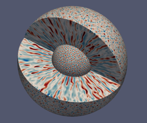
We first focus on a series of three simulations to highlight the specificities of fingering convection in global spherical geometry. Figure 3 provides three-dimensional renderings of the fingers, along with the corresponding kinetic energy spectra, of three cases that share $R_\rho = 1.1$, $Pr = 7$ and $Le = 3$ and differ by $Ra_\xi$, which increases from $10^8$ to $2\times 10^{10}$ (simulations 123, 118 and 103 in table 3). The convective power injected in the fluid is accordingly multiplied by $500$ between the simulation closest to onset, illustrated in figure 3(a), and the most supercritical one, shown in figure 3(c). For the least forced simulation (figure 3a), the flow is dominated by coherent radial filaments that extend over the entire spherical shell. These particular structures are reminiscent of the ‘elevator modes’ found in periodic planar models (e.g. Radko Reference Radko2013, § 2.1). Inside each of these filaments $T$, $\xi$ and $u_r$ can be considered to be quasi-uniform. The velocity field reaches relatively small amplitudes, with a poloidal Reynolds number $Re_{pol} \approx 10$. Geometrical patterns link the fingers together over spherical surfaces, and it appears that fingers emerge at the vertices of polygons in the vicinity of the inner sphere. Fingers have an almost constant width in the bulk of the domain. The rather large polygonal patterns that appear on the outer surface of the three-dimensional rendering are due to the weakening of the radial velocity in the vicinity of the outer boundary layer, that goes along with a widening of the finger as it penetrates the boundary layer. The spectrum of this simulation, displayed in figure 3(d), presents a marked maximum, with an average spherical harmonic degree $\ell _h$ (recall (2.21)) of $39$. The majority of the poloidal kinetic energy of the fluid is stored in degrees close to this peak. The quasi-homogeneous lateral thickness of fingers in figure 3(a) illustrates this spectral concentration.

Figure 3. (a–c) Three-dimensional renderings of the radial velocity for three simulations carried out using $R_\rho = 1.1$, $Pr = 7$ and $Le = 3$, and $Ra_\xi =10^8, 10^9$ and $2\times 10^{10}$ (simulations 123, 118 and 103 in table 3), for (a), (b) and (c), respectively. Inner and outer spherical surfaces correspond to $r_i + 0.03$ and $r_o - 0.04$, respectively. (d) Poloidal kinetic energy spectra as a function of spherical harmonic degree $\ell$ for these three simulations. Dashed vertical lines correspond to the average spherical harmonic degree $\ell _h$ (see (2.21)), of value $39$, $75$ and $166$, for $Ra_\xi =10^8, 10^9$ and $2\times 10^{10}$.

Figure 3(b) reveals that a strengthening of the forcing leads to an increase of the magnitude of the velocity, with $Re_{pol} = 28$, alongside a gradual loss of the coherent tubular structure of the fingers in favour of undulations and occasional branchings. They contract horizontally, leading to a shift of $\ell _h$ to a higher value of $75$. The geometrical patterns remain well defined over the inner sphere but appear attenuated at the outer spherical surface, again the signature of the effect of the outer boundary layer. Further increase of the injected convective power causes the occasional fracture of fingers in the radial direction, see figure 3(c), as they assume the shape of flagella reminiscent of the modes of Holyer (Reference Holyer1984, figure 1). Although the fingers gradually lose their vertical coherence with increased convective forcings, they still present an anisotropic elongated structure in the radial direction. Accordingly, the lateral thickness of the fingers continues to decrease and $\ell _h$ now reaches a value of $166$. That amounts to finding $O(10^4)$ such elongated structures at any radius $r$ in the bulk of the flow.

3.2. Mean profiles and compositional boundary layers

We now assess the impact of fingers on the average temperature and composition profiles within the spherical shell. Figure 4(a,b) shows the time-averaged radial profiles of temperature and composition of four simulations that share $|Ra_T| =3.66 \times 10^9$, $Pr = 7$, $Le = 3$ and differ by the prescribed $Ra_\xi$, whose value goes from $4.392 \times 10^9$ to $1.1 \times 10^{10}$, with a concomitant decrease of $r_\rho$ from $0.75$ down to $5 \times 10^{-4}$.

Figure 4. (a) Time-averaged radial profile of temperature, $\varTheta$, for four simulations sharing $|Ra_T| = 3.66 \times 10^{9}$, $Pr = 7$ and $Le = 3$, and increasing values of $r_\rho$ (simulations 106, 110, 112 and 113 in table 3). (b) Time-averaged radial profile of composition, $\varXi$, for the same simulations. The inset shows a magnification of the inner boundary layer, whose edge is shown with a thick vertical segment. In both panels, the dashed lines correspond to the diffusive reference profile.

The increase of $Ra_\xi$ impacts composition more than temperature, as it leads to steeper boundary layers and flatter bulk profiles of $\xi$ that substantially deviate from their diffusive reference, displayed with a dashed line in figure 4(b). Inspection of figure 4(a) shows that this trend exists but is less marked for temperature. Accordingly, the bulk temperature and composition drops, $\varDelta _b \varTheta$ and $\varDelta _b \varXi$, introduced above decrease as $Ra_\xi$ increases, in a much more noticeable manner for composition than for temperature. Boundary layer asymmetry inherent in curvilinear geometries (Jarvis Reference Jarvis1993) is clearer with increasing $Ra_\xi$: for the largest forcing considered here, approximately $40\,\%$ ($10\,\%$) of the contrast of composition is accommodated at the inner (outer) boundary layer.

To enable comparison with results from unbounded studies, we seek scaling laws for the effective contrasts $\varDelta _b \varTheta$ and $\varDelta _b \varXi$ that develop in the fluid bulk. To that end, and in line with the characterisation of boundary layers we introduced above, we first make use of the heat and composition flux conservation over spherical surfaces. Assuming that temperature and composition vary linearly within boundary layers yields

(3.1a,b)\begin{equation} \left(\dfrac{r_i}{r_o}\right)^2 \dfrac{\varDelta_i \varTheta}{\varDelta_o \varTheta} = \dfrac{\lambda_i}{\lambda_o}, \quad \left(\dfrac{r_i}{r_o}\right)^2 \dfrac{\varDelta_i \varXi}{\varDelta_o \varXi} = \dfrac{\lambda_i}{\lambda_o} , \end{equation}

where the $r_i/r_o$ factors emphasise the asymmetry of the boundary layer properties caused by the spherical geometry. To derive scaling laws for the ratio of the temperature and composition drops at both boundary layers, one must invoke a second hypothesis. In classical Rayleigh–Bénard convection in an annulus, Jarvis (Reference Jarvis1993) made the additional assumption that the boundary layers are marginally unstable (Malkus Reference Malkus1954). In other words, a local Rayleigh number defined on the boundary layer thickness should be close to the critical value to trigger convection. Later numerical simulations in three dimensions by Deschamps, Tackley & Nakagawa (Reference Deschamps, Tackley and Nakagawa2010) in the context of infinite Prandtl number convection and by Gastine et al. (Reference Gastine, Wicht and Aurnou2015) for $Pr=1$, however, showed that this hypothesis failed to correctly account for the actual boundary layer asymmetry observed in spherical geometry. For fingering convection in bounded domains, Radko & Stern (Reference Radko and Stern2000) nonetheless showed that the marginal stability argument provides a reasonable description of the boundary layers for composition. We here test this hypothesis by introducing the local thermohaline Rayleigh numbers $Ra^{\lambda _i}$ and $Ra^{\lambda _o}$ defined over the extent of the inner and outer boundary layers

(3.2a,b)\begin{align} Ra^{\lambda_{i}} = g_{i} \lambda_{i}^3 \left( Ra_\xi \varDelta_i \varXi - |Ra_T| \varDelta_i \varTheta \right), \quad Ra^{\lambda_{o}} = g_{o} \lambda_{o}^3 \left( Ra_\xi \varDelta_o \varXi - |Ra_T| \varDelta_o \varTheta \right), \end{align}

where $g_i$ and $g_o$ denote the acceleration due to gravity at the inner and outer boundaries, with $g_i/g_o = r_i/r_o$. We note in passing that gravity increasing linearly with radius is the second factor responsible for the boundary layer asymmetry. Equating $Ra^{\lambda _{i}}$ and $Ra^{\lambda _{o}}$ to a critical value $Ra^c$ gives, in light of (3.1a,b),

(3.3)\begin{equation} \left(\dfrac{\lambda_i}{\lambda_o}\right)^3 = \dfrac{r_o}{r_i} \dfrac{\varDelta_o \varXi}{\varDelta_i \varXi}. \end{equation}

Further use of (3.1a,b) yields

(3.4)\begin{equation} \dfrac{\lambda_o}{\lambda_i} = \left(\dfrac{r_i}{r_o}\right)^{-1/4}, \end{equation}

and

(3.5)\begin{equation} \dfrac{\varDelta_o \varXi}{\varDelta_i \varXi} = \left(\dfrac{r_i}{r_o}\right)^{7/4} , \end{equation}

both of which are a function of the sole radius ratio $r_i/r_o$.

Figure 5 shows the conformity of these two laws to the numerical dataset, which has a constant radius ratio $r_i/r_o=0.35$. In figure 5(a), we observe a close to linear increase of $\lambda _o$ with $\lambda _i$ over two orders of magnitude of variations. A least-squares fit performed for those simulations with $\lambda _i < 0.02$ provides $\lambda _o=1.18\,\lambda _i$ instead of the expected $\lambda _o=1.30\,\lambda _i$ from (3.4). Simulations causing this departure are those close to onset with thick boundary layers within which the linearity assumption may not hold. Likewise, we see in figure 5(b) that (3.5) captures the relative ratio $\varDelta _o \varXi /\varDelta _i \varXi$ within the dataset. We find $\varDelta _o \varXi = 0.14 \varDelta _i \varXi$ instead of the predicted $\varDelta _o \varXi = 0.16 \varDelta _i \varXi$, and note that the dispersion about a linear law is maximum for strongly driven simulations (those with smaller $r_\rho$ in figure 5b). These results indicate that, in contrast with Rayleigh–Bénard convection, the marginal stability hypothesis provides a good way to characterise the boundary layer asymmetry in spherical-shell fingering convection, with the caveat that confirmation of this finding should be sought for radius ratios other than the one considered in this study.

Figure 5. (a) Thickness of the outer boundary layer, $\lambda _o$, as a function of the thickness of the inner boundary layer, $\lambda _i$. (b) Composition contrast across the outer boundary layer, $\varDelta _o \varXi$, as a function of its inner counterpart, $\varDelta _i \varXi$. In both panels, the dashed lines correspond to a linear fit to data retaining only those simulations with $\lambda _i < 0.02$.

In order to obtain a relationship between the contrasts across the bulk, $\varDelta _b \varXi$ and $\varDelta _b \varTheta$, recall that the Sherwood and Nusselt numbers $Sh$ and $Nu$ are expected to read at $r=r_o$

(3.6a,b)\begin{equation} Sh = \dfrac{r_o}{r_i} \dfrac{\varDelta_o \varXi}{\lambda_o}, \quad Nu = \dfrac{r_o}{r_i} \dfrac{\varDelta_o \varTheta}{\lambda_o}, \end{equation}

if the linearity assumption for composition and temperature holds within the chemical boundary layer. Combining these definitions with (2.22a–c) and (3.4)–(3.5) yields the following relationship between $\varDelta _b \varTheta$, $\varDelta _b \varXi$, $Nu$ and $Sh$:

(3.7)\begin{equation} \dfrac{1 - \varDelta_b \varXi}{1 - \varDelta_b \varTheta} = \dfrac{Sh}{Nu}. \end{equation}

Figure 6(a) shows that there is convincing evidence for a linear relationship between $(1 - \varDelta _b \varXi )/(1 - \varDelta _b \varTheta )$ and $Sh/Nu$ across the parameter space sampled by the dataset; the slope is equal to $0.84$ instead of the expected value of one. This might come from the uncertainty related to the departure from the linearity assumption for the chemical boundary layer, possibly leading to underestimation of the true value of the Sherwood number.

Figure 6. (a) Value of $(1 - \varDelta _b \varXi )/(1 - \varDelta _b \varTheta)$ as a function of $Sh/Nu$. (b) Thickness of the inner boundary layer as a function of $Pe^{-1/3}\mathcal {L}_{h}^{2/3}$ derived in (3.12). In each panel, the result of the linear regression is shown with a dashed line.

For a better understanding of (3.7), it is insightful to split the mean radial profiles into the sum of a reference conducting state and fluctuations denoted by primed quantities

(3.8a,b)\begin{equation} \varXi=\xi_c+\varXi',\quad \varTheta=T_c+\varTheta'. \end{equation}

Using the definition of the flux ratio (2.19), (3.7) can be rewritten as

(3.9)\begin{equation} \dfrac{\varDelta_b \varXi'}{\varDelta_b \varTheta'} \approx R_\rho Le\gamma^{-1}, \end{equation}

where we have assumed that $\varDelta _b \xi _c = \varDelta _b T_c \approx 1$.

Following Yang et al. (Reference Yang, van der Poel, Ostilla-Mónico, Sun, Verzicco, Grossmann and Lohse2015), we now evaluate whether results coming from classical Rayleigh–Bénard convection models regarding the nature of the boundary layers are still applicable to bounded double-diffusive convection. In that regard, the cornerstone of the GL theory is that the kinetic and thermal boundary layer thicknesses adhere to the Prandtl–Blasius model (e.g. Schlichting & Gersten Reference Schlichting and Gersten2018, § 9.2). In this model, the boundary layer corresponds to a laminar flow over a horizontal plate and the temperature and chemical composition are treated as passive scalars. For fingering convection with $Le>1$, this translates to

(3.10a,b)\begin{equation} \dfrac{\lambda_\xi}{\mathcal{L}_{h}} \sim Sc^{-1/2}\,Re_h^{-1/2} (Sc < 1), \quad \dfrac{\lambda_\xi}{\mathcal{L}_{h}} \sim Sc^{-1/3}\,Re_h^{-1/2} (Sc > 1), \end{equation}

where $\lambda _\xi$ denotes the thickness of the inner or outer chemical boundary layer, and $Re_h = u_h \mathcal {L}_{h}/\nu$ is a Reynolds number defined using the length scale $\mathcal {L}_{h}$ and the near-boundary horizontal flow velocity $u_h$. For tubular fingers, mass conservation between the finger core of typical diameter $\lambda _\xi$ (Yang et al. Reference Yang, Verzicco and Lohse2016, their figure 10) and the horizontal flows that converge towards the finger in the boundary layers demands

(3.11a,b)\begin{equation} u_h \lambda_\xi {\rm \pi}\mathcal{L}_{h} \approx u_r \dfrac{\rm \pi}{4} \lambda_\xi^2\ (Sc < 1),\quad \dfrac{\lambda_\xi}{\lambda_U}u_h \lambda {\rm \pi}\mathcal{L}_{h} \approx u_r \dfrac{\rm \pi}{4} \lambda_\xi^2\ (Sc > 1) , \end{equation}

where $\lambda _U$ denotes the thickness of the velocity boundary layer. The factor $\lambda _\xi /\lambda _U$ in the equation on the right reflects the fact that the velocity boundary layer is nested in the compositional one when $Sc > 1$. As such, and assuming linear boundary layers, the relevant horizontal flow velocity has to be rescaled by the relative thickness of both boundary layers. Using (3.10a,b), this then leads to the unique form

(3.12)\begin{equation} \lambda_\xi \sim Pe^{-1/3}{\mathcal{L}_{h}}^{2/3}, \end{equation}

for both Schmidt number end members. Figure 6(b) shows the thickness of the inner compositional boundary layer ($\lambda _\xi = \lambda _i$) as a function of this theoretical scaling for all the simulations where the boundary layers could be evaluated. The reduced scatter of the data as well as the slope of the best fit power law being close to one indicate an excellent agreement with the Prandtl–Blasius model combined with the hypothesis of tubular fingers.

3.3. Effective density ratio

In order to compare the dynamics with unbounded domains, the common practice in bounded planar geometry (Schmitt Reference Schmitt1979b; Radko & Stern Reference Radko and Stern2000; Yang et al. Reference Yang, Chen, Verzicco and Lohse2020) consists in introducing an effective density ratio within the bulk of the domain expressed by

(3.13)\begin{equation} R_\rho^\star= R_\rho \dfrac{\varDelta_b \varTheta}{\varDelta_b \varXi}. \end{equation}

This measure is appropriate to fingering convection in Cartesian domains with $R_\rho \ll Le$, given the piecewise-linear nature of the composition profile (see e.g. figure 2 of Yang Reference Yang2020). This estimate is, however, not suitable close to onset as the boundary layer definition becomes ill posed. An extra complication arises in spherical geometry since our definition of boundary layers only retains the linear part of the drop of composition, which tends to overestimate $\varDelta _b \varXi$ (recall figure 2 and the discussion in § 2.5). As such, it appears more reliable to introduce an effective density ratio (and its normalised counterpart) based on the gradients of temperature and composition at mid-depth

(3.14a,b)\begin{equation} R_\rho^\star=-R_\rho \left. \dfrac{\mathrm{d} \varTheta}{\mathrm{d}r}\right|_{r_m} \left(\left.\dfrac{\mathrm{d} \varXi}{\mathrm{d}r}\right|_{r_m}\right)^{-1},\quad r_\rho^\star= \dfrac{R_\rho^\star- 1}{Le -1}. \end{equation}

We saw above that the contrast of composition across the bulk (or fingering region) is systematically lower than that of temperature. It hence follows that $R_\rho ^\star > R_\rho$ and $r_\rho ^\star > r_\rho$.

3.4. Finger width

We now derive scaling laws for fingering convection based on our $123$ bounded simulations, beginning with the typical lateral extent $\mathcal {L}_{h}$ of a finger, as defined in (2.21). In his seminal contribution, Stern (Reference Stern1960) predicts a scaling of the form

(3.15)\begin{equation} \mathcal{L}_{h} \propto |Ra_T|^{-1/4}, \end{equation}

for an unbounded Boussinesq fluid subjected to uniform thermal and chemical background gradients when $Le \gg R_\rho \gg 1$. A least-squares fit of our dataset yields

(3.16)\begin{equation} \mathcal{L}_{h} = 4.23\,|Ra_T|^{-0.23}, \end{equation}

where the exponent found is rather close to the expected value of $-0.25$, for values of $|Ra_T|$ spanning $6$ orders of magnitude. Yet, inspection of figure 7(a) reveals that this scaling fails to capture a second dependency to $r_\rho$. At a given value of $|Ra_T|$, we observe indeed that $\mathcal {L}_{h}$ is an increasing function of $r_\rho$. In order to make progress, let us assume that the finger width is controlled by a balance between buoyancy and viscous forces. In addition, we resort to the tall finger hypothesis introduced by Stern (Reference Stern1975, p. 192) and christened by Smyth & Kimura (Reference Smyth and Kimura2007), which consists of neglecting along-finger derivatives in favour of cross-finger derivatives. Accordingly, the time and volume average of the radial component of (2.3) becomes

(3.17)\begin{equation} \overline{\left\langle \left(-\dfrac{Ra_T}{Pr}T + \dfrac{Ra_\xi}{LePr} \xi\right) \dfrac{r}{r_o} \right\rangle_{V}} \sim \overline{\left\langle \nabla^2 \boldsymbol{u} \boldsymbol{\cdot}\boldsymbol{e}_r \right\rangle_{V}} \sim \dfrac{Re_{pol}}{\mathcal{L}_{h}^2}. \end{equation}

Likewise, the average of the heat equation (2.4) leads to

(3.18)\begin{equation} Re_{pol} \dfrac{\varDelta_b \varTheta}{\lambda_b} \sim \dfrac{\overline{\left\langle T \right\rangle_{V}}}{Pr\mathcal{L}_{h}^2}. \end{equation}

Finally, a relationship between $\overline {\left \langle T \right \rangle _{V}}$ and $\overline {\left \langle \xi \right \rangle _{V}}$ is expressed by means of the flux ratio $\gamma$

(3.19)\begin{equation} \overline{\left\langle \xi \right\rangle_{V}} \sim \dfrac{Le|Ra_T|}{\gamma Ra_\xi} \overline{\left\langle T \right\rangle_{V}}, \end{equation}

which, in light of (2.19), assumes implicitly that the radial velocity correlates well with thermal and chemical fluctuations. Upon combining (3.17)–(3.19), we obtain

(3.20)\begin{equation} \mathcal{L}_{h}^{-4} \sim (\gamma^{-1}-1) |Ra_T| \dfrac{\varDelta_b \varTheta}{\lambda_b}. \end{equation}

The bulk temperature gradient $\varDelta _b \varTheta /\lambda _b$ aside, this expression is equivalent to that proposed by Taylor & Bucens (Reference Taylor and Bucens1989) in the discussion of their experimental results. Figure 7(b) shows $\mathcal {L}_{h}$ as a function of $|Ra_T|(\gamma ^{-1}-1)$. The extra factor $(\gamma ^{-1}-1)$ removes the dispersion observed in figure 7(a). A least-squares fit of $\log _{10}(\mathcal {L}_{h})$ vs $\log _{10}[|Ra_T|(\gamma ^{-1}-1)]$ leads to

(3.21)\begin{equation} \mathcal{L}_{h} = 5.28\left[(\gamma^{-1} -1)|Ra_T|\right]^{-0.26}. \end{equation}

The exponent of $|Ra_T|$ remains close to the value of $-0.25$ proposed by Stern (Reference Stern1960). In order to assess the effect of the $\varDelta _b \varTheta /\lambda _b$ term, we introduce the misfit

(3.22)\begin{equation} \chi_y^2 = \sqrt{\dfrac{1}{N} \sum_{i = 1}^N \left|\dfrac{\tilde{y}_i - y_i}{y_i}\right|^2}, \end{equation}

where $N$ is the number of simulations, $y_i$ is the $i$th measured value of $\log _{10}(\mathcal {L}_{h})$ and $\tilde {y}_i$ its prediction by the least-squares fit of interest. In the absence of a correction factor, recall (3.16), we obtain $\chi _y^2=0.091$. With the full correction (3.20), $\chi _y^2=0.023$, which amounts to a fourfold reduction. The misfit increases by a modest amount to $0.025$ if we omit the factor $\varDelta _b \varTheta /\lambda _b$ in (3.20). It thus appears reasonable to ignore that factor for the sake of parsimony. In the remainder of this study, we will therefore adhere to

(3.23)\begin{equation} \mathcal{L}_{h}^4 \sim \dfrac{\gamma}{1 - \gamma} |Ra_T|^{-1}. \end{equation}

Figure 7. (a) Horizontal length scale $\mathcal {L}_h$ (2.21) as a function of $|Ra_T|$. (b) Value of $\mathcal {L}_h$ as a function of $|Ra_T|(\gamma ^{-1}-1)$. In both panels, the dashed lines correspond to power law fits.

Following the idea of Schmitt (Reference Schmitt1979b), we now examine whether the average spherical harmonic degree $\ell _h$ of fingers in developed convection relates to the degree of the fastest growing mode, $\ell _{FG}$. Linearisation of the system (2.2)–(2.5) is conducted by considering small perturbations of the poloidal scalar $W$, temperature $T$ and composition $\xi$. Performing a spherical harmonic expansion of these variables leads to equations decoupled in harmonic degree $\ell$ and independent of the spherical harmonic order $m$. We use the ansatz

(3.24)\begin{equation} [W_\ell, T_\ell, \xi_\ell](t, r) = [\widehat{W_\ell}, \widehat{T_\ell}, \widehat{\xi_\ell}](r) \exp\left(\tau_\ell t\right), \end{equation}

where $[\widehat {W_\ell }, \widehat {T_\ell }, \widehat {\xi _\ell }]$ are the radial shape functions of the perturbation of degree $\ell$. Focusing on the real-valued eigenvalues $\tau _\ell$ relevant to the fingering instability, we obtain the generalised eigenvalue problem

(3.25)\begin{equation} \mathcal{A}_\ell \boldsymbol{X}_\ell = \tau_\ell \mathcal{B}_\ell \boldsymbol{X}_\ell, \end{equation}

where $\mathcal {A}_\ell$ and $\mathcal {B}_\ell$ are real dense matrices, $\boldsymbol {X}_\ell \equiv [W_\ell, T_\ell, \xi _\ell ]^{\rm T}$ is the state vector and we understand that each eigenvalue depends on $\ell$, $Ra_T$, $Ra_\xi$, $Pr$ and $Le$. We resort to the Linear Solver Builder (LSB) package developed by Valdettaro et al. (Reference Valdettaro, Rieutord, Braconnier and Frayssé2007) to determine the harmonic degree $\ell _{FG}$ of the fastest growing mode which corresponds to $\ell _{FG} = {\rm arg\,max}_\ell \tau _\ell$ for any given set-up of the numerical dataset.

Figure 8(a) shows $\ell _{h}$ as a function of $\ell _{FG}$. To first order, $\ell _{h}$ grows almost linearly with $\ell _{FG}$ and the proportionality coefficient linking the two harmonic degrees seems to weakly depend on the input parameters. We find that $\ell _{h}$ is consistently greater than $\ell _{FG}$. The linear fit $\ell _{h} = 1.89\,\ell _{FG}$ is shown as a dashed line in figure 8(a), and is overall in agreement with the simulations. Significant departures occur for $\ell _{FG} < 30$, as the least turbulent simulations tend towards verifying $\ell _{h} = \ell _{FG}$ (see e.g. the pentagon at the bottom left of figure 8a). Far from onset, a large number of modes are excited and the broadening of the spectra noticeable in figure 3(d) reflects the nonlinear interaction of theses modes.

Figure 8. (a) Mean spherical harmonic degree $\ell _{h}$ as a function of the degree of the fastest growing mode $\ell _{FG}$; the dashed line shows the result of the linear regression. (b) Most linearly unstable degree $\ell _{FG}|Ra_T|^{-1/4}$ as a function of the supercriticality parameter $\epsilon$. The dashed line in panel (a) corresponds to a linear fit forced over the entire dataset, yielding a prefactor equal to $1.89$, while the best fit in panel (b) was obtained from the simulations with $\epsilon < 0.5$.

The fastest growing modes can be expanded in powers of a supercriticality parameter $\epsilon$ which quantifies the distance to onset of fingering convection

(3.26)\begin{equation} \epsilon = \dfrac{Ra_\xi-|Ra_T|}{|Ra_T|}=\dfrac{Le}{R_\rho}-1. \end{equation}

For finite Prandtl numbers, the first-order contribution reads (e.g. Schmitt Reference Schmitt1979b; Stern & Radko Reference Stern and Radko1998; Radko Reference Radko2010)

(3.27)\begin{equation} \ell_{FG}^4 \sim \epsilon |Ra_T|, \end{equation}

in the limit of vanishing $\epsilon$. Figure 8(b) shows the spherical harmonic degree of the fastest growing mode $\ell _{FG} |Ra_T|^{-1/4}$ as a function of the distance to onset $\epsilon$. The best fit to the data reveals a good agreement with the expected theoretical scaling whenever $\epsilon \ll 1$. Significant departures appear beyond $\epsilon \approx 0.5$, indicating the limit of validity of the scaling (3.27).

We hence retain from figure 8 that the hypothesis put forward by Schmitt (Reference Schmitt1979b) – i.e. that the finger width relates to the horizontal size of the fastest growing mode – works better for weakly nonlinear models, i.e. when $\epsilon \ll 1$. This observation will later be used to derive scaling laws for weakly nonlinear fingering convection.

3.5. Scaling laws for transport

We now aim at deriving integral scaling laws for the transport of composition and heat, and for the mean vertical velocity.

Figure 9(a) shows $Sh$ as a function of $Ra_\xi$, and two trends emerge: first, at any given $Ra_\xi$, numerical models with $r_\rho < 0.2$ (dark blue symbols) provide an effective upper bound for the transport of chemical composition. This upper bound of the Sherwood number $Sh$ grows with $Ra_\xi$ according to a power law that appears almost independent of $Pr$. Second, close to onset ($r_\rho \simeq 1$), simulations are organised along branches representative of a dependency of $Sh$ on $Ra_\xi$ much steeper than the one of the effective upper bound. Each branch corresponds to fixed values of $Ra_T$, $Pr$, and $Le$, and gradually tapers off to the $r_\rho \ll 1$ trend as the value of $r_\rho$ decreases along the branch. This prompts us to analyse the regimes $r_\rho \simeq 1$ and $r_\rho \ll 1$ separately.

Figure 9. (a) Sherwood number $Sh$ as a function of $Ra_\xi$. (b) Flux ratio $\gamma$ as a function of $R_\rho ^\star /Le$. The dashed line corresponds to the first bisector $\gamma =R_\rho ^\star /Le$.

It is also informative to inspect the variations of the turbulent flux ratio $\gamma$, as defined by (2.19), in both limits. Figure 9(b) shows $\gamma$ against $R_\rho ^\star /Le$. When $r_\rho \ll 1$, $\gamma$ substantially deviates from $R_\rho ^\star /Le$ and gradually saturates around values which decrease upon increasing the Lewis number: simulations with $Le=3, Pr=7$ (circles) saturate at $\gamma \approx 0.8$, while those with $Pr\leq 1$ (pentagons, hexagons, squares and triangles) gradually tapper off around values of $0.6$ and $0.4$ for $Le=10$ and $Le \geq 30$, respectively. The series of simulations with $Pr =7$ (circles) seems to suggest that the $\gamma \approx 0.8$ plateau may actually precede an increase at even lower values of $R_\rho ^\star /Le$, a trend predicted by Kunze (Reference Kunze1987) in the limit of $Pr, Le \gg 1$. In contrast, close to onset, the flux ratio is well described by $R_\rho ^\star /Le$

(3.28)\begin{equation} \gamma \approx \dfrac{R_\rho^\star}{Le}, \end{equation}

a behaviour consistent with the arguments put forward by Schmitt (Reference Schmitt1979b).

3.5.1. The $r_\rho \simeq 1$ regime

We shall start our analysis by investigating the weakly nonlinear regime characterised by small values of the supercriticality parameter $\epsilon$ defined above in (3.26). In the limit where $\gamma \approx R_\rho ^\star /Le$, the scaling law obtained for the finger width (3.20) can be rewritten by breaking down the mean radial profiles into a sum of the conducting state and fluctuations. This yields

(3.29)\begin{equation} \mathcal{L}_{h}^{-4} \sim |Ra_T|\left[\dfrac{Le}{R_\rho}\left(1+\dfrac{\varDelta_b \varXi'} {\lambda_b }\right)-1-\dfrac{\varDelta_b \varTheta'}{\lambda_b}\right], \end{equation}

where we have assumed that $|\mathrm {d}\xi _c /\mathrm {d} r| = \mathrm {d} T_c /\mathrm {d} r \approx 1$. Now, based on our previous findings that the finger width is well accounted for by the horizontal size of the fastest growing mode whenever $\epsilon \ll 1$ (recall figure 8), we have

(3.30)\begin{equation} |Ra_T|\left[\dfrac{Le}{R_\rho}\left(1+\dfrac{\varDelta_b \varXi'} {\lambda_b }\right)-1-\dfrac{\varDelta_b \varTheta'}{\lambda_b}\right] \sim |Ra_T|\left(\dfrac{Le}{R_\rho}-1\right), \end{equation}

which leads to

(3.31)\begin{equation} \dfrac{\varDelta_b \varTheta'}{\lambda_b} \sim \dfrac{\epsilon}{Le^2 \gamma^{-1}-1}, \end{equation}

in which the ratio of $\varDelta _b \varXi '/\varDelta _b \varTheta '$ has been estimated using (3.9).

Making use of the definitions (2.22a–c) then allows us to relate the ratio $\varDelta _b \varTheta '/\lambda _b$ to its boundary layer counterpart, namely

(3.32)\begin{equation} \dfrac{\varDelta_b \varTheta'}{\lambda_b} = \dfrac{\varDelta_o \varTheta'}{\lambda_o}\dfrac{\lambda_o+\lambda_i(\varDelta_i \varTheta'/\varDelta_o \varTheta')}{1-\lambda_i- \lambda_o } \approx \dfrac{\varDelta_o \varTheta'}{\lambda_o} \lambda_o[1+(r_i/r_o)^{-3/2}], \end{equation}

where the latter equality has been derived using our previous findings regarding the boundary layer asymmetry (3.4)–(3.5). Noting that $Nu-1\approx (r_o/r_i) \varDelta _o \varTheta '/\lambda _o$ and substituting the above expression in (3.31) yields

(3.33)\begin{equation} Nu - 1 \sim f(r_i/r_o)\lambda_o^{-1} \dfrac{\epsilon}{Le^2\gamma^{-1}-1}, \end{equation}

where $f(r_i/r_o) = (r_i/r_o)^{-1}[1+(r_i/r_o)^{-3/2}]^{-1}$ accounts for the dependence on the radius ratio $r_i/r_o$ inherent in the spherical-shell geometry. Beside these geometrical factors, this expression is strictly equivalent to (5.10) derived by Radko & Stern (Reference Radko and Stern2000) in bounded Cartesian domains under the assumption of tall laminar fingers in the fluid bulk.

The end of the derivation, however, differs from Radko & Stern (Reference Radko and Stern2000), in that they consider a boundary layer model where the buoyancy term is retained, while we have shown earlier that the compositional boundary layers rather adhere to the Prandtl–Blasius model (see (3.12) and figure 6).

To eliminate the Péclet number $Pe$ in (3.12), one can simply assume that viscous dissipation is well approximated by $D_\nu \sim (Re_{pol}/\mathcal {L}_{h})^2$. The power balance (2.17) (see also Appendix B) then directly yields

(3.34)\begin{equation} Pe \sim \mathcal{L}_{h} |Ra_T|^{1/2} Le (Nu -1)^{1/2} (\gamma^{-1}-1)^{1/2}. \end{equation}

Hence, combining (3.12), (3.33) and (3.34), the scaling relation for $Nu-1$ reads

(3.35)\begin{equation} Nu-1 \sim \dfrac{\epsilon^{6/5}|Ra_T|^{3/10}Le^{2/5}(\gamma^{-1}-1)^{3/10}}{ (\gamma^{-1}Le^2-1)^{6/5}}, \end{equation}

where the order-one geometrical factors have been omitted. To end up with a scaling relation which solely depends on control quantities, one can further approximate the flux ratio by $\gamma \approx R_\rho /Le$, or equivalently assume that $\gamma ^{-1}-1 \approx \epsilon$. Noting that this latter assumption is more restrictive than (3.28) and that $R_\rho /Le=1-\epsilon$, the first-order contribution leads to

(3.36)\begin{equation} Nu-1 \sim \epsilon^{3/2}|Ra_T|^{3/10}Le^{-2}, \end{equation}

while the corresponding scaling behaviour for $Sh-1$ then reads

(3.37)\begin{equation} Sh-1\approx Le^2 (Nu-1) \sim \epsilon^{3/2}|Ra_T|^{3/10}. \end{equation}

The scaling for the vertical velocity (3.34) then becomes

(3.38)\begin{equation} Pe \sim \epsilon |Ra_T|^{2/5}\,. \end{equation}

Equations (3.36)–(3.38) form the weakly nonlinear scaling behaviour for bounded fingering convection. The scaling exponents on the supercriticality parameter $\epsilon$ differ from those derived by Radko & Stern (Reference Radko and Stern2000) due to different boundary layer models. Figure 10 shows an evaluation of these predictive scaling laws for the $47$ simulations with $\epsilon < 1$. Among those, the $25$ simulations with $Pr \geq 1$ are reasonably well accounted for by the weakly nonlinear laws. Best fits using the $22$ simulations with $\epsilon < 0.5$ yield scaling exponents of $\approx 1.1$ for the heat and composition transport, moderately larger than the expected slope of one, while the vertical velocity follows an exponent closer to unity. In contrast, the remaining $22$ simulations with $Pr < 1$ are more scattered, they significantly depart from the asymptotic laws and seem to demand an extra dependence on the Prandtl number. This is particularly obvious for the scaling of the Sherwood number shown in figure 10(b).

Figure 10. (a) Vertical convective transport of heat $Nu-1$ as a function of the theoretical weakly nonlinear scaling (3.36) for all the simulations with $\epsilon < 1$. (b) Vertical convective transport of composition as a function of the scaling (3.37). (c) Convective velocity as a function of the scaling (3.38). The dashed lines correspond to the best fits obtained for the numerical simulations with $Pr \geq 1$ and $\epsilon < 0.5$.

The previous derivation rests on several assumptions that become questionable in the limit of small Prandtl numbers. Among the most likely shortcomings, one can think of: (i) the approximation of the flux ratio by $\gamma \approx R_\rho /Le$ getting more uncertain on decreasing $Pr$; (ii) the relation between the finger width and the size of the fastest growing mode breaking down at low $Pr$ or involving a more intricate dependence on $\epsilon$ (Schmitt Reference Schmitt1979b; Radko Reference Radko2010); and (iii) inertia becoming sizeable, thus invalidating the laminar tall finger hypothesis. All in all, these additional hurdles hamper the derivation of predictive scaling laws for bounded domains that would hold in the small Prandtl number limit.

For the purpose of comparison with the local unbounded computations by Brown et al. (Reference Brown, Garaud and Stellmach2013) when $Pr < 1$, we nevertheless show in Appendix C that adjusted diagnostics which incorporate the modification of the background profiles into account can be described by simple polynomials fits on $Pr$ and $\epsilon ^\star /Le$, where $\epsilon ^\star =Le/R_\rho ^\star -1$.

3.5.2. The $r_\rho \ll 1$ regime

Turning our attention to the second limit, we retain arbitrarily those 41 simulations with $r_\rho < 0.1$, which cover all values of $Pr$ from $0.03$ to $7$.

Figure 11(a) shows $Sh-1$ versus $Ra_\xi$ for these simulations, alongside the $31$ bounded Cartesian simulations of Yang et al. (Reference Yang, Verzicco and Lohse2016) that satisfy $r_\rho > 0$. A least-squares fit of $Sh-1$ as a function of $Ra_\xi$ yields $Sh-1 \sim Ra_\xi ^{0.27}$ for our dataset and $Sh-1 \sim Ra_\xi ^{0.31}$ for that of Yang et al. (Reference Yang, Verzicco and Lohse2016). The extension of the theory of Grossmann & Lohse (Reference Grossmann and Lohse2000) for Rayleigh–Bénard convection to fingering convection by Yang et al. (Reference Yang, van der Poel, Ostilla-Mónico, Sun, Verzicco, Grossmann and Lohse2015) predicts $Sh \sim Ra_\xi ^{1/3}$ in the $Ra_\xi \gg 1$ limit when dissipation occurs in the fluid bulk. However, for the range of $Ra_\xi$ covered in this study, a non-negligible fraction of dissipation is expected to happen within the boundary layers. In addition, our mixture of Prandtl numbers above and below unity may result in superimposed transport regimes. As such, the smaller value of the scaling exponent, as well as the larger spread of the data, compared with those of Yang et al. (Reference Yang, Verzicco and Lohse2016) over a comparable range of $Ra_\xi$, are not surprising: Yang et al. (Reference Yang, Verzicco and Lohse2016) consider a single combination of parameters $(Pr=7,Le=100)$ that makes it possible to reach values of $r_\rho$ smaller than ours. We only retained the simulations by Yang et al. (Reference Yang, Verzicco and Lohse2016) that satisfied the criterion $r_\rho >0$, viz. $R_\rho >1$; yet fingers in their case remain stable down to $R_\rho \approx 0.1$, where the scaling $Sh-1 \sim Ra_\xi ^{0.31}$ still holds (not shown). Finally, we note that the chemical transport for the $Pr < 1$ data shown in figure 11(a) also follows the $Ra_\xi ^{0.27}$ law, in stark contrast to the predictions of a constant $Sh$ for a fixed $(Le, Pr)$ pair derived by Brown et al. (Reference Brown, Garaud and Stellmach2013) in unbounded planar models with $Pr\ll 1$.

Figure 11. (a) Value of $Sh-1$ as a function of $Ra_\xi$ for our numerical simulations with $r_\rho < 0.1$ alongside the data from Yang et al. (Reference Yang, Verzicco and Lohse2016) that fulfil $R_\rho > 1$. (b) Value of $Pe|Ra_T|^{1/4}$ as a function of $Ra_\xi$. In both panels, dashed and dotted lines correspond to least-square fits to our data and to those of Yang et al. (Reference Yang, Verzicco and Lohse2016), respectively.

Using (3.34), the definition of the flux ratio (2.19) and the scaling for $Sh-1$ with $Ra_\xi$ just discussed, and assuming that $[\gamma (1-\gamma )]^{1/2}$ can be considered constant, we expect

(3.39)\begin{equation} Pe \sim Ra_\xi^{2/3}|Ra_T|^{-1/4}, \end{equation}

in the asymptotic $Sh \sim Ra_\xi ^{1/3}$ regime. Figure 11(b) shows $Pe | Ra_T |^{1/4}$ as a function of $Ra_\xi$ for our dataset and that of Yang et al. (Reference Yang, Verzicco and Lohse2016). Least-squares fits yield scaling exponents that are remarkably close to $2/3$ for both subsets, and a spread of our data along the best-fit line less pronounced than in figure 11(a). The difference in the prefactors of the best-fit lines describing our dataset and that of Yang et al. (Reference Yang, Verzicco and Lohse2016) can be ascribed to the differences in model set-ups (Cartesian vs spherical geometry and constant gravity vs gravity increasing with $r$).

A few comments are in order with regard to (3.39): operating at fixed $Le=100$, Yang et al. (Reference Yang, Verzicco and Lohse2016) propose a scaling for the vertical velocity in terms of the Reynolds number $Re$

(3.40)\begin{equation} Re \propto R_\rho^{-1/4} Ra_\xi^{1/2} \propto Ra_\xi^{3/4} | Ra_T |^{-1/4} Le^{-1/4}, \end{equation}

which, in light of their figure 4(b), does not yield as good an agreement with their data as the scaling proposed here for $Pe$, and shown in figure 11(b). Expressing our proposed scaling in terms of $Re$ gives

(3.41)\begin{equation} Re \sim Ra_\xi^{2/3} | Ra_T |^{-1/4} Sc^{-1}, \end{equation}

which exhibits a slightly smaller dependency on $Ra_\xi$ than the one put forward by Yang et al. (Reference Yang, Verzicco and Lohse2016), and does a better job of fitting their data (not shown). Yang et al. (Reference Yang, Verzicco and Lohse2016) acknowledged that additional dependency on $Pr$ and $Sc$ (or $Le$) might occur since only one combination is considered in their study, in particular when discussing the scaling $Re \sim Ra_\xi | Ra_T |^{-1/2}$ proposed by Hage & Tilgner (Reference Hage and Tilgner2010) based on their experimental data with $Pr \approx 9$ and $Sc\approx 2200$. The exponents found by Hage & Tilgner (Reference Hage and Tilgner2010) are markedly different from the ones inferred from our analysis. It should be noted, however, that their experimental data cover a region of parameter space where the density ratio is mostly smaller than unity, in which fingers can be gradually replaced by large-scale convection. Under those circumstances, the hypothesis that dissipation can be expressed by $D_\nu \sim (Re_{pol}/\mathcal {L}_{h})^2$, with $\mathcal {L}_{h}$ the typical finger width, breaks down.

4.1. Flow morphology

Figure 12 shows 3-D renderings of snapshots of the azimuthal velocity for four selected numerical simulations. Upper panels (a,b) correspond to simulations which share the same parameters $Pr=0.3$, $|Ra_T|=10^8$, $Le=10$ and only differ in the values of the density ratio $R_\rho$, $R_\rho =6$ in figure 12(a) and $R_\rho =5$ in figure 12(b). To highlight the spatial distribution of the toroidal jet, figure 12(a,b) also shows streamlines of the large-scale component of the flow truncated at spherical harmonic degree $\ell =7$. In both simulations, the large-scale component of the flow takes the form of one single jet which reaches its maximum amplitude around mid-shell (red thick streamline tubes). We note in passing that the 22 simulations with $Pr<1$ of our dataset which develop toroidal jets systematically feature one singly oriented jet that spans most of the spherical-shell volume. The absence of background rotation precludes the existence of a preferential direction in the domain, and the axis of symmetry of the jet has the freedom to evolve over time. In panel (a), the toroidal Reynolds number reaches $24$, comparable to the velocity of the fingers $Re_{pol}=41$. The fivefold increase of the buoyancy power between figures 12(a) and 12(b) results in a stronger jet, which now reaches $Re_{tor}=87$, a value slightly larger than the finger velocity $Re_{pol}=77$. Interestingly, a further decrease of $R_\rho$ to $3.25$ (not shown) results in the decrease of $Re_{tor}$ and the eventual demise of toroidal jets for lower $R_\rho$. This is suggestive of a minimum threshold value of $R_\rho$ favourable to trigger jet formation.

Figure 12. Three-dimensional renderings of the instantaneous longitudinal velocity $u_\varphi$ for four simulations. The inner and outer spherical surfaces correspond to $r_i + 0.03$ and $r_o - 0.04$. (a,b) The two simulations share $Pr=0.3$, $Le=10$ and $Ra_T=-10^8$ (simulations 57 and 53 in table 3). The value of $R_\rho$ is equal to $6$ in (a) and $4$ in (b). Streamlines correspond to the large-scale component of the flow, truncated at a spherical harmonic degree $\ell = 7$. The width and the colour of the streamlines vary according to the local squared velocity. The two simulations on the bottom row (c,d) share $Pr=3$, $Le=10$ and $R_\rho =1.5$ (simulations 84 and 80). The simulation shown in (c) has $(Ra_T,Ra_\xi )=(-1.5 \times 10^9, 10^{10})$, while that shown in (d) has $(Ra_T,Ra_\xi )=(-7.5 \times 10^9, 5 \times 10^{10})$.

The numerical models shown in the lower panels (c,d) of figure 12 share the same values of $Pr=3$, $Le=10$ and $R_\rho =1.5$ but differ in their values of $Ra_\xi$ and $Ra_T$. In the case shown in figure 12(c) with $Ra_\xi =10^{10}$, faint multiple jets of alternated directions develop. Their amplitudes remain, however, weak compared with the finger velocity with $Re_{tor}=14$ and $Re_{pol}=72$. As can be seen in the equatorial plane (colatitude $\theta ={\rm \pi} /2$), jets do not exhibit a perfectly coherent concentric nature over the entire fluid volume but rather adopt a spiralling structure with significant amplitude variations. As shown in figure 12(d), an increase of the convective driving to $Ra_\xi = 5 \times 10^{10}$ goes along with the formation of a stack of $6$ alternated jets. Although their amplitude remains smaller than the fingering velocity ($Re_{tor}=45$ and $Re_{pol}=134$), toroidal jets now adopt a quasi-concentric structure with well-defined boundaries. This latter configuration is reminiscent of the simulations of Yang et al. (Reference Yang, Verzicco and Lohse2016), who also report the formation of multiple jets in local Cartesian numerical models with $Pr =7$ and $R_\rho =1.6$ when $Ra_\xi \geq 10^{11}$. Similarly to Yang et al. (Reference Yang, Verzicco and Lohse2016), we also observe that toroidal jets develop in configurations with $Pr \geq 1$ for small values of $R_\rho$ and sufficiently large values of $Ra_\xi$. Critical values of those parameters required to trigger jet formation are further discussed below.

4.2. Time evolution

To illustrate the growth of toroidal jets, we show in figure 13 the time evolution of the poloidal and toroidal kinetic energy alongside kinetic energy spectra for two illustrative numerical simulations which feature jets with $Ra_T = -10^8$, $Pr = 0.3$, $Le = 10$ and $R_\rho = 4$ (upper panels, simulation 53 in table 3) and $Ra_T = -1.5 \times 10^8$, $Pr = 1$, $Le = 10$ and $R_\rho = 1.3$ (lower panels, simulation 72). For the case with $Pr=0.3$ (figure 13a), $E_{{k}, {tor}}$ is initially $25$ times weaker than $E_{{k}, {pol}}$. Beyond $t\approx 4.2$, $E_{{k}, {tor}}$ grows exponentially over approximately one viscous diffusion time and saturates at a value which exceeds $E_{{k}, {pol}}$. In contrast, the case with $Pr=1$ (figure 13c) exhibits a much slower growth of the toroidal energy: $E_{{k}, {tor}}$ gains one order of magnitude in more than $3$ viscous diffusion times. At the saturation of the instability around $t\approx 9$, $E_{{k}, {tor}}$ remains a factor $3$ smaller than $E_{{k}, {pol}}$ in this case. The growth of the toroidal energy goes along with the formation of one or several large-scale jets (see figure 12), which are clearly visible in the kinetic energy spectra. Figures 13(b)–13(d) show the kinetic energy spectra as a function of the spherical harmonic degree at three different times: before the start of the instability (blue lines), during the exponential growth of the jets (yellow lines) and at the saturation of the instability (red lines). In both cases, the initial spectral distributions of energy are typical of fingering convection with a well-defined maximum around the average spherical harmonic degree $\ell _h$ which corresponds to the mean horizontal size of the fingers (recall figure 3d). The growth of $E_{{k}, {tor}}$ manifests itself in an increase of several orders of magnitude of the energy at the largest scale $\ell =1$. In the saturated state, the kinetic energy spectra now reach their maxima at $\ell =1$ and feature a secondary peak of smaller amplitude at $\ell =3$. The toroidal energy at degree $\ell =1$ $E_{{k}, {tor}}^{1}$ is hence a good measure of the energy contained in the jets. Beyond $\ell \gtrsim 6$, the spectra remain quite similar to their distribution prior to the onset of jet formation. This indicates a limited feedback of the growth of the jets on the horizontal size of the fingers.

Figure 13. (a,c) Time evolution of the poloidal (toroidal) kinetic energy $E_{{k}, {pol}}$ ($E_{{k}, {tor}}$). (b,d) Kinetic energy spectra as a function of the spherical harmonic degree $\ell$ shown at three distinct times which correspond to the vertical dotted lines in the left panels. Panels (a,b) correspond to a simulation with $Ra_T = -10^8$, $Pr = 0.3$, $Le = 10$ and $R_\rho = 4$ (simulation 53 in table 3), while panels (c,d) correspond to a simulation with $Ra_T = -1.5\times 10^8$, $Pr = 1$, $Le = 10$ and $R_\rho = 1.3$ (simulation 72). In panels (b,d), the vertical lines correspond to $\ell _h$.

To further characterise the physical parameters propitious to the formation of toroidal jets, figure 14 shows the time evolution of the toroidal kinetic energy contained in the $\ell =1$ degree at a given radius around ${\approx }0.8 \,r_o$ for two series of simulations. Figure 14(a) shows simulations with $Ra_T = -10^8, Pr = 0.3$, $Le = 10$ and increasing $r_\rho ^\star$. For the case with the smallest $r_\rho ^\star =0.47$, jets do not form since the toroidal energy at $\ell =1$ oscillates but does not grow over time. For $r_\rho ^\star \geq 0.5$, $E_{{k}, {tor}}^1$ grows exponentially over one viscous diffusion time before reaching saturation. The amplitude of $E_{{k}, {tor}}^1$ reaches its maximum for the cases with $r_\rho ^\star \approx 0.5\unicode{x2013}0.55$ and then decreases for larger values. The growth rate of the instability remains, however, markedly similar over the range of $r_\rho ^\star$ considered here. The simulation with $r_\rho ^\star =0.80$ is the last one of the series that features jets. For the models with $Pr=0.3$, jets hence only develop on a bounded interval of $r_\rho ^\star$. Figure 14(b) shows simulations with $Ra_T = -3.66 \times 10^9$, $Pr = 7$ and $Le=3$. All the numerical models with $r_\rho ^\star < 0.86$ present an exponential growth of $E_{{k}, {tor}}^1$ with once again comparable growth rates. In contrast to the $Pr < 1$ cases, jets appear to form below a threshold value of $r_\rho ^\star$, while displaying a monotonic trend: the lower $r_\rho ^\star$ below the threshold, the stronger the jets.

Figure 14. (a) Time evolution of the toroidal kinetic energy contained in the $\ell =1$ harmonic degree at a given radius $r$ for simulations with $Ra_T = -10^8, Pr = 0.3$, $Le = 10$ and a varying $r_\rho ^\star$ (simulations 50, 52, 53, 56 and 58 in table 3). For all of them but one, $r = 0.793\,r_o$. The simulation with $r_\rho ^\star =0.40$ is shown for $r=0.858\,ro$. (b) Same for simulations with $Ra_T = -3.66 \times 10^9, Pr = 7$, $Le = 3$ (simulations 106, 107, 109, 110 and 112) and $r = 0.785\,r_o$.

Once the toroidal jets have saturated, $Pr< 1$ and $Pr \geq 1$ simulations exhibit distinct time evolutions: cases with $Pr < 1$ are dominated by one single jet with a well-defined rotational symmetry with no preferred axis (see figure 12a,b), while $Pr \geq 1$ cases usually feature a more complex stack of multiple alternated jets with different axes of symmetry. The latter are also more prone to time variations than the former. To illustrate this phenomenon, figure 15 shows the time evolution of the longitudinal average of $u_\phi$ in the equatorial plane for a simulation with $Pr=3$, $R_\rho =1.5$, $Le=10$ and $Ra_\xi =2\times 10^{10}$. For this simulation, the $\ell =1$ toroidal energy is mostly axisymmetric, and the inspection of the azimuthally averaged velocity thus provides a good insight into the jet dynamics. The zonal flow pattern in the first half of the time series consists of three pairs of alternated jets. Jets are nucleated in the vicinity of the bottom boundary before slowly drifting outwards with a constant speed until reaching the outer boundary after ${\approx }0.3$ viscous diffusion times. In between, another jet carrying the opposite direction has emerged forming a quasi-periodic behaviour. This oscillatory phenomenon is gradually interrupted beyond $t\approx 6.6$. The mid-shell westward jet then strengthens and widens, while the surrounding eastward jets vanish. The multiple drifting jets therefore transit to a single jet configuration within less than one viscous diffusion time. The long-term stability of the multiple jet configuration when $Pr \geq 1$ is hence in question. Since the jets merging seems to occur on time scales commensurate with the viscous time scale, a systematic survey of the stability of the multiple jet configuration is numerically daunting. We decided to instead focus on a selected subset of multiple jet simulations with $Pr\geq 1$ which were integrated longer to examine the merging phenomenon. As stated above, the $5$ multiple jet cases whose integration is too short to assess a possible merger feature an additional ‘NS’ in the last column of table 3. It is, however, striking to note that all the simulations that have been pursued longer eventually evolve into a single jet configuration; the merging time taking up to twice the viscous diffusion time. This phenomenon is reminiscent of the 2-D numerical models by Xie et al. (Reference Xie, Julien and Knobloch2019) who also report jets merging over time scales $4$ orders of magnitude larger than the thermal diffusion time at the scale of a finger. For comparison purposes, the time integration of the case shown in figure 15 corresponds to roughly $7000$ thermal diffusion times at the finger scale.

Figure 15. Longitudinal average of the longitudinal velocity in the equatorial plane (colatitude $\theta ={\rm \pi} /2$), $U_J$, as a function of radius $r$ and time $t$. Control parameters for this simulation are $Pr = 3$, $Le = 10$, $Ra_\xi = 2 \times 10^{10}$ and $R_\rho = 1.5$ (simulation 81 in table 3).

4.3. Instability domain

Jet formation systematically leads to the growth of the toroidal kinetic energy content at the largest scales (recall figure 13). To distinguish jet-producing simulations from the others, we introduce the following empirical criterion:

(4.1)\begin{equation} \zeta = \left(1 - \dfrac{\sum_{\ell=1}^{\ell = 5} E_{k, {tor}}^\ell} {\sum_{\ell=1}^{\ell = 11} E_{k, {tor}}^\ell}\right)^{-1} > 20, \end{equation}

whose purpose is to reveal the emergence of large-scale toroidal energy, for spherical harmonic degrees $\ell$ in the range $[\kern-1pt[ 1, 5 ]\kern-1pt]$, using a baseline defined by the spherical harmonic degrees $\ell$ in the range $[\kern-1pt[ 6, 11 ]\kern-1pt]$, whose level is immune to jet formation, see figures 13(b) and 13(d). The threshold of $20$ is arbitrary and enables a clear separation to be made between those simulations producing jets and the others.

Figure 16 shows the location of the $123$ simulations in the $r_\rho ^\star -Ra_\xi$ (a) and $r_\rho ^\star -Re_{pol}$ (b) planes. In order to highlight the models which develop jets, the coloured symbols in figure 16 correspond to cases with toroidal jets and the symbol size scales to the relative energy content in $E_{{k}, {tor}}^1$. Configurations prone to jet formation are only observed beyond $Ra_\xi \approx 10^8$ for $Pr < 1$ and beyond $Ra_\xi \approx 10^9$ for $Pr \geq 1$, which indicates that a minimum level of convective forcing is required to trigger the onset of jet formation. This is in line with the findings of Yang et al. (Reference Yang, Verzicco and Lohse2016), who also found jets forming beyond $Ra_\xi \geq 10^{11}$ in their models with $Pr=7$, $Le=100$ and $R_\rho =1.6$.

Figure 16. (a) Location of the $123$ simulations computed in this study in the $r_\rho ^\star -Ra_\xi$ plane. (b) Same in the $r_\rho ^\star -Re_{pol}$ plane. Stars and discs denote $Pr<1$ and $Pr\geq 1$, respectively. Grey symbols correspond to models without jets. Conversely, symbols corresponding to simulations with single or multiple jets according to the criterion (4.1) are coloured according to the value of the Lewis number $Le$. Symbol size is proportional to $Re_{tor}^1/Re_{pol}$, where $Re_{tor}^1$ is the Reynolds number constructed from the spherical harmonic degree $\ell =1$ component of the toroidal flow. The $5$ simulations with jets whose symbol has a grey rim were not integrated for a long enough time to witness the possible merging of their multiple jets, which may lead to an underestimation of $Re_{tor}^1/Re_{pol}$. The white star with a yellow rim corresponds to the simulation further discussed in figure 19.

For the numerical models with $Pr < 1$ (yellow and red stars), jets form over a bounded domain of $r_\rho ^\star$. The instability domain grossly spans $r_\rho ^\star \in [0.4, 0.8]$ but also features an additional dependence on $Ra_T$. The three quasi-horizontal branches of yellow stars correspond to numerical simulations with $|Ra_T|=10^8$, $10^9$ and $10^{10}$, respectively. For each value of $|Ra_T|$, the largest relative energy content in the large-scale jets is attained close to the lower boundary of the instability domain. Increasing $|Ra_T|$ goes along with a gradual shift of the instability domain towards larger values of $r_\rho ^\star$. Simulations with $Pr=0.1$ and $Le=30$ (red stars) feature a smaller instability domain than $Pr=0.3$, $Le=10$ (yellow stars). For the lowest $Pr=0.03$ configurations considered here, not a single model satisfies the criterion employed to detect jets. We note, however, that two simulations with $Pr=0.03$ and $r_\rho ^\star \approx 0.8$ feature a sizeable increase in $E_{{k}, {tor}}^{1}$, such that $E_{{k}, {tor}}^{1} \approx 10 E_{{k}, {tor}}^{2}$, yet insufficient to fulfil the criterion. This indicates that the instability domain for jet formation shrinks upon decreasing $Pr$, with a concomitant decrease of jet amplitude. Jets are hence unlikely to form in the $Pr \ll 1$ regime (Garaud & Brummell Reference Garaud and Brummell2015).

For the models with $Pr \geq 1$ (disks in figure 16), jets develop for $Ra_\xi \geq 10^9$ for $Pr=3$ (yellow disks) and for $Ra_\xi \geq 10^{10}$ for $Pr=7$ (blue disks) for a range of $r_\rho ^\star$ which roughly spans $[0, 0.5]$. At a given convective forcing $Ra_\xi$, the largest relative jet amplitude seems to correspond to the smallest values of $r_\rho ^\star$. Because of the slow merging of the multiple jet configuration when $Pr \geq 1$, their final amplitude is, however, hard to assess for those 5 simulations that have not reached saturation and are represented by symbols with a grey rim in figure 16.

It is clear from figure 16(a) that the sole value of $Ra_\xi$ does not provide a reliable criterion for jet formation, since its critical value depends on both $Pr$ and $Le$. As an attempt to devise a more generic criterion, figure 16(b) shows the distribution of simulations in the $r_\rho ^\star -Re_{pol}$ plane. Series of simulations with a fixed value of $|Ra_T|$ now define inclined branches, along which the amplitude of $Re_{pol}$ increases upon decreasing $r_\rho ^\star$. All the configurations prone to jet formation satisfy $Re_{pol} > 30$. This is of course not a sufficient condition, since, as discussed earlier, the $Pr \lesssim 1$ configurations also demand $r_\rho ^\star \in [0.4, 0.8]$, while the $Pr \geq 1$ require $r_\rho ^\star < 0.5$ to develop jets. Overall, this stresses the need for a sufficiently vigorous background of fingering convection to trigger the secondary instability leading to jet formation.

To better characterise the mechanism of jet formation, we now focus on one particular model with $Pr=0.3$, $Le=10$, $Ra_\xi =2\times 10^8$ and $R_\rho =5$, where only one single jet develops (simulation 55 in table 3). To ease the analysis, the axis of symmetry of the jet has been enforced to perfectly align with the $z$-axis by imposing a twofold azimuthal symmetry. Figure 17 shows two snapshots of the convective flow close to the equatorial plane prior to the jet formation and at the saturation of the instability. Before the jets start to grow (figure 17a), fingers present an almost tubular structure. After almost two viscous diffusion times, a strong jet aligned with the $z$-axis (colatitude $\theta =0$) has developed and reaches a velocity which exceeds the radial flow (figure 17b). Fingers have lost their vertical structure and are now distorted in the direction of the background shear. This is reminiscent of the analysis by Holyer (Reference Holyer1984), who showed that fingering convection is prone to developing secondary instabilities that can be either oscillatory or non-oscillatory. The latter take the form of horizontal motions perpendicular to the axis of the fingers (see her figure 1). This secondary instability shears the initially tubular fingers, while distorted fingers yield a correlation between the convective flow components that can, in turn, feed the shear by Reynolds stress (see Stern & Simeonov Reference Stern and Simeonov2005, § 3.1). The 2-D numerical models by Shen (Reference Shen1995) with $Pr=7$, $Le=100$ and $R_\rho =2$ showed that this secondary instability saturates once the fingers are disrupted by shear.

Figure 17. Renderings of the velocity for a numerical model with $Pr=0.3$, $Le=10$, $Ra_\xi =2\times 10^8$ and $R_\rho =5$ (simulation 55 in table 3) at $t=3.98$ (a) and at $t=5.68$ (b). The equatorial plane shows the azimuthal component of the velocity $u_\phi$, while the red and blue surfaces correspond to the iso-levels of the radial velocity $u_r=\pm 80$ in the vicinity of the equatorial plane.

In the case of $Pr < 1$ where only one single jet develops, it is always possible to define without loss of generality a local frame $(\boldsymbol {e}_{r}, \boldsymbol {e}_\vartheta, \boldsymbol {e}_\varphi )$ in which the jets velocity can be expressed along $\boldsymbol {e}_\varphi$ only. The time and azimuthal average of the azimuthal component of the Navier–Stokes equations (2.3) expressed in this frame of reference then yields a balance between Reynolds and viscous stresses given by

(4.2)\begin{equation} \dfrac{1}{r^2}\dfrac{\partial }{\partial r}\left(r^2 \overline{\left\langle u_r u_\varphi \right\rangle_{\varphi}}\right) + \dfrac{1}{r \sin\vartheta}\dfrac{\partial }{\partial \vartheta}\left(\sin\vartheta \overline{\left\langle u_\vartheta u_\varphi \right\rangle_{\varphi}} \right) = \nabla^2 \overline{U_J} -\dfrac{1}{r^2\sin^2\vartheta} \overline{U_J} , \end{equation}

where $\langle \cdots \rangle _\varphi$ denotes an azimuthal average and $U_J={\left \langle u_\varphi \right \rangle _{\varphi }}$ corresponds to the radial profile of the toroidal jets. Since the initial fingers are predominantly radial with $|u_r| \gg |u_\vartheta |$ and the jets are almost concentric with little $\vartheta$ dependence (see figure 12), (4.2) can be simplified as follows:

(4.3)\begin{equation} \dfrac{1}{r^2}\dfrac{\partial }{\partial r}\left(r^2 \overline{\left\langle u_r u_\varphi \right\rangle_{\varphi}}\right) \sim \dfrac{1}{r^2} \dfrac{\partial}{\partial r}\left(r^2\dfrac{\partial \overline{U_J}}{\partial r}\right). \end{equation}

To examine this balance in more detail, we compute the volume average of the Reynolds stress tensor via

(4.4)\begin{equation} Q_{ij} = \dfrac{2{\rm \pi}}{V}\int_{r_i}^{r_o} \left | \int_0^{\rm \pi} \left\langle u_i u_j \right\rangle_{\varphi} \sin\vartheta \,\mathrm{d}\vartheta \right|r^2 \,\mathrm{d}r, \quad (i,j)\in\{r,\vartheta,\varphi\}^2. \end{equation}

Figure 18 shows the time evolution of the Reynolds stress tensor for the numerical model already shown in figure 17. Initially, the flow takes the form of elongated fingers with a strong radial coherence, $Q_{rr}$ being two orders of magnitude larger than $Q_{r\vartheta }$ and $Q_{r\varphi }$ and one order of magnitude larger than the horizontal components $Q_{\vartheta \vartheta }$ and $Q_{\varphi \varphi }$. When the secondary instability sets in around $t\approx 4$, horizontal jets develop and $Q_{\varphi \varphi }$ increases exponentially over one viscous diffusion time to finally exceed $Q_{rr}$ beyond $t\approx 5$. The correlation $Q_{r\phi }$ increases concomitantly, while the other Reynolds stress terms remain unchanged. Similarly to the tilting instabilities observed in Rayleigh–Bénard convection (e.g. Goluskin et al. Reference Goluskin, Johnston, Flierl and Spiegel2014), the horizontal shear flow grows from the correlation between the radial and the azimuthal component of the background flow, which here corresponds to the tilt of the fingers. Let us stress here that we observe that the same mechanism is at work for $Pr>1$ fluids, leading to the formation of multiple alternated jets, in agreement with the Cartesian analysis of Holyer (Reference Holyer1984, her figure 1).

Figure 18. Time evolution of the Reynolds stress tensor $Q_{ij}$ (4.4) for a simulation with $Pr = 0.3$, $Le = 10$, $R_\rho = 5$ and $Ra_\xi = 2 \times 10^8$ (simulation 55 in table 3), and subjected to the enforcement of a twofold azimuthal symmetry, such that the jet that forms has no component along $\boldsymbol {e}_\theta$. The two vertical lines correspond to the snapshots shown in figure 17.

Interestingly, close to the lower boundary of the instability domain for jet formation for $Pr < 1$ simulations (figure 16), we found one numerical model (highlighted by a white star with a yellow rim) for which the interplay between shear and fingers via Reynolds stresses drives relaxation oscillations. Those are visible in figure 19, which shows the time evolution of the poloidal and toroidal kinetic energy (a) alongside that of the Sherwood number (b) for a numerical model with $Ra_T=-10^9$, $Pr=0.3$, $Le=10$ and $R_\rho =4$. It comes as no surprise that the temporal evolution of the poloidal energy $E_{{k}, {pol}}$ is strongly correlated with that of the chemical transport $Sh$. Relative changes of the two quantities are actually comparable, reaching approximately $5\,\%$ of their mean values. This numerical model features a single jet, whose axis of symmetry changes over time. This manifests itself by the relative variations of the axisymmetric toroidal energy, which suddenly grow beyond $t\approx 9$ when the jet comes in better alignment with the $z$-axis. Toroidal and poloidal energies oscillate over time with a typical period close to the viscous diffusion time, a behaviour that resembles that of the 2-D models by Garaud & Brummell (Reference Garaud and Brummell2015). Strong toroidal jets disrupt the fingers, hence reducing the efficiency of the radial flow and heat transport. This in turn is detrimental to feeding the jets via Reynolds stresses. The shear subsequently decays, permitting a more efficient radial transport. Repeating this cycle yields out-of-phase oscillations for $E_{{k}, {pol}}$ and $E_{{k}, {tor}}$. In agreement with the findings by Xie et al. (Reference Xie, Julien and Knobloch2019), relaxation oscillations disappear when increasing $R_\rho$ while keeping all the other parameters constant. Conversely, we do not observe jets forming for lower values of $R_\rho$. This indicates that relaxation oscillations likely mark the boundary of the secondary instability domain.

Figure 19. (a) Time evolution of the poloidal kinetic energy (solid blue), the toroidal kinetic energy (solid red) and the axisymmetric toroidal energy (dashed red) for a simulation performed with $Ra_T = -10^9$, $Pr = 0.3$, $Le = 10$ and $R_\rho = 4$ (simulation 39 in table 3). (b) Time evolution of $Sh$ for that simulation, that is represented with the white star with a yellow rim in figure 16.