


1. Introduction
Driven by growing military and civilian applications, there has been growing interest in micro-air vehicles (MAVs) over the last decades. Among them, wings undergoing dynamic manoeuvring motions have received more attention than those undergoing steadily translating motion. However, the ‘flapping–gliding’ skill observed from the migration flight of butterflies (Betts & Wooton Reference Betts and Wooton1988) suggests that the combination of both motions provides a strategy to reduce the power consumption during flight. It is therefore equally worthwhile to investigate the steadily translating wings in depth.
Typically, MAVs operate at low Reynolds numbers and face several unconventional challenges, including the occurrence of separation bubbles (Lissaman Reference Lissaman1983; Pelletier & Mueller Reference Pelletier and Mueller2000; Mueller & DeLaurier Reference Mueller and DeLaurier2003; Pines & Bohorquez Reference Pines and Bohorquez2006). It has been shown that wings with aspect ratios ( ${A{\kern-4pt}R}$) exceeding approximately 1 commonly encounter separation bubbles in an angle-of-attack range
  $\alpha \approx 4^\circ$–
 $10^\circ$ (Torres & Mueller Reference Torres and Mueller2001; Okamoto & Azuma Reference Okamoto and Azuma2011; Mizoguchi, Kajikawa & Itoh Reference Mizoguchi, Kajikawa and Itoh2016). Meanwhile, in this
  $\alpha$ range, wings exhibit their maximum lift-to-drag ratio (Ananda, Sukumar & Selig Reference Ananda, Sukumar and Selig2015; Mizoguchi et al. Reference Mizoguchi, Kajikawa and Itoh2016; Okamoto et al. Reference Okamoto, Sasaki, Kamikubo and Fujii2019). Therefore, a thorough understanding of the structure and dynamics of separation bubbles is crucial to further improve the flight performance of MAVs.
In addition to the challenges posed by the separation bubbles, the performance of MAVs is affected by the tip effects due to their limited spanwise dimension. Prior work focused mainly on the structure and development of tip vortices (Francis & Kennedy Reference Francis and Kennedy1979; Freymuth, Finaish & Bank Reference Freymuth, Finaish and Bank1987; Green & Acosta Reference Green and Acosta1991; Shekarriz et al. Reference Shekarriz, Fu, Katz and Huang1993; Devenport et al. Reference Devenport, Rife, Liapis and Follin1996; Birch et al. Reference Birch, Lee, Mokhtarian and Kafyeke2004; Buchholz & Smits Reference Buchholz and Smits2006). Recent efforts have delved into ascertaining the influence of the tip effects on the wake formation, perturbation growth and vortex dynamics of wings (Taira & Colonius Reference Taira and Colonius2009; Navrose, Brion & Jacquin Reference Navrose, Brion and Jacquin2019; Dong, Choi & Mao Reference Dong, Choi and Mao2020; Zhang et al. Reference Zhang, Hayostek, Amitay, He, Theofilis and Taira2020; Neal & Amitay Reference Neal and Amitay2023; Pandi & Mittal Reference Pandi and Mittal2023). Taira & Colonius (Reference Taira and Colonius2009) and Zhang et al. (Reference Zhang, Hayostek, Amitay, He, Theofilis and Taira2020) have demonstrated the influence of  ${A{\kern-4pt}R}$ and
  $\alpha$ on wake stability and vortex dynamics for the chord-based Reynolds numbers
  ${\textit {Re}}_c = 300$–
 $500$. The downwash induced by the tip effects can stabilize the flow. This stabilizing effect becomes more pronounced as
  ${A{\kern-4pt}R}$ decreases. Zhang et al. (Reference Zhang, Hayostek, Amitay, He, Theofilis and Taira2020) additionally discussed the phenomenon of vortex dislocation at large
  ${A{\kern-4pt}R}$ values. This vortex dislocation is attributed to the downwash that retards the vortex-shedding process near the wing tip. The influence of wing taper and sweep has been characterized further by Ribeiro et al. (Reference Ribeiro, Neal, Burtsev, Amitay, Theofilis and Taira2023a) and Ribeiro, Yeh & Taira (Reference Ribeiro, Yeh and Taira2023b). Moreover, DeVoria & Mohseni (Reference DeVoria and Mohseni2017) have illustrated that the downwash facilitates a smoother flow at the trailing edge, thereby assisting in the generation of lift at high angles of attack. This effect becomes more prominent with decreasing
  ${A{\kern-4pt}R}$.
The question that arises here is what happens to the separation bubbles at low angles of attack under the tip effects? Toppings & Yarusevych (Reference Toppings and Yarusevych2021) investigated experimentally the flow over a finite- ${A{\kern-4pt}R}$ NACA
  $0018$ wing. They found that the tip effects induce spanwise flow at
  $\alpha = 6 ^\circ$, apart from the downwash. The tip-vortex-induced spanwise flow results in a local increase in the thickness of the separation bubble near the wing tip. For low-
 ${A{\kern-4pt}R}$ flat-plate wings (
 ${A{\kern-4pt}R} \lesssim 2$), the influence of tip-vortex-induced spanwise flow becomes more dominant. Visbal (Reference Visbal2011, Reference Visbal2012) and Visbal & Garmann (Reference Visbal and Garmann2012) conducted high-fidelity numerical simulations and obtained limiting streamline patterns for the flow over a steadily translating
  ${A{\kern-4pt}R} = 2$ rectangular plate at
  ${\textit {Re}}_c=10^3$–
 $10^4$. The results show that the near-wall spanwise flow leads to the formation of two unstable foci. This topological structure has been confirmed by experimental studies, including oil flow visualizations (Chen, Bai & Wang Reference Chen, Bai and Wang2016) and particle image velocimetry (PIV) measurements (Gresham, Wang & Gursul Reference Gresham, Wang and Gursul2010; Zhu et al. Reference Zhu, Wang, Xu, Qu and Long2023b). In addition, Zhu et al. (Reference Zhu, Wang, Xu, Qu and Long2023b) provided further insights into the mechanisms involved in near-wall spanwise flow. The spanwise flow interacts with the leading-edge vortices (LEVs) and transports fluid towards the windward side of the LEVs. Correspondingly, the C-shape LEVs are transformed into M-shape ones. In a time-averaged sense, the separation bubble exhibits a swallow-tailed structure at
  $\alpha = 6^\circ$–
 $8^\circ$.
In summary, for low- ${A{\kern-4pt}R}$ flat-plate wings, the significance of spanwise fluid transport is undeniable, as it plays an indispensable role in the structure and dynamics of the separation bubble. However, some questions remain open, including about the interplay between the spanwise fluid transport and the downwash. In order to shed light on their interactions, a better understanding of the mechanism of spanwise fluid transport is required. Therefore, the primary objective here is to gain a deeper understanding of tip effects for low-
 ${A{\kern-4pt}R}$ plates. To this end, the impacts of aspect ratio are investigated in this study with a focus on the spanwise fluid transport. The outline of the paper is as follows. The experimental set-up is described in § 2, while the time-averaged flow characteristics are presented in § 3. The development of the separated shear layer is examined in § 4 through the spectral energy tracking method. Then § 5 analyses the dynamics of the shed LEVs, including the transformation of the LEVs and the formation of hairpin vortices. The summary and key conclusions are presented in § 6.
2. Experimental methodology
2.1. Plate model and flow facility
Investigations are performed on the suction side of four low- ${A{\kern-4pt}R}$ rectangular plates. As illustrated in figure 1, each plate has chord length
  $c = 58\,{\rm mm}$. The aspect ratio, defined as the ratio of the span length
  $l$ to the chord length
  $c$, is investigated for values
  ${A{\kern-4pt}R} = 1.00$, 1.25, 1.38 and 1.50. These rigid flat plates are constructed from 1 mm thick aluminium sheets, giving thickness-to-chord ratio
  $1.7\,\%$. All edges are left square. Note that the geometrically simpler flat plate outperforms the conventional aerofoils at low Reynolds numbers (Mueller Reference Mueller1999). To minimize laser reflections, the plate surfaces are anodized black. The natural
  $Oxyz$ coordinate system is employed for data presentation. The origin
  $O$ is defined so that the midpoint of the trailing edge (indicated by the magenta dot in figure 1) is located at
  $(c, 0, 0)$. The three coordinate axes
  $x$,
$x$,  $y$ and
  $z$ are aligned with the streamwise, vertical and spanwise directions, respectively.

Figure 1. Plate geometries and coordinate system definition.
The experiments are conducted in the low-speed recirculation water channel at Beihang University, China. The test section is characterized by dimensions  $600\,{\rm mm} \times 600\,{\rm mm}\times 3000\,{\rm mm}$ (height
  $\times$ width
  $\times$ length). As depicted in figure 2, the flat plate is hung upside down in the water channel test section by a plate support system. This system consists of a round rod of diameter 4 mm and length 100 mm, and the plate is glued firmly to the end face of this rod using an acrylate adhesive. In addition, the plate support system is connected by a strut to a high-precision two-dimensional translator. The translator controls the motion of the plate in both the streamwise and vertical directions, with resolution 0.01 mm. A mechanical inclinometer is used to adjust the angle between the rod and the strut, with resolution
  $0.5^\circ$. Further details of the plate support system can be found in Zhu et al. (Reference Zhu, Wang, Xu, Qu and Long2023b). In this paper, all experiments are performed at a fixed angle of attack
  $\alpha = 6^\circ$. Moreover, the freestream velocity is set to
  $U_\infty =85.8$ mm s
 $^{-1}$ so that the chord-based Reynolds number is
  ${\textit {Re}}_c=5400$. This is within the operating range for flying insects (
 ${\textit {Re}}_c=10^3$–
 $10^4$). Under the chosen flow conditions, the level of freestream turbulence remains below
  $0.8\,\%$.

Figure 2. Sketch of the tomographic PIV configuration.
2.2. Particle image velocimetry
Quantitative flow-field measurements are performed using two PIV configurations, namely, the tomographic and the planar PIV configurations. The detailed parameters for both PIV configurations are listed in table 1. In both PIV configurations, the water channel is seeded with hollow glass beads of diameter  $5$–
$5$– $20\,\mathrm {\mu }$m. Illumination is achieved using a dual-head ND: YAG laser (Beamtech Vlite-Hi-527-50). The laser light is emitted at wavelength 527 nm with energy output 50 mJ pulse
 $^{-1}$. For the acquisition of particle images, the tomographic PIV configuration relies on four high-speed CMOS cameras (Photron Fastcam SA2 86 K-M3), while the planar PIV configuration utilizes one of these cameras. In both PIV configurations, the cameras operate at the same sampling rate, 216 Hz. The cameras and the laser are synchronized using a MicroVec Micropulse-725 synchronizer.
Table 1. Set-up for tomographic and planar PIV measurements.

The configuration view for tomographic PIV measurements is presented in figure 2. A laser light sheet of thickness 18 mm is used to ensure complete coverage of the plate model. Four cameras equipped with 85 mm tilt-shift lenses are arranged in a linear configuration beneath the water channel. The inner and outer cameras have viewing angles  ${\pm }14^\circ$ and
  ${\pm }25^\circ$, respectively (Nobes, Wieneke & Tatam Reference Nobes, Wieneke and Tatam2004). These cameras satisfy the Scheimpflug condition. To mitigate the effect of water–air refraction, the cameras view the measurement volume through a water-filled prism. During the measurements, each camera maintains an effective resolution of
  $1536\times 2048$ pixels, giving a particle image concentration of approximately
  $0.05$ particles per pixel. Due to the limited storage capacity of the cameras, a total of
  $7276$ particle images are captured consecutively, spanning approximately
  $110$ vortex-shedding cycles.
For the planar PIV configuration, the flow field in the midspan plane ( $z/c = 0$) of the plate is illustrated using a
  $1$ mm thick light sheet. The camera is equipped with a 105 mm lens. The effective resolution is cropped to
  $2048 \times 832$ pixels, resulting in a field of view of approximately
  $66.12\,{\rm mm} \times 24.36\,{\rm mm}$ (
 $1.14c\times 0.42c$). A total of 13 432 frames are captured consecutively in this PIV configuration.
Regarding the evaluation of PIV recordings, all particle images are first pre-processed using the proper orthogonal decomposition (POD) based background removal method (Mendez et al. Reference Mendez, Raiola, Masullo, Discetti, Ianiro, Theunissen and Buchlin2017). For tomographic PIV, the instantaneous measurement volume is then reconstructed from the images using the multiplicative algebraic reconstruction technique (MART) algorithm with five iterations (Elsinga et al. Reference Elsinga, Scarano, Wieneke and van Oudheusden2006). The corresponding reconstruction volume size is  $52.2\,{\rm mm} \times 17.4\,{\rm mm} \times 101.5\,{\rm mm}$ (
 $0.9c\times 0.3c\times 1.75c$). To improve the accuracy of the reconstruction, the calibration error is reduced to less than 0.1 pixels using the volume self-calibration technique (Wieneke Reference Wieneke2008). The three-dimensional and three-component velocity fields are calculated using multi-pass correlation analysis with window deformation (Scarano Reference Scarano2002). The final interrogation volume size is
  $48\times 48\times 48$ voxels with
  $75\,\%$ overlap, giving vector pitch 0.56 mm (
 $0.01c$). The raw velocity fields are validated and smoothed using the robust divergence-free smoothing algorithm (Wang et al. Reference Wang, Gao, Wang, Wei, Li and Wang2016). In addition, the Savitzky–Golay filter is applied to further remove temporal defects.
For planar PIV, the velocity fields are calculated using the multi-pass iterative Lucas–Kanade algorithm (Champagnat et al. Reference Champagnat, Plyer, Le Besnerais, Leclaire, Davoust and Le Sant2011; Pan et al. Reference Pan, Xue, Xu, Wang and Wei2015) with four pyramid levels and three Gauss–Newton iterations per level. The interrogation window sizes are set to  $32 \times 32$ pixels. This results in a vector pitch of approximately 0.29 mm (
 $0.005c$). The raw velocity data are validated and smoothed using the robust principal component analysis method (Scherl et al. Reference Scherl, Strom, Shang, Williams, Polagye and Brunton2020).
2.3. Validation and uncertainty analysis
To evaluate the accuracy of the tomographic PIV measurements, the obtained time-averaged streamwise velocity  $\bar {u}/U_\infty$ profiles are compared to those returned from our planar PIV measurements, as illustrated in figure 3. The results show good agreement, except for minor discrepancies observed at
  $x/c \approx 0.2$ and
  $1.0$. The discrepancies at
  $x/c \approx 0.2$ appear as an underestimation of the velocity gradient in the tomographic PIV measurements, attributed primarily to their lower spatial resolution. Moreover, the discrepancies at
  $x/c \approx 1.0$ appear near the trailing edges, coinciding with the edge of the laser light volume. This results in a reduction of the light intensity near the trailing edge. More ghost particles are created during the MART reconstruction, leading to the failure of the correlation analysis.

Figure 3. Time-averaged streamwise velocity  $\bar {u}/U_\infty$ profiles in the midspan plane from the tomographic and planar PIV experiments.
The experimental uncertainties are then evaluated for both PIV configurations. The maximum absolute uncertainty for the particle displacement, according to Elsinga et al. (Reference Elsinga, Scarano, Wieneke and van Oudheusden2006) and Raffel et al. (Reference Raffel, Willert, Scarano, Kähler, Wereley and Kompenhans2018), is  $0.2$ pixels for tomographic PIV, and
  $0.1$ pixels for planar PIV. Thus the uncertainties in the instantaneous velocity relative to the freestream velocity are
  $2.5\,\%$ and
  $0.8\,\%$ for the tomographic and planar PIV measurements, respectively. Moreover, the uncertainty in the time-averaged velocity and root mean square (RMS) of velocity fluctuations can be estimated as
 \begin{equation} \left.\begin{array}{ll} {\varepsilon_{\bar{u}}}={\sigma_u}/\sqrt{N_s},\\[2pt] {\varepsilon_{u^\prime}}={\sigma_u}/\sqrt{2(N_s-1)}. \end{array}\right\} \end{equation}
Here,  $N_s$ is the number of uncorrelated snapshots, and
  $\sigma _u=u^\prime /{U_\infty }$ is the normalized standard deviation. In the present study,
  $\sigma _u$ presents at a typical level of approximately
  $0.1$. Consequently, the tomographic PIV experiment yields uncertainty
  $0.0012$ in the time-averaged fields, and
  $0.0008$ in the RMS of velocity fluctuations. For the planar PIV experiment, these uncertainties are reduced to
  $0.0009$ and
  $0.0006$, respectively. Overall, the accuracy of both PIV measurements is adequate for the present investigation.
3. Time-averaged flow characteristics
We begin by examining the bubble structures in the time-averaged flow fields. Figure 4 presents the spatial shapes of the separation bubbles using the grey iso-surfaces of streamwise velocity  $\bar {u}/U_\infty = 0$. Near the midspan, distinctive concavities are observed on these iso-surfaces, indicating the formation of the swallow-tailed bubble structure. Notably, this bubble structure is consistent with that found on the trapezoidal plate with
  ${A{\kern-4pt}R} = 1.38$ (Zhu et al. Reference Zhu, Wang, Xu, Qu and Long2023b). Therefore, it can be argued that the swallow-tailed separation bubble is a typical structure for low-
 ${A{\kern-4pt}R}$ flat plates.

Figure 4. Perspective view of the time-averaged separation bubbles. The iso-surfaces of  $\bar {u}/U_\infty = 0$ are shown in grey.
To inspect the existence of spanwise fluid transport and its impact on the formation of the swallow-tailed bubble structure, figure 5 presents the cross-sectional distribution of the time-averaged vertical velocity  $\bar {v}/U_\infty$ for the
  ${A{\kern-4pt}R} = 1.00$ case. The velocity distribution is extracted at
  $x/c = 0.48$, as shown in the perspective view of the time-averaged flow field (at the bottom of figure 5). Similar velocity distributions for other
  ${A{\kern-4pt}R}$ cases are not shown here for brevity. The near-wall spanwise flow regions are demarcated by the magenta solid lines of
  $| \bar {w} |/{U_\infty } = 0.05$. The direction of the spanwise flow is indicated by the magenta arrows. The distribution of the time-averaged streamwise velocity is represented by the black dashed and dotted lines, corresponding to
  $\bar {u}/U_\infty = 0$ and
  $-0.15$, respectively. It is worth noting that near
  $z/c = \pm 0.05$, the weakening of the near-wall spanwise flow is accompanied by the emergence of two local upwash regions (indicated by the grey arrows
  $A$) and two
  $\bar {u}/U_\infty \leq -0.15$ regions (indicated by the grey arrows
  $B$). As a result, the potential fluid accumulation, promoted by the spanwise fluid transport, is compensated for by the strengthening of the local upwash and the reversed flow. It should be noted that comparable velocity distributions are observable in the streamwise range
  $0.4\lesssim x/c \lesssim 0.6$, regardless of
  ${A{\kern-4pt}R}$. In fact, this is similar to that on the trapezoidal plate with
  ${A{\kern-4pt}R} =1.38$; see Zhu et al. (Reference Zhu, Wang, Xu, Qu and Long2023b) for more details. Therefore, it is the spanwise fluid transport that leads to an increase in the bubble thickness and the formation of the swallow-tailed bubble structure.

Figure 5. Time-averaged vertical velocity  $\bar {v}/U_\infty$ distribution in the plane of
  $x/c = 0.48$ for
  ${A{\kern-4pt}R} = 1.00$. The perspective view at the bottom presents the time-averaged spanwise velocity distribution at
  $x/c = 0.48$. The magenta arrows indicate the direction of the spanwise flow. The grey arrows labelled
  $A$ and
  $B$ indicate the two local upwash regions and the two
  $\bar {u}/U_\infty \leq -0.15$ regions, respectively.
An additional insight into the spanwise fluid transport is provided by a comparison of flow characteristics in the midspan plane. Figure 6(a) presents the distributions of the out-of-plane strain rate  ${\partial \bar {w}}/{\partial z} = -( {\partial \bar {u}}/{\partial x} + {\partial \bar {v}}/{\partial y} )$. This strain rate
  ${\partial \bar {w}}/{\partial z}$ is calculated from the planar PIV data using the central difference scheme. Sectional separation bubbles are represented by the grey solid lines of
  $\bar {u}/U_\infty = 0$. The orange dots denote the positions corresponding to the maximum time-averaged reverse-flow velocity. Inside the separation bubbles, distinct negative
  $\partial \bar {w}/\partial z$ regions appear at
  $x/c \approx 0.4$, where the near-wall spanwise flow transports fluids into the midspan plane. Notably, the orange dots appear immediately upstream of the negative
  $\partial \bar {w}/\partial z$ regions, suggesting a strong relationship between the intensity of the reversed flow and the spanwise fluid transport.

Figure 6. (a) Distribution of the out-of-plane strain rate  ${\partial \bar {w}}/{\partial z}$ in the midspan plane. The grey solid lines are the contour lines of
  $\bar {u}/U_\infty = 0$. The orange dots indicate the positions corresponding to the maximum time-averaged reverse-flow velocity. (b) Schematic of the planar control region.
This relationship is quantified further by establishing a mass budget within a planar control region located at the aft portion of the separation bubble. Figure 6(b) illustrates schematically the control region, which is fixed to the plate surface. Its top boundary ( $s_{top}$, indicated by the grey solid line) is aligned along the contour line of
  $\bar {u}/U_\infty = 0$. The upstream boundary (
 $s_{up}$, indicated by the orange dashed line) is located where the maximum reverse-flow velocity occurs. Given the conservation of mass in an incompressible flow, we have
 \begin{equation} \underbrace{\int_{{s_\mathit{up}}}{-\bar{u}\,\text{d}s}}_{\textit{term (1): Streamwise outflow}} =\underbrace{\int_{{s_\mathit{top}}}{-\bar{v}\,\text{d}s}}_{\textit{term (2): Vertical inflow}}+ \underbrace{\iint_{A}{-{\partial \bar{w}}/{\partial z}}\,\text{d}S}_{ \begin{smallmatrix} \textit{term (3): Spanwise} \\ \textit{out-of-plane inflow} \end{smallmatrix}}, \end{equation}
where  $A$ is the area of the planar control region bounded by
  $s$. Terms (1) and (2) represent the net in-plane outflow and inflow of fluid through the boundary
  $s_{up}$ and
  $s_\mathit {top}$ due to the time-averaged in-plane components (
 $\bar {u}$ and
  $\bar {v}$), respectively. Term (3) accounts for the net out-of-plane fluid inflow associated with the spanwise fluid transport.
Figure 7(a) presents the values of these terms for each  ${A{\kern-4pt}R}$ case. Considering the change in the thickness of the separation bubble with
  ${A{\kern-4pt}R}$, these terms are normalized using
  $s_{up}$, instead of the chord length
  $c$. The grey solid line represents the residual of (3.1), i.e. the difference between
  $\textrm {term (1)}$ and the sum of
  $\textrm {terms (2)}$ and
  $\textrm {(3)}$. The residual is negligibly small, indicating that the control region analysis can provide credible information. Moreover,
  $\textrm {term (1)}$ increases slightly with decreasing
  ${A{\kern-4pt}R}$, but the variation is small compared to the other two terms.
  $\textrm {Terms (2)}$ and
  $\textrm {(3)}$ show opposite trends as functions of
  ${A{\kern-4pt}R}$. These results suggest that there is a trade-off between the contribution of the spanwise fluid transport and the vertical flow to the reversed flow. Note that
  $\textrm {term (2)}$ should not be considered as the contribution of downwash. There is no doubt that the downwash would be strengthened if
  ${A{\kern-4pt}R}$ decreases, while the vertical flow along
  $s_{top}$ is modulated by the downwash and the near-wall spanwise flow. To measure the contribution of spanwise fluid transport to the reversed flow,
  $R_{3 \rightarrow 1}$ is introduced as the ratio of
  $\textrm {term (3)}$ to
  $\textrm {term (1)}$.

Figure 7. Variations of (a) the three terms in the mass budget equation, and (b) the ratio of  $\textrm {term (3)}$ to
  $\textrm {term (1)}$,
  $R_{3 \rightarrow 1}$ and the reverse-flow intensity for each
  ${A{\kern-4pt}R}$ case.
Figure 7(b) presents the values of  $R_{3 \rightarrow 1}$ for each
  ${A{\kern-4pt}R}$ case. The results show that
  $R_{3 \rightarrow 1}$ increases with decreasing
  ${A{\kern-4pt}R}$, confirming that the contribution of spanwise fluid transport to the reversed flow increases. In figure 7(b), the maximum reverse-flow velocity and
  $\textrm {term (1)}$ are also presented. These quantities exhibit the same trend, indicating that the reverse-flow intensity increases with decreasing
  ${A{\kern-4pt}R}$. Obviously,
  $\textrm {term (3)}$ compensates for the decrease in
  $\textrm {term (2)}$ to sustain the increase in the reverse-flow intensity with decreasing
  ${A{\kern-4pt}R}$. Therefore, as
  ${A{\kern-4pt}R}$ decreases, the spanwise fluid transport enhances the reverse-flow intensity along with an increase in its proportion.
4. Development of separated shear layer
As discussed in § 3, the spanwise fluid transport plays a crucial role in determining the intensity of the reversed flow inside the separation bubble. Previous research has established a relationship between the reverse-flow intensity and the instability of the separated shear layer (Dovgal, Kozlov & Michalke Reference Dovgal, Kozlov and Michalke1994; Rist & Maucher Reference Rist and Maucher2002; Rodríguez & Gennaro Reference Rodríguez and Gennaro2019). Building on this, we investigate further the influence of the spanwise fluid transport on the development of the separated shear layer in this section.
Figure 8 illustrates the development of velocity perturbations in the shear layer, tracking the maximum (in  $y$) turbulent kinetic energy (
 $TKE_{{max}}$) along
  $x$ in the midspan plane. In this study,
  ${TKE}$ is calculated from the tomographic PIV data with
  $TKE=0.5\,{\overline {u_i^\prime u_i^\prime }}/{U_\infty ^2}$. The growth and saturated level of
  ${TKE}_{{max}}$ decrease with decreasing
  ${A{\kern-4pt}R}$ for the
  ${A{\kern-4pt}R} \geq 1.25$ cases, indicating a more prominent stabilizing effect attributed to the downwash. However, upon further reduction of
  ${A{\kern-4pt}R}$ to
  $1.00$, an upstream shift in the rapid
  ${TKE}_{{max}}$ growth region is evident. Additionally, the saturated level of
  ${TKE}_{{max}}$ exceeds slightly that for the
  ${A{\kern-4pt}R} = 1.25$ case at
  $x/c > 0.5$. These unconventional results indicate that the development of the separated shear layer does not depend solely on the downwash. Given that the shear layer instability is related to the reverse-flow intensity, it is conjectured that the spanwise fluid transport also serves to influence the shear layer development via the manipulation of the reversed flow.

Figure 8. Streamwise evolution of the maximum (in  $y$) turbulent kinetic energy
  $TKE_{{max}}$ in the midspan plane.
To explore the shear layer instability, figure 9 presents the spectral analysis of the velocity perturbations in the shear layer. The strategy of tracking velocity fluctuations within a certain frequency range is inspired by previous works (Simoni et al. Reference Simoni, Ubaldi, Zunino and Bertini2012; Wang et al. Reference Wang, Feng, Wang and Li2018). The power spectral density of each velocity component ( ${PSD}_i$) is first calculated separately at the positions corresponding to
  ${TKE}_{{max}}$. The power spectral density is estimated using the Welch method (Welch Reference Welch1967) with a Hanning window of
  $1816$ points, and a
  $50\,\%$ overlap. The Strouhal number is defined as
  $St\equiv f c \sin \alpha /U_\infty$, which is the same as used in our previous study (Zhu et al. Reference Zhu, Wang, Xu, Qu and Long2023b). The fluctuating energy corresponding to the frequency range of vortex shedding is then calculated as
 \begin{equation} {TKE}^{{VS}}(x)={\sum_{i=1}^{3}{0.5\int_{{VS}}{{PSD}_{i}}}(f,x)\,\text{d}f}/{U_{\infty}^{2}}. \end{equation}
Here, the vortex-shedding frequency range is determined by analysing the spectrum of vertical velocity, which is highly related to the vortex-shedding phenomenon (Lengani et al. Reference Lengani, Simoni, Ubaldi and Zunino2014). The vertical velocity spectra are shown in figure 9(a). For each  ${A{\kern-4pt}R}$ case, fluctuations are initially amplified within a narrow frequency band centred at the fundamental frequency
  $St_1 = 0.238$. This initial amplification is followed by the growth of subharmonic components, which have a centre frequency
  $St_2 = 0.5\,St_1 = 0.119$. The presence of the subharmonic peaks is attributed to the nonlinear interactions, such as vortex merging (Yarusevych, Sullivan & Kawall Reference Yarusevych, Sullivan and Kawall2009) or self-modulation of the shear layer (Knisely & Rockwell Reference Knisely and Rockwell1982). Additionally, a distinct peak at
  $St_3 = 0.186$ emerges for the
  ${A{\kern-4pt}R} = 1.50$ case. It should be noted that both
  $St_1$ and
  $St_3$ are associated with the vortex-shedding phenomenon. Thus the vortex-shedding frequency range is
  $St \in [0.16,0.26]$, which is masked in red in figure 9(a).

Figure 9. Spectral analysis of  ${TKE}_{{max}}$. (a) Power spectral density map of vertical velocity fluctuations (
 ${PSD}_2$) at the positions corresponding to
  ${TKE}_{{max}}$. The region masked in red corresponds to the vortex-shedding frequency range. (b) Streamwise evolution of the fluctuating energy corresponding to the vortex-shedding frequency range,
  ${TKE}^{{VS}}$. The black solid lines denote the exponential fits to the data. The upper plot shows the ratio of
  ${TKE}^{{VS}}$ to
  ${TKE}_{{max}}$ in the streamwise range
  $0.25 \leq x/c \leq 0.4$.
Figure 9(b) presents the streamwise evolution of  ${TKE}^{{VS}}$. Near-exponential growth is evident at
  $x/c \lesssim 0.45$ for each
  ${A{\kern-4pt}R}$ case, as indicated by the black solid lines. This fast
  ${TKE}^{{VS}}$ growth region migrates upstream monotonically as
  ${A{\kern-4pt}R}$ decreases. To illustrate the significance of this monotonic migration, the ratio of
  ${TKE}^{{VS}}$ to
  ${TKE}_{{max}}$ is shown in the upper plot of figure 9(b). The upstream migration of the fast
  ${TKE}^{{VS}}$ growth region makes the growth of
  ${TKE}^{{VS}}/{TKE}_{{max}}$ appear more upstream. For the
  ${A{\kern-4pt}R} = 1.00$ case,
  ${TKE}^{{VS}}/{TKE}_{{max}}$ exceeds that for other cases at
  $x/c \lesssim 0.35$, and remains at a relatively high level in the downstream. This leads to the unconventional behaviour in
  ${TKE}_{{max}}$, as illustrated in figure 8. It is worth noting that for the
  ${A{\kern-4pt}R} = 1.25$ case, the larger
  ${TKE}^{{VS}} / {TKE}_{{max}}$ values at
  $0.35\lesssim x/c \lesssim 0.4$ are attributed to the smaller
  ${TKE}_{{max}}$. In this case, the flow is still dominated by the stabilizing effect of the downwash, despite the upstream migration of the fast
  ${TKE}^{{VS}}$ growth region taking place. Overall, the significance of the spanwise fluid transport in the shear layer development becomes apparent, as it amplifies the disturbances associated with vortex shedding in the shear layer by enhancing the reverse-flow intensity.
5. Vortex dynamics
In this section, we investigate the dynamics of the vortical structures in an attempt to elucidate the role played by spanwise fluid transport.
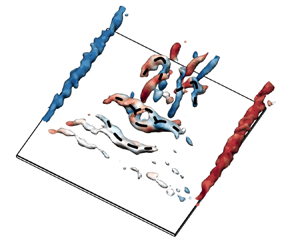
Figure 10 presents an overview of the instantaneous vortical structures for the representative  ${A{\kern-4pt}R} = 1.00$ case. In this study, vortical structures are depicted through the
  $Q$-criterion (Hunt, Wray & Moin Reference Hunt, Wray and Moin1988; Jeong & Hussain Reference Jeong and Hussain1995), where
  $Q$ is defined by the second invariant of the velocity gradient tensor. The iso-surfaces of
  $Qc^2/U_\infty ^2 = 30$ are shown and coloured according to the streamwise vorticity. The effect of the
  $Q$ threshold (
 $Q_{th}=30$) on the characterization of vortex evolution is demonstrated in the Appendix. Near the midspan, the separated shear layer rolls up and forms C-shape vortices. As these C-shape vortices move downstream, they undergo complex transformations, such as the splitting of vortex heads. As shown in figure 10, the split vortex resembles the Old English letter ‘Þ’ (thorn), thus is named the Þ-shape vortex. Further downstream, several hairpin vortices begin to take shape simultaneously. The visualization of instantaneous LEVs highlights two essential processes: (i) the transformation of C-shape vortices, and (ii) the formation of hairpin vortices. These processes are inspected in more detail below. Supplementary movie 1 in the supplementary material, available at https://doi.org/10.1017/jfm.2024.169, shows the evolution of vortical structures for the representative
  ${A{\kern-4pt}R} = 1.00$ case.

Figure 10. Instantaneous flow field for  ${A{\kern-4pt}R} = 1.00$. The vortical structures are visualized using the iso-surfaces of
  $Qc^2/U_\infty ^2 = 30$, which are coloured according to the streamwise vorticity.
5.1. The LEV transformation process
To understand the transformation mechanisms of C-shape vortices, the interactions between the near-wall spanwise flow and the LEVs are investigated in this subsection. A phase-averaging technique is employed to unveil the underlying flow physics. Specifically, § 5.1.1 focuses on the interaction mechanisms, while § 5.1.2 discusses the subsequent vortex transformations.
Before introducing the phase-averaging technique, the near-wall spanwise flow is characterized. Figure 11(a) presents the distribution of the instantaneous near-wall spanwise flow for the  ${A{\kern-4pt}R} = 1.00$ case in a plane parallel to the plate, situated
  $0.02c$ vertically from the top surface of the plate. The spanwise flow regions are demarcated by the magenta solid lines of
  $| w |/{U_\infty } = 0.05$. To evaluate the unsteady characteristics of the near-wall spanwise flow, the spanwise interval of the spanwise flow regions near the midspan is denoted by
  $d_w(x, t)$. This is exemplified in figure 11(a) by the black double-arrowed line. Moreover, the power spectral density of
  $d_w$ is presented in figure 11(b). The power spectral density is calculated by employing the same method as in figure 9. The presence of distinct peaks at
  $St_1$ for
  ${A{\kern-4pt}R} \leq 1.38$ is evident, while no peak is detected within the vortex-shedding frequency range (masked in red) for
  ${A{\kern-4pt}R} = 1.50$. These spectral characteristics suggest the existence of interactions between the near-wall spanwise flow and the shed LEVs for the
  ${A{\kern-4pt}R} \leq 1.38$ cases.

Figure 11. (a) Instantaneous spanwise velocity distribution in the plane at vertical distance  $0.02c$ from the top surface of the plate for
  ${A{\kern-4pt}R} = 1.00$. The magenta solid lines are the contour lines of
  $| w |/{U_\infty } = 0.05$. (b) Power spectral density map of the spanwise interval of the near-wall spanwise flow region,
  $d_w$. The region masked in red corresponds to the vortex-shedding frequency range.
To elucidate the dynamic evolution of the near-wall spanwise flow and its interactions with the LEVs, we employ the phase-averaging technique. First, the phase information is identified using the POD method. Note that the fluctuating velocity fields are decomposed within a volume size  $[0.2c, 0.8c]\times [0, 0.22c] \times [-0.3c {A{\kern-4pt}R}, 0.3c {A{\kern-4pt}R} ]$. The downstream boundary
  $x/c = 0.8$ lies approximately upstream of the position where the horseshoe vortices appear, ruling out the horseshoe vortex formation process. Additionally, the spanwise and vertical extents of the subdomain are chosen to facilitate comparison of LEVs at different
  ${A{\kern-4pt}R}$ values and to minimize the effect of measurement noise. In particular, the spanwise range is
  ${A{\kern-4pt}R}$-dependent in order to exclude the tip region. After identifying the phases, an eight-term Fourier model is employed to fit the phase-sorted instantaneous velocity vectors at each spatial point. For more details on our implementation, refer to Zhu et al. (Reference Zhu, Wang, Xu, Qu and Long2023b).
The feasibility of phase identification, which is crucial for accurate phase averaging results, is evaluated in figure 12. Figure 12(a) presents the  ${TKE}$ contribution of the first
  $15$ POD modes, and figure 12(b) presents the power spectral density of the first mode pair used for phase identification. The power spectral density is calculated by employing the same method as used in figure 9. Figure 12(a) illustrates that the first two POD modes share similar energy levels for each
  ${A{\kern-4pt}R}$ case, exceeding those of the remaining modes by at least a factor of 2. Furthermore, the time coefficients of the first mode pair have identical spectral content, as illustrated in figure 12(b). Note that the spectral peaks at
  $St_1$ are easily distinguishable for this conjugated mode pair. Hence, it is reasonable to associate the first two dominant POD modes with the convection of LEVs. In other words, the phase information of the LEV convection can be identified accurately through the POD analysis.

Figure 12. The POD results for the fluctuating velocity fields. (a) The  ${TKE}$ contribution of the first
  $15$ POD modes. (b) Power spectral density of the first mode pair used for phase identification. The region masked in red corresponds to the vortex-shedding frequency range.
Figure 13 presents the distribution of the phase-averaged spanwise interval of the near-wall spanwise flow region,  $\widehat {d_w} (x, \theta )$. It is observed that
  $\widehat {d_w}$ oscillates with
  $\theta$ downstream of
  $x/c \approx 0.4$ for
  ${A{\kern-4pt}R} \leq 1.38$. This oscillatory behaviour is characterized by the phase angle
  $\theta _w$, where
  $\widehat {d_w}$ reaches its minimum value at each given streamwise position. It should be noted that a decrease in
  $\widehat {d_w}$ implies a greater influence of spanwise fluid transport on the flow near the midspan. The resulting mappings of
  $\theta _w$–
 $x$ are essentially the valley lines of the
  $\widehat {d_w}$ distribution, marked with red solid lines in figure 13.

Figure 13. Distribution of the phase-averaged spanwise interval of the near-wall spanwise flow region,  $\widehat {d_w} (x, \theta )$. The red dots indicate the condition where the LEV is located at
  $\hat {x}_c = 0.45$. The magenta dots correspond to
  $\hat {x}_c = 0.54$ for
  ${A{\kern-4pt}R} = 1.00$, and
  $\hat {x}_c = 0.56$ for
  ${A{\kern-4pt}R} \geq 1.25$.
To provide comprehensive insights into the interactions between the near-wall spanwise flow and the LEVs, we track the evolution of the LEVs via their streamwise positions  $\hat {x}_c$. These streamwise positions are determined by the equation
  $\hat {x}_c = {\iint _{C}{x{{{\hat {\omega }}}_{z}}\,\textrm {d}S}}/{\iint _{C}{c{{{\hat {\omega }}}_{z}}\,\textrm {d}S}}$, where
  $C$ is the integral region defined as the
  $\hat {Q}c^2/U_\infty ^2 \geq 30$ region in the midspan plane. The resulting mappings
  $\theta$–
 $\hat {x}_c$ are marked as black dots in figure 13. As
  ${A{\kern-4pt}R}$ decreases, the mappings
  $\theta$–
 $\hat {x}_c$ become detectable further upstream, particularly for
  ${A{\kern-4pt}R} = 1.00$. This implies that the C-shape vortex sheds further upstream, and supports that the disturbances associated with vortex shedding in the shear layer are amplified by the spanwise fluid transport.
Examination of the mappings  $\theta _w$–
 $x$ and
  $\theta$–
 $\hat {x}_c$ reveals two significant regions, labelled as
  $A$ and
  $B$ in figure 13. For
  ${A{\kern-4pt}R} \leq 1.38$, region
  $A$ appears where the streamwise distance between the two mappings is essentially constant. That is, as the C-shape vortex moves downstream, the flow on the windward side of its head is affected persistently by the near-wall spanwise flow. This agrees with the presence of the peaks at
  $St_1$ in the
  $d_w$ spectra for the
  ${A{\kern-4pt}R} \leq 1.38$ cases (see figure 11b). Moreover, region
  $B$ is characterized by the splitting of the LEVs in the midspan plane, which appears for the
  ${A{\kern-4pt}R} \leq 1.25$ cases. Additional insights are provided by comparing the phase-averaged flow fields for different
  ${A{\kern-4pt}R}$ values, which are presented below.
5.1.1. Interaction mechanism
Figure 14 presents plan views of the phase-averaged flow fields corresponding to  $\hat {x}_c = 0.45$ (indicated by the red dots in figure 13). The grey iso-surfaces of
  $\hat {Q}c^2/U_\infty ^2 = 30$ represent the LEVs, while the transparent yellow iso-surfaces of
  $\hat {v}/U_\infty = 0.075$ depict the upwash flow. The streamwise positions where
  $\widehat {d_w}$ reaches its minimum value at the corresponding phase are shown by the magenta lines. As
  ${A{\kern-4pt}R}$ decreases, a noticeable enhancement in the upwash flow is observed between the magenta line and the windward side of the C-shape vortex head. This demonstrates that the near-wall spanwise flow pumps fluid to the windward side of the vortex head, thereby enhancing the localized upwash. The enhanced upwash results in a larger shear strength and feeds additional vorticity, thereby strengthening the vortex head. These results are consistent with the conjecture in Zhu et al. (Reference Zhu, Wang, Xu, Qu and Long2023b).

Figure 14. Plan views of the phase-averaged flow fields corresponding to  $\hat {x}_c = 0.45$. The magenta lines correspond to the streamwise positions where
  $\widehat {d_w}$ reaches its minimum value at the corresponding phase. The LEVs are represented using the grey iso-surfaces of
  $\hat {Q}c^2/U_\infty ^2 = 30$. The transparent yellow and blue iso-surfaces correspond to
  $\hat {v}/U_\infty = 0.075$ and
  $\widehat {u^\prime v^\prime }/U_\infty ^2= -0.006$, respectively.
The strengthening of the vortex head is examined further by comparing the magnitude of entrainment. The phase-averaged Reynolds stress  $\widehat {u^\prime v^\prime }/U_\infty ^2$ is used as a measure of entrainment. As shown in figure 14, the transparent blue iso-surfaces correspond to
  $\widehat {u^\prime v^\prime }/U_\infty ^2= -0.006$. As
  ${A{\kern-4pt}R}$ decreases, a noticeable increase in
  $\widehat {u^\prime v^\prime }/U_\infty ^2$ is detected on the leeward side of the C-shape vortex. This indicates that the interactions contribute to the flow mixing, entraining high-momentum fluid from the outer flow towards the plate surface. Overall, the interaction between the near-wall spanwise flow and the LEV results in a localized upwash flow on the windward side of the vortex head. The upwash flow feeds vorticity to the LEV head, thus strengthening the vortex head and the associated entrainment.
5.1.2. Transformation of C-shape vortices
Having explained the mechanism underlying the interactions between the near-wall spanwise flow and the LEVs, next we investigate the transformation of the C-shape vortices downstream.
Figure 15 presents plan views of the flow fields corresponding to  $\hat {x}_c = 0.54$ for
  ${A{\kern-4pt}R} = 1.00$, and
  $\hat {x}_c = 0.56$ for
  ${A{\kern-4pt}R} \geq 1.25$ (indicated by the magenta dots in figure 13). The LEVs are shown by the grey iso-surfaces of
  $\hat {Q}c^2/U_\infty ^2 = 30$. For the
  ${A{\kern-4pt}R} = 1.00$ and
  $1.25$ cases, as the C-shape vortex develops downstream, it splits near the midspan, resulting in the formation of the Þ-shape vortex. This phenomenon is referred to as the coherent vortex-splitting behaviour, which can be observed in the instantaneous flow field (see figure 10). By contrast, for the
  ${A{\kern-4pt}R} = 1.38$ and
  $1.50$ cases, the C-shape vortex morphs into the M-shape vortex. This LEV behaviour is consistent with the observations in previous work (Zhu et al. Reference Zhu, Wang, Xu, Qu and Long2023b) on the trapezoidal plate with
  ${A{\kern-4pt}R} = 1.38$.

Figure 15. Plan views of the phase-averaged flow fields corresponding to  $\hat {x}_c = 0.54$ for
  ${A{\kern-4pt}R} = 1.00$, and
  $\hat {x}_c = 0.56$ for
  ${A{\kern-4pt}R} \geq 1.25$. The iso-surfaces of
  $\hat {Q}c^2/U_\infty ^2 = 30$ are shown in grey representing the LEVs.
As a supplement to figure 15, we conduct a statistical analysis of the instantaneous streamwise positions  $x_c$ and the corresponding spanwise circulations
  $\varGamma _{cz}$ of the LEVs. These LEV parameters are determined by equations
  $x_c={\iint _{C}{x{\omega _z}\,\textrm {d}S}}/{\iint _{C}{c{\omega _z}\,\textrm {d}S}}$ and
  $\varGamma _{cz} ={\iint _{C}{{\omega _z}\,\textrm {d}S}}/{(U_\infty c)}$. The integral region
  $C$ is defined as the
  $Qc^2/U_\infty ^2 \geq 30$ region in the midspan plane, consistent with that in figure 13. The obtained probability distributions are presented in figure 16. The red lines display the primary development routine for the LEVs. The magenta triangles denote the locations where the C-shape vortices split in the phase-averaged flow fields for the
  ${A{\kern-4pt}R} = 1.00$ and
  $1.25$ cases. Notably, there are regions of high probability for
  $\varGamma _{cz}$ near these triangles, as indicated by the magenta dashed boxes. The occurrence of these regions can be attributed to the splitting behaviour of LEVs. However, this feature cannot be identified for the
  ${A{\kern-4pt}R} = 1.38$ and
  $1.50$ cases. These findings confirm the occurrence and the dominance of the coherent vortex-splitting behaviour for the
  ${A{\kern-4pt}R} = 1.00$ and
  $1.25$ cases.

Figure 16. Probability distribution of the instantaneous spanwise circulation  $\varGamma _{cz}$ of the LEVs. The red lines display the primary development path of the LEVs. The magenta triangles denote the locations where the C-shape vortices split in the phase-averaged flow fields for
  ${A{\kern-4pt}R} = 1.00$ and
  $1.25$. The magenta dashed boxes indicated regions of high probability for
  $\varGamma _{cz}$ near the magenta triangles.
An intriguing fact arises that the  $\varGamma _{cz}$ distribution becomes more concentrated around the red line as
  ${A{\kern-4pt}R}$ decreases, while the spatial growth rate of
  $\varGamma _{cz}$ changes little. This indicates a more regular development of LEVs due to stronger tip effects, as explained below. For
  ${A{\kern-4pt}R} \geq 1.38$, several instabilities are active in the amplification of disturbances, affecting the subsequent breakup of LEVs. Consequently, it becomes statistically impossible to distinguish the vortex breakup behaviours. As
  ${A{\kern-4pt}R}$ decreases to
  $1.25$ and
  $1.00$, the aforementioned LEV/spanwise-flow interactions sustain the coherence of the LEVs until the vortex heads split. Meanwhile, the stronger downwash restricts the disturbance growth, which makes the identified vortex-splitting behaviour more prominent. With the co-action of the spanwise fluid transport and the downwash, the coherent vortex-splitting behaviour dominates the LEV evolution and manifests in the probability distribution.
5.2. The hairpin vortex formation process
It is well known that hairpin vortices are important structures in the wake of low- ${A{\kern-4pt}R}$ plates and play significant roles in wake instability and force generation (Taira & Colonius Reference Taira and Colonius2009; Menon, Kumar & Mittal Reference Menon, Kumar and Mittal2022). It is therefore valuable to thoroughly understand the formation process of hairpin vortices.
Two fundamental processes in the formation of hairpin vortices are illustrated in figure 17 for the  ${A{\kern-4pt}R} = 1.00$ case. These processes are distinguished by whether the LEVs merge near the midspan. Figure 17(a) shows the process without vortex merging. At
  $tU_\infty /c = 4.61$, the LEV has split into two parts at its head, becoming the Þ-shape vortex. The two parts of the split vortex head, upstream and downstream, are denoted by V1-u and V1-d, respectively. The unsplit vortex arms are denoted by V1-a. During the downstream convection, V1-d gradually dissipates, while V1-u moves downstream at a slower rate than V1-a. This causes V1-a to stretch and tilt, thus evolving into two adjacent hairpin vortices.

Figure 17. Time series showing two fundamental processes for hairpin vortex formation ( ${A{\kern-4pt}R} = 1.00$): (a) without vortex merging, and (b) with vortex merging. Vortical structures are visualized using the iso-surfaces of
  $Qc^2/U_\infty ^2 = 30$, which are coloured according to the streamwise vorticity.
Figure 17(b) presents the alternative typical process in which the LEVs merge near the midspan. In addition to the Þ-shape vortex, the subsequent C-shape vortex is involved in this process and denoted by V2. Similarly, the three parts of the Þ-shape vortex are denoted by V1-u, V1-d and V1-a, respectively. During the downstream convection, V1-d dissipates, while V1-u merges with V2 instead of moving downstream. After vortex merging, the lateral arms of the subsequent C-shape vortex (denoted by V2-a) develop into two hairpin vortices positioned side by side. Simultaneously, the merged vortex head (V2-m) evolves into another hairpin vortex at a higher position.
To account for the influence of  ${A{\kern-4pt}R}$, figure 18 depicts a representative process for the
  ${A{\kern-4pt}R} = 1.50$ case. During this process, due to the weakening of the tip effects, the LEV splits at the two spanwise portions concurrently. Figure 18(a) presents two LEVs denoted by V1 and V2. As V2 moves downstream, it transforms into the M-shape structure. Meanwhile, the downstream V1 splits at its shoulders, emphasized by the magenta dashed circles in figure 18(b). The upstream and downstream parts of the split V1 are denoted by V1-u and V1-d, respectively. Similar to the vortex merging behaviour observed in figure 17(b), the two V1-u merge with V2, while the two V1-d dissipate. Finally, the two merged portions evolve into two hairpin vortices at the top, and the remaining portions into another three hairpin vortices at the bottom.

Figure 18. Time series showing a representative hairpin vortex formation process for  ${A{\kern-4pt}R} = 1.50$. Vortices are visualized using the iso-surfaces of
  $Qc^2/U_\infty ^2 = 30$, which are coloured according to the streamwise vorticity.
Based on the observations, the formation of hairpin vortices is dominated by two identified fundamental processes once the vortex splitting occurs. For the  ${A{\kern-4pt}R} = 1.00$ and
  $1.25$ cases, the formation of hairpin vortices alternates solely between these two fundamental processes after the coherent vortex-splitting behaviour. Although the splitting of LEVs occurs irregularly in a spanwise range near the midspan for the
  ${A{\kern-4pt}R} = 1.38$ and
  $1.50$ cases, the identified fundamental process can still be identified. Thus the two identified formation processes enable a fundamental understanding of the formation of hairpin vortices for larger
  ${A{\kern-4pt}R}$ values.
6. Summary and conclusions
The present study investigates the three-dimensional flows over four low- ${A{\kern-4pt}R}$ rectangular plates at angle of attack
  $\alpha = 6^\circ$ and chord Reynolds number
  ${\textit {Re}}_c=5400$ using both tomographic and planar PIV techniques. The
  ${A{\kern-4pt}R}$ values tested include 1.00, 1.25, 1.38 and 1.50. The decrease in
  ${A{\kern-4pt}R}$ leads to a greater influence of spanwise fluid transport on the flow, providing fresh and valuable insights into the underlying mechanisms. The novelty of this study lies in revealing the interplay between the spanwise fluid transport and the downwash.
The fundamental evolution routine of the vortical structures can be divided into four stages qualitatively: (i) the development of separated shear layer; (ii) the convection of C-shape vortices, where the near-wall spanwise flow interacts with the C-shape vortices; (iii) the transformation of C-shape vortices; and (iv) the formation of hairpin vortices. This LEV evolution routine is summarized schematically in figure 19, along with the underlying mechanisms associated with the spanwise fluid transport.

Figure 19. Conceptional sketch for the fundamental evolution routine of the vortical structures for low- ${A{\kern-4pt}R}$ plates. The orange and magenta arrows indicate two mechanisms associated with the spanwise fluid transport, which are revealed in this study.
The development of the separated shear layer is modulated by both spanwise fluid transport and downwash. Spanwise fluid transport amplifies the disturbances associated with vortex shedding by enhancing the reverse-flow intensity. Thus it promotes the shear layer roll-up and subsequent vortex shedding. Conversely, downwash suppresses the growth of all disturbances.
The role of spanwise fluid transport on the subsequent LEV development is clarified. The interactions between the near-wall spanwise flow and the LEVs occur for  ${A{\kern-4pt}R} \leq 1.38$. As the LEV convects downstream, the near-wall spanwise flow pumps persistently fluid towards the windward side of the C-shape vortex head, and promotes a localized upwash flow on the windward side. This localized upwash strengthens the vortex head by feeding additional vorticity. As a result, the interaction can sustain the coherent development of C-shape vortices.
A novel vortex-splitting transformation is found for  ${A{\kern-4pt}R} \leq 1.25$. Specifically, as the C-shape vortex develops downstream, it splits into two parts at its head in a regular fashion, and becomes the Þ-shape vortex. This novel transformation supplements the already discovered transformation from a C-shape vortex into an M-shape vortex (for
  ${A{\kern-4pt}R} \geq 1.38$ in this study, and see Zhu et al. Reference Zhu, Wang, Xu, Qu and Long2023b). Furthermore, the underlying mechanism is revealed. Mainly, the spanwise fluid transport is sufficient to sustain the coherence of the LEVs until the splitting of the vortex heads occurs. In addition, the stabilizing effect of the downwash also contributes to the dominance of the coherent vortex-splitting behaviour. Following the vortex-splitting transformation, two fundamental processes for the formation of hairpin vortices are identified for the first time. The two processes occur alternately. Depending on whether the vortex heads merge near the midspan, two or three hairpin vortices are formed simultaneously. The vortex behaviours described above can still be identified for the larger
  ${A{\kern-4pt}R}$ values tested. Therefore, the evolution routine obtained in this study provides a fundamental understanding of the complex vortex evolution for low-
 ${A{\kern-4pt}R}$ plates.
In general, this study deepens the understanding of the tip effects on the formation of three-dimensional flows over low- ${A{\kern-4pt}R}$ plates. The downwash stabilizes the flow, while the spanwise fluid transport promotes the LEV shedding and sustains the subsequent coherent development of the LEVs. There are important analogies between the spanwise flow patterns on the steadily translating plate and the dynamic manoeuvring plates (Yilmaz & Rockwell Reference Yilmaz and Rockwell2010, Reference Yilmaz and Rockwell2012). In particular, the spatial distribution of LEVs and near-wall spanwise flows in these studies suggests that the interactions between them are likely also present. Therefore, the flow physics revealed in the present study may be useful for a better understanding of flows over manoeuvring plates. Moreover, the associated flow physics can provide guidance for flow control strategies that could potentially improve the cruising and gliding performance of MAVs. The feasibility has been discussed in our previous study (Zhu et al. Reference Zhu, Wang, Xu, Qu and Long2023b). Thus the revealed flow physics can play a role in the design of state-of-the-art MAVs. Finally, the interactions between the near-wall spanwise flow and the vortical structures may also shed light on other three-dimensional flows, such as the wake of a notchback Ahmed body (He et al. Reference He, Minelli, Wang, Dong, Gao and Krajnović2021) and ship airwakes (Zhu et al. Reference Zhu, Zhang, Gnanamanickam and Gordon Leishman2023a).
Supplementary movie
A supplementary movie is available at https://doi.org/10.1017/jfm.2024.169.
Acknowledgements
We thank the anonymous referees for their constructive comments in improving this paper.
Funding
This work was supported by the National Natural Science Foundation of China (no. 11721202).
Declaration of interests
The authors report no conflict of interest.
Appendix. Effect of  $Q$ threshold on characterization of vortex evolution

In this study, we have selected  $Q_{th} = 30$ as a representative threshold and characterized the vortex evolution with different
  ${A{\kern-4pt}R}$ values. Here, three other
  $Q_{th}$ values (
 $Q_{th} = 25, 35, 40$) are examined to elucidate the sensitivity of our findings to the
  $Q_{th}$ value. The conclusion is that the flow physics revealed is not affected by the choice of the
  $Q_{th}$ value.
The focus is first placed on the phase-averaged flow fields, as shown in figure 20. The distributions of  $\widehat {d_w}$ and
  $\theta _w-x$ (i.e. the red solid lines) are also presented for better comparison. Distinct variations in vortex evolution with
  $Q_{th}$ appear for the
  ${A{\kern-4pt}R} = 1.00$ and
  $1.25$ cases. Note that in this
  ${A{\kern-4pt}R}$ range, the vortex-splitting behaviour occurs. When the
  $Q_{th}$ value is too large (e.g.
  $Q_{th} = 40$, as highlighted by the green region in figure 20), the downstream part of the split vortex cannot be identified. It suggests that the upstream part of the split vortex is stronger than the downstream part. This is consistent with the observations in the hairpin vortex formation process, where the downstream part of the split vortex disappears. As for the too small
  $Q_{th}$ value (e.g.
  $Q_{th} = 25$, as highlighted by the blue region in figure 20), the entire split vortex region is extracted, so that no bifurcation pattern can be distinguished from the distribution of black dots. Therefore, different features of the vortex-splitting behaviour are brought out by varying the
  $Q$ threshold. As is evident from figure 20(b), the appropriate
  $Q$ threshold should be in the range
  $30 \lesssim Q_{th} \lesssim 35$ to illustrate the vortex-splitting behaviour thoroughly.

Figure 20. Distribution of the streamwise positions  $\hat {x}_c$ of LEVs corresponding to
  $Q_{th} = 25$, 35 and
  $40$.
$40$.
Moreover, the flow physics revealed in the present study is independent of the selected  $Q$ threshold. Despite the
  $Q_{th}$ variation, the vortex-splitting behaviour can be identified only for the
  ${A{\kern-4pt}R} = 1.00$ and
  $1.25$ cases, while only negligible changes in the black dot distribution are seen for the
  ${A{\kern-4pt}R} = 1.38$ and
  $1.50$ cases. This means that the Þ-shape vortices cannot be identified for the higher
  ${A{\kern-4pt}R}$ cases, even if applying a higher
  $Q$ threshold.
An additional consideration is the probability distribution of the instantaneous spanwise circulation,  $\varGamma _{cz}$. Here, the circulation
  $\varGamma _{cz}$ is calculated with
  $Q_{th} = 25, 35, 40$. The results are shown in figure 21. Despite the
  $Q_{th}$ variation, the high probability distribution of
  $\varGamma _{cz}$ is still observable close to where the vortices split, as indicated by the magenta dashed boxes for the
  ${A{\kern-4pt}R} = 1.00$ and
  $1.25$ cases. Note that for the
  ${A{\kern-4pt}R} = 1.00$ case, the phase-averaging analysis indicates that the entire split vortex region should be extracted by
  $Q_{th} = 25$. Thus the appearance of the high probability distribution in the magenta boxes may be attributed to the sudden circulation reduction of the entire split vortex region during the vortex-splitting process. However, this high probability distribution cannot be identified for the
  ${A{\kern-4pt}R} = 1.38$ and
  $1.50$ cases. These results confirm that the high probability distribution in the magenta boxes is the footprint of the coherent vortex-splitting behaviour, which occurs only for the
  ${A{\kern-4pt}R} = 1.00$ and
  $1.25$ cases.

Figure 21. Probability distributions of the instantaneous spanwise circulation  $\varGamma _{cz}$ of the LEVs. Here, the circulation
  $\varGamma _{cz}$ is calculated with
  $Q_{th} = 25, 35, 40$. The magenta triangles denote the locations where the C-shape vortices split in the phase-averaged flow fields for
  ${A{\kern-4pt}R} = 1.00$ and
  $1.25$. The magenta dashed boxes indicated regions of high probability for
  $\varGamma _{cz}$ near the magenta triangles.
In all, the flow physics revealed is independent of the chosen  $Q$ threshold. The novel vortex-splitting transformation occurs only for the
  ${A{\kern-4pt}R} = 1.00$ and
  $1.25$ cases. The underlying mechanism is attributed to the spanwise fluid transport, but rather the selection of the
  $Q$ threshold.


