


1. Introduction
One of the most noticeable properties of the wall-bounded turbulent flows is the enhancement of transport processes, e.g. transports of mass, momentum and heat, and thus understanding the near-wall turbulence is important because the prediction and control of the near-wall turbulence are beneficial from the engineering point of view (Jiménez Reference Jiménez2012). It is well known that the near-wall flow fields in the turbulent boundary layers are organized into streaky coherent structures which consist of high- and low-speed fluids that are elongated in the streamwise direction and alternating in the spanwise direction, and the manipulation of the near-wall coherent structures is an effective way to control the flows (Choi, Moin & Kim Reference Choi, Moin and Kim1994). Historically, the attempts to understand the characteristics of the wall turbulence from the perspective of coherent motions date back at least to the work of Theodorsen (Reference Theodorsen1952). Then, the near-wall coherent structures in the turbulent boundary layer were observed by Hama, Long & Hegarty (Reference Hama, Long and Hegarty1957) and Kline et al. (Reference Kline, Reynolds, Schraub and Runstadler1967), which showed the existence of sublayer streaks visually. The visualizations of the ejection motion, which is the upward motion of the low-speed fluid (Corino & Brodkey Reference Corino and Brodkey1969), and large coherent structures in free-shear layers (Brown & Roshko Reference Brown and Roshko1974) followed. Furthermore, it was revealed that the near-wall coherent structures play an important role in the production of Reynolds stress (Kim, Kline & Reynolds Reference Kim, Kline and Reynolds1971) and quasi-streamwise vortices (Blackwelder & Eckelmann Reference Blackwelder and Eckelmann1979), and thus the coherent structures are the key players for the near-wall autonomous turbulence regeneration cycle (Jiménez & Moin Reference Jiménez and Moin1991; Hamilton, Kim & Waleffe Reference Hamilton, Kim and Waleffe1995; Jiménez & Pinelli Reference Jiménez and Pinelli1999). Through these pioneering works, the study of wall-bounded turbulent flows started to pay more attention to the near-wall coherent structures, and reviews on the coherent structures have also been presented by Robinson (Reference Robinson1991), Panton (Reference Panton2001), Adrian (Reference Adrian2007) and Jiménez (Reference Jiménez2018). The studies on near-wall coherent structures have also revealed the turbulence structures in the outer layer, e.g. hairpin-like vortices (Head & Bandyopadhyay Reference Head and Bandyopadhyay1981; Kim, Moin & Moser Reference Kim, Moin and Moser1987), and the turbulent motions in the near-wall region interact with the large-scale outer motions; one of the most intense interactions is the sudden eruptions of the near-wall fluid into the outer region, which is named bursting by Kim et al. (Reference Kim, Kline and Reynolds1971). Furthermore, active modulation effects of the near-wall motions by the outer-layer large-scale structures have also been recognized in relatively recent studies (Hutchins & Marusic Reference Hutchins and Marusic2007; Mathis, Hutchins & Marusic Reference Mathis, Hutchins and Marusic2009; Chung & McKeon Reference Chung and McKeon2010; Bernardini & Pirozzoli Reference Bernardini and Pirozzoli2011; Mathis, Hutchins & Marusic Reference Mathis, Hutchins and Marusic2011; Hwang Reference Hwang2013). In the early days, when the studies on the turbulence coherent structures were mainly relying on limited probe measurements, several conditional sampling techniques were developed to identify the statistical properties of the turbulence structures, especially for elucidating a series of the bursting process; lift-up, oscillation, break-up and ejection of the low-speed streaks. For example, variable-interval time average by Blackwelder & Kaplan (Reference Blackwelder and Kaplan1976), variable-interval space average by Kim (Reference Kim1985) and quadrant analysis by Wallace, Eckelmann & Brodkey (Reference Wallace, Eckelmann and Brodkey1972), Willmarth & Lu (Reference Willmarth and Lu1972) and Lu & Willmarth (Reference Lu and Willmarth1973). Bogard & Tiederman (Reference Bogard and Tiederman1986) surveyed these techniques comprehensively and concluded that the quadrant analysis is the best compromise in terms of the detection probability and false positives.
Thanks to the recent rapid progress of high-performance computers, the large-eddy simulation (LES) technique has been gaining more attention as a turbulent flow simulation tool and replacing the traditional Reynolds-averaged Navier–Stokes (RANS) simulations in both academic and engineering fields. The higher potential of the LES to predict the unsteady turbulent flows more accurately is attributed to the direct resolution of energy-carrying dominant eddies on the computational grid, whereas all unsteady eddy dynamics is modelled in RANS. This modelling strategy makes the LES more attractive in terms of the compromise between the computational cost and accuracy, compared with direct numerical simulation (DNS) and RANS. However, the advantage of the LES described above is not the case for wall-bounded turbulent flows including a solid boundary. The wall-bounded turbulent flows are multi-scale phenomena, and the quasi-streamwise vortices dominating the flow dynamics near the solid wall scaled with the viscous length scale represented by  $\delta _\nu =\nu _w/u_\tau$ instead of the local boundary-layer thickness
  $\delta$, where
  $\nu _w$ is the kinematic viscosity at the wall, and
  $u_\tau$ is the friction velocity defined as
  $u_\tau =\sqrt {\tau _w/\rho _w}$ using the shear stress
  $\tau _w$ and the density
  $\rho _w$ at the wall. This indicates that the ratio of the length scales between the near-wall eddies scaled with the viscous length
  $\delta _\nu$ and outer-layer eddies scaled with the boundary-layer thickness
  $\delta$ increases, at increasing Reynolds number
  $Re_\tau =\delta /\delta _\nu$ (Smits, McKeon & Marusic Reference Smits, McKeon and Marusic2011). This causes the near-wall resolution problem of the LES for the wall-bounded turbulent flow simulations and makes the computational cost highly prohibitive even if a state-of-the-art supercomputer is employed, especially at high Reynolds numbers. Therefore, some methodologies are required to make LES applicable to high Reynolds number wall-bounded turbulent flow simulations that emerge in actual engineering problems, e.g. the Reynolds number of a commercial airplane is
  $Re_c \sim 10^7$ based on the mean aerodynamic chord of the wing.
The near-wall modelling for LES, which models the inner-layer turbulence rather than the direct resolution, has been studied over the past several decades to overcome the near-wall resolution problem since Deardorff (Reference Deardorff1970), as an alternative tool of the wall-resolved LES (WRLES) resolving the energy-carrying eddies down to the wall. Several methodologies have been proposed in the framework of near-wall modelling (Piomelli & Balaras Reference Piomelli and Balaras2002; Piomelli Reference Piomelli2008; Larsson et al. Reference Larsson, Kawai, Bodart and Bermejo-Moreno2016; Bose & Park Reference Bose and Park2018), and the approaches are classified into the following two categories; (i) LES/RANS hybrid model and (ii) wall-stress model as discussed by Larsson et al. (Reference Larsson, Kawai, Bodart and Bermejo-Moreno2016). The first category is the methodology that blends the near-wall RANS and sub-grid-scale (SGS) eddy viscosities for the outer-layer LES, and the detached eddy simulation first proposed by Spalart (Reference Spalart1997) (the progress afterward was reviewed in Spalart Reference Spalart2009) is one of the most representative methods. The switching location of the eddy viscosities between RANS and SGS is usually specified either explicitly or implicitly. The second category is the methodology that models the wall-shear stress  $\tau _w$ directly, and the calculation of the LES is conducted down to the wall, which means no blending of RANS and SGS eddy viscosities is required (Larsson et al. Reference Larsson, Kawai, Bodart and Bermejo-Moreno2016; Bose & Park Reference Bose and Park2018). The focus of the present study is the latter wall-stress model, and throughout this paper, the term ‘wall-modelled LES (WMLES)’ is used to refer to the wall-stress model. The pioneering work by Chapman (Reference Chapman1979) estimated the number of computational grid points required for the DNS, WRLES and WMLES, respectively, which has been revisited by Choi & Moin (Reference Choi and Moin2012), and most recently by Yang & Griffin (Reference Yang and Griffin2021). According to Choi & Moin (Reference Choi and Moin2012), the total number of grid points
  $N$ required for the DNS, WRLES and WMLES are estimated to be
  $N_{DNS}\sim Re^{37/14}$,
  $N_{WRLES}\sim Re^{13/7}$ and
  $N_{WMLES}\sim Re$, respectively. It is obvious that the computational cost of the WRLES is still prohibitively high, however, the WMLES is more favourable than the WRLES.
The focus of the present study is to reveal the fundamental near-wall flow physics of the WMLES, not having been investigated in the past study, and to contribute to the further understanding and developments of the WMLES, since the prior studies on the WMLES have mainly focused on either model developments (e.g. Kawai & Larsson Reference Kawai and Larsson2012, Reference Kawai and Larsson2013; Bose & Moin Reference Bose and Moin2014; Park & Moin Reference Park and Moin2014; Yang et al. Reference Yang, Sadique, Mittal and Meneveau2015; Yang, Park & Moin Reference Yang, Park and Moin2017; Bae et al. Reference Bae, Lozano-Durán, Bose and Moin2019; Yang et al. Reference Yang, Zafar, Wang and Xiao2019; Tamaki & Kawai Reference Tamaki and Kawai2021; Kamogawa, Tamaki & Kawai Reference Kamogawa, Tamaki and Kawai2023), or applications (e.g. Bermejo-Moreno et al. Reference Bermejo-Moreno, Campo, Larsson, Bodart, Helmer and Eaton2014; Park Reference Park2017; Fukushima & Kawai Reference Fukushima and Kawai2018; Yang et al. Reference Yang, Urzay, Bose and Moin2018; Tamaki et al. Reference Tamaki, Fukushima, Kuya and Kawai2020; Lozano-Durán, Bose & Moin Reference Lozano-Durán, Bose and Moin2022; Mettu & Subbareddy Reference Mettu and Subbareddy2022; Asada et al. Reference Asada, Tamaki, Takaki, Yumitori, Tamura, Hatanaka, Imai, Maeyama and Kawai2023). As described above, the fundamental concept of the WMLES is to avoid resolving the near-wall Reynolds-number-dependent small eddies, whereas the large energy-dominant eddies in the outer layer are directly resolved on the computational grid and the LES calculation is conducted down to the wall. By appropriately estimating the wall-shear stress used as a flux boundary condition, the WMLES reproduces the outer-layer turbulence statistics in the attached turbulent boundary layer, such as the mean streamwise velocity and Reynolds shear stress. The success of the WMLES in the accurate predictions of the turbulence statistics is explained by the streamwise momentum conservation law in the inner turbulent boundary layer (Kawai & Larsson Reference Kawai and Larsson2012)
 \begin{equation} \overline{{\mu}_{t,sgs}} \partial_y \tilde{u}-\bar{\rho}\widetilde{u''v''}\approx\overline{\tau_w}, \end{equation}
where  $\overline {\mu _{t,sgs}}$ is the SGS eddy viscosity,
  $-\bar {\rho }\widetilde {u''v''}$ is the Reynolds shear stress and
  $\overline {\tau _w}$ is the wall-shear stress. The logic behind the statistical turbulence generation is that, if the correct wall-shear stress
  $\overline {\tau _w}$ is given by the wall model, a correctly resolved Reynolds shear stress is produced since (1.1) reduces to
  $-\bar {\rho }\widetilde {u''v''}\approx \overline {\tau _w}$ in the upper part of the inner layer where
  $\overline {{\mu }_{t,sgs}} \partial _y \tilde {u} \approx 0$. However, the discussion based on the streamwise momentum equation applies only to the predictability of the turbulence statistics, and how the near-wall turbulence in the WMLES is generated and maintained in terms of the near-wall flow structures has not been explained yet. In general turbulent boundary-layer flows, the near-wall coherent structures, i.e. streaks and quasi-streamwise vortices, play a crucial role in the turbulence regeneration cycle. However, the near-wall turbulence structures in the WMLES are not obvious because the typical near-wall streaks are not sufficiently resolved on the computational grid of the WMLES. The matching location
  $y=h_{wm}$, where the instantaneous information of the LES is fed to the wall model, is typically set within the logarithmic layer, say
  $y^+ \gtrsim 50$ in which the eddy sizes are approximately proportional to the distance from the wall
  $y$ (Marusic et al. Reference Marusic, Monty, Hultmark and Smits2013). Therefore, below the matching location (
 $y\lesssim h_{wm}$), i.e. viscous sublayer and buffer layer where a turbulence production peak exists, the energy-carrying eddies are under-resolved in the WMLES. To our knowledge, the near-wall turbulence structures in the WMLES have not been revealed in prior studies, whereas the near-wall turbulence structures must play a crucial role in the near-wall turbulence generation. Since general wall-bounded turbulent flows are self-sustained by the streaks and quasi-streamwise vortices in the near-wall region, the near-wall turbulence structures in the WMLES need to be revealed to discuss the near-wall turbulence generation. Furthermore, from the viewpoint of the application of the WMLES, the predictability for more complicated turbulent flows involving separation and reattachment has not been obvious. Undoubtedly, the accurate prediction of the near-wall flow physics is essential for the high-fidelity prediction of the separation and reattachment flows since the separation and reattachment occur near the wall. Therefore, the elucidations of the near-wall turbulence structures and generation will lead to a further understanding of the applicability and developments of the WMLES.
The other interest of the present study is the predictability of the Reynolds number effects in the WMLES. In general wall-bounded turbulent flows, Reynolds number effects are known to exist (Marusic, Mathis & Hutchins Reference Marusic, Mathis and Hutchins2010a; Marusic et al. Reference Marusic, McKeon, Monkewitz, Nagib, Smits and Sreenivasan2010b; Smits et al. Reference Smits, McKeon and Marusic2011; Pirozzoli & Bernardini Reference Pirozzoli and Bernardini2013), and the focus of the present study is the outer peak in the logarithmic region that starts to emerge in the energy spectrum of the streamwise velocity fluctuations in addition to the universal inner peak associated with the near-wall streaks at increasing Reynolds number. To our knowledge, it has not yet been shown clearly whether the WMLES can reproduce the outer peak of the energy spectrum at increasing Reynolds number, although the previous review paper by Bose & Park (Reference Bose and Park2018) mentioned that the predictability of the outer peak in the WMLES is highly questionable. The appearance of the Reynolds number effects in the logarithmic region could be highly associated with the near-wall turbulence structures and generation considering the inner–outer-layer interactions (Marusic, Baars & Hutchins Reference Marusic, Baars and Hutchins2017; Mäteling & Schröder Reference Mäteling and Schröder2022; Zhou, Xu & Jiménez Reference Zhou, Xu and Jiménez2022). Therefore, in the present study, the predictability of the Reynolds number effects in the WMLES is also investigated and the origin of the outer peak is discussed from the perspective of the inner–outer-layer interactions.
In the present study, the statistical properties of the near-wall turbulence structures driving the turbulence generation are revealed for the WMLES. To our knowledge, this is the first time, three-dimensional characterizations of the near-wall turbulence structures are presented and the turbulence generation is discussed within the framework of the WMLES. In addition to the elucidation of the near-wall turbulence structures and generation, the predictability of the Reynolds number effects which remains unrevealed in the WMLES is also addressed.
Finally, it should be noted that the focus of the present study is the wall-stress model that directly provides the wall-shear stress as a flux boundary condition through the wall model (Larsson et al. Reference Larsson, Kawai, Bodart and Bermejo-Moreno2016), while an alternative wall-modelling approach, e.g. slip-type wall modelling by Bose & Moin (Reference Bose and Moin2014), has also been proposed. The slip-type wall model solves the equations of the LES down to the wall, however, the approach views the problem purely mathematically and should be discussed in a different context, i.e. Bose & Moin (Reference Bose and Moin2014) is outside the scope of the investigation in the present study, while the turbulence structures could change with a different wall model.
This paper is organized as follows. Section 2 explains the governing equations and numerical methods including the wall model. Section 3 describes the computational set-up of the zero-pressure-gradient flat-plate turbulent boundary-layer flows conducted in the present study. Section 4 shows the predictability of the turbulence statistics in the WMLES; mean streamwise velocity, Reynolds shear stress and turbulence kinetic energy (TKE) budget, through the comparisons with the corresponding DNS database. Section 5 is the highlight of this paper, which investigates the instantaneous flow fields in the near-wall region and reveals the statistical turbulence structures generated in the WMLES. Based on the revealed near-wall turbulence structures, the turbulence generation in the WMLES is discussed. In § 6, the predictability of the Reynolds number effects by the WMLES is investigated in association with the near-wall turbulence structures and generation. Finally, in § 7, the conclusions are remarked.
2. Numerical methodology
Throughout the present paper,  $(x,y,z)$ and
  $(u,v,w)$ represent the streamwise, wall-normal and spanwise coordinates and velocity components, respectively, where the wall-normal coordinate
  $y$ is zero at the wall boundary and the velocities refer to instantaneous values. The ensemble-averaged value for
  $\phi$ is represented as
  $\bar {\phi }$ and its fluctuation component is
  $\phi '(=\phi -\bar {\phi })$, and the Favre-averaged value is represented as
  $\tilde {\phi }$ and its fluctuation component is
  $\phi ''(=\phi -\tilde {\phi })$, where
  $\tilde {\phi }={\overline {\rho \phi }}/\bar {\rho }$.
2.1. Governing equations
The governing equations for the WMLES are the following spatial-filtered compressible Navier–Stokes equations:
 $$\begin{gather} \frac{\partial \rho}{\partial t}+\frac{\partial}{\partial x_j}(\rho u_j)=0, \end{gather}$$
 $$\begin{gather}\frac{\partial}{\partial t}(\rho u_i)+\frac{\partial}{\partial x_j}(\rho u_i u_j)+\frac{\partial p}{\partial x_i}=\frac{\partial \tau_{ij}}{\partial x_j}, \end{gather}$$
 $$\begin{gather}\frac{\partial E}{\partial t}+\frac{\partial}{\partial x_j}[(E+p)u_j]=\frac{\partial}{\partial x_j}(\tau_{ij}u_i)-\frac{\partial q_j}{\partial x_j}, \end{gather}$$
where the quantities are spatially filtered and the summation rule is used for repetitive subscripts  $i$ and
  $j$. Here,
  $\rho$ is the density,
  $u_i\ (i=1,2,3)$ is the velocity component,
  $p$ is the static pressure and
  $E$ is the total energy. The total energy
  $E$ is represented by the sum of the internal energy
  $e$ and the kinetic energy
  $k$ as follows:
 \begin{equation} E=\rho e+\rho k=\frac{p}{\gamma-1}+\frac{1}{2}\rho u_i u_i, \end{equation}
where  $\gamma (=1.4)$ is the specific heat ratio and the static pressure
  $p$ satisfies the following equation of state for an ideal gas:
 \begin{equation} p=\rho R T, \end{equation}
where  $R$ is the gas constant and
  $T$ is the temperature. With the use of the eddy viscosity hypothesis, the stress tensor
  $\tau _{ij}$ and the heat flux vector
  $q_j$ are modelled as
 $$\begin{gather} \tau_{ij}=2(\mu+\mu_t)S_{ij}+\Big[\beta-\tfrac{2}{3}(\mu+\mu_t)\Big]S_{kk}, \end{gather}$$
 $$\begin{gather}q_j={-}\frac{1}{\gamma-1}\left(\frac{\mu}{Pr}+\frac{\mu_t}{Pr_t}\right) \frac{\partial a^2}{\partial x_j}, \end{gather}$$
where  $\mu$ is the molecular viscosity coefficient which is computed by Sutherland's law,
  $\mu _t$ is the turbulent eddy viscosity,
  $\beta$ is the bulk viscosity (
 $=$0 by the Stokes’ relation in this study),
  $Pr$ is the Prandtl number,
  $Pr_t$ is the turbulent Prandtl number,
  $a=\sqrt {\gamma p/\rho }$ is the speed of sound and
  $S_{ij}=(\partial _j u_i+\partial _i u_j)/2$ is the strain rate tensor.
2.2. Numerical methods
The governing equations (2.1)–(2.3) are numerically solved in fully conservative forms. A sixth-order compact differencing scheme in space (Lele Reference Lele1992) and a third-order total variation diminishing (TVD) Runge–Kutta integration in time (Gottlieb & Shu Reference Gottlieb and Shu1998) are used. The eighth-order low-pass filter by Gaitonde & Visbal (Reference Gaitonde and Visbal2000) is applied to the conservative variables at regular intervals to eliminate aliasing errors.
The SGS eddy viscosity  $\mu _{t,sgs}$ is evaluated by the selective-mixed-scale (SMS) model (Lenormand, Sagaut & Ta Phuoc Reference Lenormand, Sagaut and Ta Phuoc2000). In the SMS model, the kinematic SGS eddy viscosity
  $\nu _{t,sgs}$ is evaluated as follows:
 \begin{equation} \nu_{t,sgs}=C_m|\tilde{S}|^\alpha(q_c^2)^{(1-\alpha)/2}\varDelta^{(1+\alpha)}, \end{equation}
where  $\alpha$ is the only parameter in the SMS model
  $(0<\alpha <1)$ and is set to 0.5 in the present study,
  $C_m=0.06$ is the constant,
  $\tilde {|S|}=(2\tilde {S}_{ij} \tilde {S}_{ij})^{1/2}$ is the magnitude of the Favre-filtered strain rate tensor and the filter width
  $\varDelta$ is chosen as follows:
 $$\begin{gather} \varDelta = C_w (\Delta x \Delta y \Delta z)^{1/3}, \end{gather}$$
 $$\begin{gather}C_w = \cosh \sqrt{\tfrac{4}{27}(c_1^2-c_1 c_2+c_2^2)}, \end{gather}$$
 $$\begin{gather}c_1 = \log \frac{\varDelta_{max}}{\varDelta_{med}},\quad c_2 = \log \frac{\varDelta_{med}}{\varDelta_{min}}, \end{gather}$$
where  $\Delta x$,
  $\Delta y$,
  $\Delta z$ are the grid spacing in the streamwise, wall-normal and spanwise directions, respectively, and
  $\varDelta _{max}$,
  $\varDelta _{med}$ and
  $\varDelta _{min}$ are the maximum, medium and minimum values among them. The test field kinetic energy
  $q_c^2$ is evaluated as
 \begin{equation} q_c^2=\tfrac{1}{2}(\tilde{u}_i-\widehat{\tilde{u}_i})(\tilde{u}_i-\widehat{\tilde{u}_i}), \end{equation}
where the test filter is a local weighted average
 \begin{equation} \hat{\tilde{u}}|_m=\tfrac{1}{4}\tilde{u}|_{m-1}+\tfrac{1}{2}\tilde{u}|_m+\tfrac{1}{4}\tilde{u}|_{m+1}. \end{equation}
It should be noted that  $(m-1,m,m+1)$ represents the spatially discretized indices. To improve the prediction of intermittent turbulent phenomena, a sensor based on structural information is introduced to the SMS model. The selection function
  $f_{\theta _0}$ employed in the present study is as follows:
 \begin{equation} f_{\theta_0}(\theta) =\begin{cases} 1 & (\theta >\theta_0)\\ r(\theta)^n & (\text{else}), \end{cases} \end{equation}
where  $\theta$ is the angle between the local-filtered vorticity
  $(\omega =\boldsymbol {\nabla } \times \tilde {u})$ and the local-averaged-filtered vorticity
  $(\omega _m=\boldsymbol {\nabla } \times \hat {\tilde {u}})$, and
  $r$ is defined as
 \begin{equation} r(\theta)=\frac{\tan^2\left( \dfrac{\theta}{2}\right)}{\tan^2 \left( \dfrac{\theta_0}{2}\right)}, \end{equation}
where  $n=2$ and
  $\theta _0=20^\circ$ are adopted in the present study (Lenormand et al. Reference Lenormand, Sagaut and Ta Phuoc2000). As a result, the modified SGS eddy viscosity
  $\nu _{t,sgs}^{(s)}$ is evaluated as
 \begin{equation} \nu_{t,sgs}^{(s)}=\nu_{t,sgs} f_{\theta_0}(\theta). \end{equation}
A slip-wall condition with extrapolation from the interior nodes is used to calculate the SMS model and low-pass spatial filtering following Kawai & Larsson (Reference Kawai and Larsson2012). On the other hand, by the Dirichlet no-slip and no-penetration conditions, i.e.  $u_i=0$ at the wall, the convective terms and the viscous work term
  $\tau _{ij}u_i$ are zero, which means the fact that the LES does not resolve the inner layer does not change the fact that
  $u_i=0$ at the wall and only that the wall-normal gradient cannot be computed. Therefore, the wall-shear stress
  $\tau _w$ must be provided in some alternative manner, i.e. by the wall model, as explained in the subsequent section.
The current code has been extensively verified and validated, e.g. by Kawai & Larsson (Reference Kawai and Larsson2012, Reference Kawai and Larsson2013).
2.3. Near-wall modelling for LES (wall-stress model)
The present study focuses on the physics-based wall-stress model which models the wall-shear stress directly based on the RANS equations. Assuming an equilibrium condition in the ensemble-averaged streamwise momentum and energy equations with the thin boundary-layer approximation, the inner-layer turbulent boundary layer is modelled as follows (Kawai & Larsson Reference Kawai and Larsson2012):
 $$\begin{gather} \frac{{\rm d}}{{\rm d}\kern0.05em y}\left[ (\mu+\mu_{t,wm})\frac{{\rm d} U_{\|}}{{\rm d}\kern0.05em y}\right]=0, \end{gather}$$
 $$\begin{gather}\frac{{\rm d}}{{\rm d}\kern0.05em y}\left[ (\mu+\mu_{t,wm}) U_{\|}\frac{{\rm d} U_{\|}}{{\rm d}\kern0.05em y} +c_p \left( \frac{\mu}{Pr}+\frac{\mu_{t,wm}}{Pr_{t,wm}}\right) \frac{{\rm d}T}{{\rm d}\kern0.05em y} \right]=0, \end{gather}$$
where  $U_{\|}$ is the velocity magnitude in the wall-parallel direction,
  $\mu _{t,wm}$ is the turbulent eddy viscosity coefficient in the wall model,
  $Pr_{t,wm}(=0.9)$ is the turbulent Prandtl number and
  $c_p$ is the constant pressure specific heat. The matching location is set at some height off the wall
  $y=h_{wm}$ and (2.17) and (2.18) are solved in an overlapping layer between
  $y=0$ and
  $y=h_{wm}$ as the system of two coupled ordinary differential equations (ODEs). The schematic of the WMLES is shown in figure 1. A mixing-length eddy viscosity model with near-wall van Driest damping
  $D$ is employed to estimate
  $\mu _{t,wm}$ and close the equations
 $$\begin{gather} \mu_{t,wm}=\kappa \rho y \sqrt{\frac{\tau_w}{\rho}} D, \end{gather}$$
 $$\begin{gather}D=[1-\exp({-}y^+{/}A^+)]^2, \end{gather}$$
where  $y^+=y/\delta _\nu$, the model parameters are taken as
  $\kappa =0.41$ and
  $A^+=17$ and
  $\sqrt {\tau _w/\rho }$ is the velocity scale with varying density. The wall boundary conditions at
  $y=y_{0}$ for (2.17) and (2.18) are adiabatic no-slip conditions, and at
  $y=h_{wm}$, the wall-parallel velocity
  $U_{\|}$ and the temperature
  $T$ are imposed from the instantaneous LES solutions. The shear stress
  $\tau _w$ and the heat flux
  $q_w$ at the wall are directly calculated using the gradient at the wall, and they are fed back to the LES as flux boundary conditions at the wall. The height of the matching location
  $h_{wm}$ is important for the accurate calculation in the WMLES. If the matching location is at a few grid points off the wall, the discretization error cannot be ignored because the coarse LES grid inevitably under-resolves the small-eddy dynamics in the near-wall regions. To avoid the large discretization error and the resultant log-layer mismatch, the matching location is set at the tenth grid point
  $(h_{wm}=y_{10})$ off the wall in the present study, following the strategy proposed by Kawai & Larsson (Reference Kawai and Larsson2012). The ODEs ((2.17) and (2.18)) are solved on a stretched grid with 39 points in the wall-normal direction, which allows for resolving of the inner viscous layer.

Figure 1. Schematic of the WMLES.
3. Numerical set-up
The zero-pressure-gradient flat-plate turbulent boundary-layer flow simulations are conducted by both the WMLES and the DNS. The computational domain is  $[40.0, 6.0, 10.0]\times \delta _{0}$ in the streamwise (
 $x$), wall-normal (
 $y$) and spanwise (
 $z$) directions, respectively, as shown in figure 2, where
  $\delta _{0}$ is the reference length that is approximately equivalent to the 99 % boundary-layer thickness
  $\delta _{in}$ at the inlet location, i.e.
  $\delta _0\approx \delta _{in}$. The free-stream Mach number is set to
  $M_\infty =2.28$. Three different Reynolds numbers are considered for the WMLES and the DNS, and an additional three higher Reynolds number cases are also conducted only for the WMLES. The friction-based Reynolds numbers are
  $Re_\tau \approx 700$, 1250 and 2300 (WMLES and DNS), and 4100, 7800 and 14 000 (only WMLES). The grid properties for each case are shown in table 1. The grid spacing in the streamwise and spanwise directions is uniform, while that in the wall-normal direction is stretched. Grid resolutions for the DNS are
  $\Delta x^+\lesssim 10$,
  $\Delta z^+\lesssim 5$ to resolve near-wall streaks, and
  $\Delta y_w^+ \lesssim 1$ to calculate the wall-normal gradient at the wall, which are similar resolutions to the DNS of the turbulent boundary layer conducted by Schlatter & Örlü (Reference Schlatter and Örlü2010) (validation of the present DNS data is shown in Appendix A). On the other hand, the grid resolutions in the WMLES are set to
  $\delta /\Delta x \gtrsim 25$ and
  $\delta /\Delta z \gtrsim 25$ to resolve the large-scale turbulence structures in the outer layer scaled with the boundary-layer thickness
  $\delta$ (Kawai & Larsson Reference Kawai and Larsson2012). The total numbers of the grid points for the DNS are approximately 0.2 billion
  $(Re_\tau \approx 700)$, 1.4 billion
  $(Re_\tau \approx 1250)$ and 5.6 billion
  $(Re_\tau \approx 2300)$, and those for the WMLES are approximately 12 million for all Reynolds number cases. The boundary-layer thickness
  $\delta$ at the station
  $x=30\delta _{0}$ is
  $\delta \approx 1.5\delta _{0}$, where the statistics are computed and compared between the WMLES and the DNS. The rescaling-reintroduction method of Urbin & Knight (Reference Urbin and Knight2001) is employed to produce realistic turbulence at the inlet using the instantaneous flow fields at the rescaling station
  $x=35\delta _{0}$ downstream from the inlet location (see figure 2). This computational domain size and the extraction location for the rescaling-reintroduction are sufficient not to affect the turbulence statistics (Morgan et al. Reference Morgan, Larsson, Kawai and Lele2011). Figure 3 shows the evolution of the turbulent boundary layer in the streamwise direction (the skin friction coefficient
  $C_f$ in terms of the momentum thickness-based Reynolds number
  $Re_\theta$), and we can confirm that the rescaling-reintroduction method works well for the WMLES as well as the DNS. The matching locations in wall units are
  $h_{wm}^+\approx 54$, 101, 191, 357, 677 and 1287 for
  $Re_\tau \approx 700$, 1250, 2300, 4100, 7800 and 14 000, respectively, i.e. the matching locations are within the typical logarithmic region (
 $y^+\gtrsim 50$) in all
  $Re_\tau$ cases.

Figure 2. Schematic of the zero-pressure-gradient flat-plate turbulent boundary layer flow. The near-wall vortical structures are visualized by the Q-criterion coloured with instantaneous streamwise velocity normalized by the sound speed of the uniform flow  $u/a_\infty$. The cross-sectional plane shows the instantaneous streamwise velocity.

Figure 3. The evolutions of the skin friction coefficient  $C_f$ in terms of the momentum thickness-based Reynolds number
  $Re_\theta$. Red,
  $Re_\tau \approx 700$; green,
  $Re_\tau \approx 1250$; blue,
  $Re_\tau \approx 2300$. Circles, DNS; lines, WMLES.
Table 1. Grid properties for the present DNS and the WMLES. The statistics are obtained at  $x=30\delta _0$ downstream from the inlet:
  $Re_\tau$, friction-based Reynolds number;
  $Re_\theta$, momentum thickness-based Reynolds number;
  $N_x,\ N_y,\ N_z$, numbers of computational grid points in streamwise, wall-normal and spanwise directions, respectively;
  $\Delta x^+,\ \Delta y_w^+, \Delta y_\delta ^+,\ \Delta z^+$, grid resolutions in wall units, where
  $\Delta y_w^+$ is the grid resolution at the first grid point off the wall and
  $\Delta y_\delta ^+$ is that at the outer edge of the boundary layer;
  $\delta / \Delta x,\ \delta / \Delta z$, grid resolutions in
  $\delta$ units;
  $N_\delta$, number of computational grid points in the wall-normal direction within the boundary-layer thickness
  $\delta$.

4. Predictability of turbulence statistics
The predictability of the turbulence statistics by the WMLES is reviewed through comparison with the present DNS data at Reynolds numbers  $Re_\tau \approx 700$, 1250 and 2300, where the DNS data are available, especially focused on the region below the matching location (
 $y< h_{wm}$) where the WMLES does not intentionally resolve the turbulence eddy dynamics. The predictability of the Reynolds number effects by the WMLES is discussed later in § 6. Throughout this paper, the turbulence statistics are discussed at
  $x=30.0\delta _0$ (see figure 2) and they are averaged both temporally and spatially in the spanwise direction. The turbulence statistics are confirmed to converge by averaging during
  $t u_\infty /\delta _0 \gtrsim 456$ after the flow reaches a quasi-steady state.
4.1. Shear-stress balance in the inner layer
Figure 4 shows the comparisons of the turbulence statistics predicted by the WMLES and the DNS database; (a) mean streamwise velocity  $\bar {u}_{vD}$ and (b) Reynolds shear stress
  $-\bar {\rho }\widetilde {u''v''}$, where the mean streamwise velocity
  $\bar {u}$ is transformed into
  $\bar {u}_{vD}$ by van Driest transformation to take the compressibility effects (variation of the density) into account
 \begin{equation} \bar{u}_{vD}(y)=\int_0^y \left( \sqrt{\frac{\bar{\rho}}{\overline{\rho_w}}} \frac{{\rm d}\bar{u}}{{\rm d}\kern0.05em y} \right){{\rm d}\kern0.05em y}, \end{equation}
where  $\overline {\rho _w}$ is the mean density at the wall. As shown in figure 4, the streamwise velocity and Reynolds shear stress are well predicted by the WMLES at
  $y \gtrsim h_{wm}$ above the matching location (solid lines). The predictability of the statistics in the WMLES is based on the total shear-stress balance, as discussed by Kawai & Larsson (Reference Kawai and Larsson2012). In the inner turbulent boundary layer, the following shear-stress balance is satisfied:
 \begin{equation} \overline{\tau_w}\approx \overline{\mu \frac{{\rm d} u}{{\rm d}\kern0.05em y}}+\overline{\mu_{t,sgs}\frac{{\rm d} u}{{\rm d}\kern0.05em y}} -\bar{\rho}\widetilde{u''v''}. \end{equation}
The shear-stress balance equation is derived from the streamwise momentum equation by using the thin-layer and equilibrium approximations and integrating along the wall-normal direction  $y$. In the logarithmic region, where the viscous and modelled stresses are negligibly small, the Reynolds shear stress is balanced with the wall-shear stress, i.e.
  $\overline {\tau _w}\approx -\bar {\rho }\widetilde {u''v''}$. Therefore, it is expected that the correct Reynolds shear stress is recovered above the matching location where the turbulence is well resolved on the computational grid, as long as the correct wall-shear stress
  $\overline {\tau _w}$ is imposed at the wall. Figure 5 shows the predictability of the shear-stress balance. In the near-wall region of the WMLES, the sum of the Reynolds shear stress, molecular viscous stress and modelled stress are constant at the time-averaged wall-shear stress
  $\overline {\tau _w}$, which demonstrates the shear-stress balance is satisfied even below the matching location where grid resolutions are insufficient, although the total shear stress is oscillating. Therefore, in the region above the matching location where the viscous and modelled stresses are negligibly small, the Reynolds shear stress predicted by the WMLES is recovered to the correct values and compares well with the DNS.

Figure 4. Turbulence statistics obtained by the WMLES and the DNS. (a) Mean streamwise velocity, (b) Reynolds shear stress. Red,  $Re_\tau \approx 700$; green,
  $Re_\tau \approx 1250$; blue,
  $Re_\tau \approx 2300$. Circles, DNS; lines, WMLES (solid, above the matching location; dash-dotted in (b), below the matching location).

Figure 5. Shear-stress balance at (a)  $Re_\tau \approx 700$, (b)
  $Re_\tau \approx 1250$, (c)
  $Re_\tau \approx 2300$. Blue, Reynolds shear stress; green, molecular viscous shear stress; red, SGS viscous shear stress (only for WMLES); black, total shear stress. Circles, DNS; lines, WMLES (solid, above the matching location; dash-dotted, below the matching location).
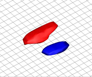
4.2. Quadrant analysis of the Reynolds shear stress
In this section, the statistical properties of the Reynolds shear stress  $-\bar {\rho }\widetilde {u''v''}$ are further investigated. The Reynolds shear stress is responsible for the energy exchange between mean shear flow and fluctuation components, and the wall-normal transportation of the streamwise momentum, which is the essential part of the turbulence generation process. Quadrant analysis for the Reynolds shear stress is a useful data-processing technique first proposed by Wallace et al. (Reference Wallace, Eckelmann and Brodkey1972). The quadrant analysis decomposes the products of the velocity fluctuations into the following four quadrant events in terms of the parameter plane of the velocity fluctuations of the streamwise (
 $u''$) and wall-normal (
 $v''$) components: Q1
  $(u''>0,\ v''>0)$, Q2
  $(u''<0,\ v''>0)$, Q3
  $(u''<0,\ v''<0)$ and Q4
  $(u''>0,\ v''<0)$. The Q2 and Q4 events are gradient-type motions and correspond to the ejection and sweep motions, respectively. The ejection is the fluid motion in that a near-wall low-momentum flow is lifted upward from the near-wall region and interacts with the high-momentum flow away from the wall. On the contrary, the sweep is the motion of a high-momentum flow going down toward the wall. The Q1 and Q3 events are counter-gradient-type motions contributing negatively to the Reynolds shear stress and called outward and inward interactions, respectively.
The results of applying the quadrant analysis to the present WMLES and DNS database are shown in figure 6. The ejection Q2 and the sweep Q4 events make the major contributions to the Reynolds shear stress, while the Q1 and Q3 events make fewer contributions to the total stress. Prior studies showed that the ejection Q2 makes the highest contributions to the Reynolds shear stress, excluding the very near-wall region, whereas, in the very close region to the wall  $(y^+\lesssim 12)$, the sweep (Q4) has the most (Wallace Reference Wallace2016). Figure 6 shows that this dominant feature of the Q2 is predicted by the WMLES although the WMLES does not resolve the small turbulent eddy dynamics in the near-wall region. The results indicate that the prediction capability of the balance among each quadrant event by the WMLES is favourable even in the near-wall region. The influence of Reynolds number effects is also observed at increasing Reynolds number. As for the ejection event (Q2), the WMLES agrees well with the DNS above the matching location at the lowest
  $Re_\tau \approx 700$ case. On the other hand, at increasing Reynolds number, under-predictions are observed at higher
  $Re_\tau \approx 1250$ and 2300. In the region below the matching location, the ejection (Q2) peak at
  $y^+\approx 40$ is not captured even at the lowest
  $Re_\tau \approx 700$. The sweep event (Q4) has similar tendencies where under-predictions appear at increasing Reynolds number, while the WMLES compares well with the DNS above the matching location at the lowest
  $Re_\tau \approx 700$. These results indicate that each decomposed quadrant event has some discrepancies from the DNS even above the matching location, although the total Reynolds shear stress is predicted correctly by the WMLES because of the shear-stress balance in the inner layer, as shown in the previous § 4.1. The quadrant analysis will be further investigated, and the structures and spatial relationships of the Q2 and Q4 quadrant events are revealed in the subsequent § 5. The predictability of the Reynolds number effects in the WMLES is also further discussed concerning the Reynolds normal stresses and the energy spectrum of the streamwise velocity fluctuations in § 6.

Figure 6. Quadrant analysis of the Reynolds shear stress  $-\bar {\rho }\widetilde {u''v''}$ at (a)
  $Re_\tau \approx 700$, (b)
  $Re_\tau \approx 1250$, (c)
  $Re_\tau \approx 2300$. Green, Q1
  $(u''>0,v''>0)$; blue, Q2
  $(u''<0,v''>0)$, black, Q3
  $(u''<0,v''<0)$; red, Q4
  $(u''>0, v''<0)$. Circles, DNS; lines, WMLES (solid, above the matching location; dash-dotted, below the matching location).
4.3. Turbulence kinetic energy budget
To investigate the near-wall turbulence generation in the WMLES from the statistical point of view, the budget of the TKE  $\tilde {k}=(1/2)\widetilde {u_i''u_i''}$ predicted by the WMLES is compared with that of the DNS database. The TKE budget equation for the compressible flow is written here as follows according to Kawai (Reference Kawai2019):
 \begin{equation} \frac{\partial \bar{\rho}\tilde{k}}{\partial t} ={-}C + P + T_d + T_p + D_v + D_d + M + \varPi_d, \end{equation}
where  $C$,
$C$,  $P$,
$P$,  $T_d$,
  $T_p$,
  $D_v$,
  $D_d$,
  $M$ and
  $\varPi _d$ on the right-hand side are the contributions from the convection, production, turbulent diffusion, velocity–pressure interaction, viscous diffusion, energy dissipation, mass flux contribution associated with density fluctuations and pressure dilatation, respectively, and each term is written as follows:
 \begin{equation} \left.\begin{gathered} C=\frac{\partial}{\partial x_j}(\bar{\rho}\widetilde{u_j}\tilde{k}),\quad P={-}\bar{\rho}\widetilde{u_i''u_j''}\frac{\partial \widetilde{u_i}}{\partial x_j}, \\ T_d={-}\frac{\partial}{\partial x_j}( \bar{\rho}\widetilde{u_i''u_i''u_j''}),\quad T_p={-}\frac{\partial}{\partial x_j}(\overline{p'u_j'}), \\ D_v=\frac{\partial}{\partial x_j}(\overline{\tau_{ij}'u_i'}),\quad D_d={-}\overline{\tau'_{ij}\frac{\partial u_i'}{\partial x_j}},\\ M=\overline{u_i''}\left( \frac{\partial \overline{\tau_{ij}}}{\partial x_j}-\frac{\partial \bar{p}}{\partial x_i}\right),\quad \varPi_d=\overline{p'\frac{\partial u_i'}{\partial x_i}}, \end{gathered}\right\} \end{equation}
where the modelled (SGS) stress in the WMLES is included in the stress term  $\tau _{ij}$. Figure 7(a–c) compares the budget terms,
  $C$,
$C$,  $P$,
$P$,  $T_d$,
  $T_p$,
  $D_v$ and
  $D_d$, which are normalized using the wall-shear stress and local viscous coefficient
  $\overline {\tau _w}^2/\bar {\mu }$. The mass flux contribution
  $M$ and pressure dilatation
  $\varPi _d$ are not shown because they are negligibly small in the present calculation condition. Each budget term obtained by the WMLES shows discrepancies from the DNS in the near-wall region below the matching location (represented by a dash-dotted line). On the other hand, the budget terms above the matching location (represented by a solid line) compare relatively well with the DNS, and reproduce the balance among each term. The production term
  $P$ has its peak at
  $y^+\approx 12$, and at the lowest
  $Re_\tau \approx 700$ (figure 7a), the near-wall peak is largely captured by the WMLES. However, at the highest
  $Re_\tau \approx 2300$ (figure 7c), the peak is hardly reproduced because of the lack of grid points in the near-wall region (the first grid point is already at
  $y_1^+\approx 16$), which implies that near-wall physical streaks driving the near-wall turbulence generation are not resolved on the computational grid at this high Reynolds number. Figure 7(d) represents the premultiplied production terms
  $y^+ P$ to investigate the dependence on the Reynolds numbers. There exist near-wall peaks at
  $y^+\approx 15$ and the profiles in the near-wall region are independent of the Reynolds numbers in the cases of the DNS, and the plateau region appears in the logarithmic region (
 $y^+\gtrsim 50$). On the other hand, the WMLES does not capture the near-wall peak, while good agreements with the DNS are observed in the logarithmic region above the matching location. It should be noted that, at
  $Re_\tau \approx 1250$ and
  $Re_\tau \approx 2300$, the second point off the wall shows a peak although the grid resolutions are insufficient to resolve the near-wall streaks. The production terms below the matching location imply the existence of the near-wall turbulence structures related to the turbulence generation in the WMLES, and the details are investigated in the next section.

Figure 7. (a–c) Show TKE budget terms at (a)  $Re_\tau \approx 700$, (b)
  $Re_\tau \approx 1250$ and (c)
  $Re_\tau \approx 2300$, respectively. Cyan, convection; red, production; black, turbulent diffusion; magenta, velocity–pressure interaction; green, viscous diffusion; blue, energy dissipation.
  $(d)$ Shows the comparison of the production terms premultiplied by normalized distance
  $y^+P$. Red,
  $Re_\tau \approx 700$; green,
  $Re_\tau \approx 1250$; blue,
  $Re_\tau \approx 2300$. Circles, DNS; lines, WMLES (solid, above the matching location; dash-dotted, below the matching location).
5. Near-wall turbulence structures and generation in the WMLES
As shown in the previous section, the statistical TKE production exists in the near-wall region below the matching location in the WMLES although the production peak is not sufficiently resolved on the computational grid. However, that is the time-averaged turbulence production, and the hydrodynamic events driving the near-wall turbulence generation are still unclear. Therefore, in this section, the instantaneous near-wall turbulence structures are first shown to confirm the differences between the WMLES and the DNS. Subsequently, a conditional-averaging technique for the instantaneous flow fields is applied to reveal the statistical properties of the near-wall turbulence structures, and the near-wall turbulence generation in the WMLES is discussed.
5.1. Instantaneous near-wall turbulence structures
Figures 8 and 9 show the streamwise velocity fluctuations  $u''$ on the cross-sections normal to the streamwise
  $(x=30.0\delta _0)$ and wall-normal
  $(y^+\approx 15)$ directions, respectively, where
  $y^+\approx 15$ is approximately the height of the maximum TKE production in the DNS as shown in figure 7. The instantaneous streamwise velocity fluctuation is normalized by the friction velocity
  $\overline {u_\tau }$, where
  $\overline {u_\tau }$ is calculated from the wall-shear stress averaged temporally and spatially in the spanwise direction at
  $x=30\delta _0$. From the results of the DNS (a, c and e of figures 8 and 9), the near-wall streaks; low- and high-speed regions located side by side exist and become smaller in size as the Reynolds number increases. On the other hand, the WMLES (b, d and f of figures 8 and 9) shows the different tendencies in the near-wall region, and suggests that differences between the WMLES and the DNS get more noticeable at increasing Reynolds number. At the lowest case
  $Re_\tau \approx 700$, the WMLES (b of figures 8 and 9) show relatively similar streamwise velocity fluctuations to the DNS (a of figures 8 and 9), i.e. the length scales of the turbulence structures look similar, which is most likely because the grid resolution for the WMLES is relatively close to that for the DNS. However, the comparisons between (c) and (d) or (e) and ( f) in figures 8 and 9, represent the turbulence structures with different length scales in the near-wall region, i.e. the length scales in the WMLES are larger than those in the DNS.

Figure 8. Instantaneous streamwise velocity fluctuations at the cross-section  $x=30\delta _0$; (a) DNS
  $(Re_\tau \approx 700)$, (b) WMLES
  $(Re_\tau \approx 700)$, (c) DNS
  $(Re_\tau \approx 1250)$, (d) WMLES
  $(Re_\tau \approx 1250)$, (e) DNS
  $(Re_\tau \approx 2300)$, ( f) WMLES
  $(Re_\tau \approx 2300)$. The region is
  $0.8\delta _0$ in the wall-normal (
 $y$) direction and
  $2.0\delta _0$ in the spanwise (
 $z$) direction.

Figure 9. Instantaneous streamwise velocity fluctuations on the wall-parallel plane at  $y^+\approx 15$. (a) DNS
  $(Re_\tau \approx 700)$, (b) WMLES
  $(Re_\tau \approx 700)$, (c) DNS
  $(Re_\tau \approx 1250)$, (d) WMLES
  $(Re_\tau \approx 1250)$, (e) DNS
  $(Re_\tau \approx 2300)$, ( f) WMLES
  $(Re_\tau \approx 2300)$. The region is
  $15.0\delta _0$ (
 $25.0\delta _0 < x < 40.0\delta _0$) in the streamwise (
 $x$) direction and
  $6.0\delta _0$ in the spanwise (
 $z$) direction.
To investigate the quantitative spanwise length scale of the near-wall turbulence structures, figure 10 shows the spanwise premultiplied energy spectra  $k_z \varPhi _{u''u''}$ of the streamwise velocity fluctuations
  $u''$ at
  $y^+\approx 15$, where
  $k_z$ is a wavenumber in the spanwise direction; (a) is plotted in terms of the wall unit spanwise wavelength
  $\lambda _z^+$ and (b) is
  $\delta$ unit
  $\lambda _z/\delta$. As shown in the previous study by Smith & Metzler (Reference Smith and Metzler1983), the average spanwise length of the near-wall streaks is
  $z^+\approx 100$ in the buffer region, and the results of the present DNS (circles) in figure 10(a) are consistent since the spectral peaks appearing at
  $\lambda _z^+\approx 100$. The energy spectra of the DNS collapse regardless of the Reynolds number, which demonstrates the near-wall turbulence structures in the DNS are scaled with wall units (
 $+$) non-dimensionalized by the viscous length scale
  $\delta _\nu$. On the other hand, the near-wall length scales in the WMLES are larger than those in the DNS, which indicates that larger turbulence structures exist in the near-wall region and is consistent with figures 8 and 9. Figure 10(a) shows that the spanwise length scale in the WMLES is not scaled with the viscous length scale
  $\delta _\nu$, whereas the spectra have their peaks almost at the same length scale if plotted in terms of the outer-layer length scale
  $\delta$, as shown in figure 10(b). These results imply that the near-wall spanwise length scale of the turbulence structures in the WMLES is determined by factors that are different from the near-wall flow physics confirmed in experiments and the DNS.

Figure 10. Premultiplied energy spectra of the streamwise velocity fluctuations at  $y^+\approx 15$; (a) wall units, (b)
  $\delta$ units. Red,
  $Re_\tau \approx 700$; green,
  $Re_\tau \approx 1250$; blue,
  $Re_\tau \approx 2300$. Circles, DNS; lines, WMLES.
To confirm the trends at higher Reynolds numbers, figure 11 shows the instantaneous streamwise velocity fluctuations at  $Re_\tau \approx 4100$, 7800 and 14 000 where there are no DNS data available. It should be noted that (b), (d) and ( f) in figure 11 show the wall-parallel plane at the first grid point off the wall (first grid point off the wall is already
  $y_1^+>15$, i.e.
  $y_1^+\approx 30$, 58 and 109 for
  $Re_\tau \approx 4100$, 7800 and 14 000, respectively). Even at these high Reynolds numbers, the near-wall low- and high-speed streaky structures are observed in the near-wall region (figure 11a,c,e), however, the length scales seem to be universal regardless of the increasing Reynolds number, unlike the DNS. The details of the near-wall turbulence structures in the WMLES are further investigated through the elucidation of the statistical properties in the next subsection.

Figure 11. Instantaneous streamwise velocity fluctuations for high Reynolds number cases. Cross-section at  $x=30\delta _0$, (a)
  $Re_\tau \approx 4100$, (c)
  $Re_\tau \approx 7800$, (e)
  $Re_\tau \approx 14\,000$. Wall-parallel plane at first grid point off the wall, (b)
  $Re_\tau \approx 4100$, (d)
  $Re_\tau \approx 7800$, ( f)
  $Re_\tau \approx 14\,000$. The region is the same as figures 8 and 9, respectively.
5.2. Statistical near-wall turbulence structures
A conditional-averaging technique is applied to the instantaneous flow fields to elucidate the statistical properties of the near-wall turbulence structures in the WMLES. As explained in § 4.3, the production term in the TKE budget equation is the product of the mean shear and the Reynolds stress. Therefore, to reveal the stress-bearing turbulence structures, the quadrant events investigated in § 4.2 are further considered. The present procedure of the conditional averaging for quadrant events is based on the generalization to three-dimensional structures first conducted by Lozano-Durán, Flores & Jiménez (Reference Lozano-Durán, Flores and Jiménez2012). Based on their procedure, some minor modifications are made for applying the technique to the present calculation settings. The detailed procedures are explained first, and subsequently, the conditionally averaged near-wall turbulence structures are shown.
5.2.1. Filtering parameter for intense quadrant events
To detect the statistical properties of the intense structures mostly contributing to the Reynolds shear stress, the intense quadrant events to extract are defined as follows:
 \begin{equation} |u''v''(y)|>Hu_{rms}(y) v_{rms}(y), \end{equation}
where  $u''v''(y)$ is the instantaneous point-wise Reynolds shear stress at height
  $y$,
$y$,  $u_{rms}(y)$ and
  $v_{rms}(y)$ are the root-mean-squares of
  $u$ and
  $v$, respectively, and
  $H$ is the hyperbolic-hole parameter (Willmarth & Lu Reference Willmarth and Lu1972). The right-hand side of (5.1) represents the threshold depending on the wall distance
  $y$, and the hole parameter
  $H$ determines the hyperbolic-hole size, i.e. the intense components of the Reynolds stress are defined as the magnitude of the velocity fluctuation
  $|u''v''|$ outside of the hyperbolic hole.
The detection of the turbulence structures based on the quadrant analysis depends largely on the hyperbolic-hole size  $H$. In previous studies, the value
  $H=1.75$ has often been employed (e.g. Lozano-Durán et al. Reference Lozano-Durán, Flores and Jiménez2012; Jiménez Reference Jiménez2018), and the same value is employed in this study. The dependence of the intense Reynolds shear stress on the parameter
  $H$ for the DNS and the WMLES is investigated. Figure 12 shows the contributions to the Reynolds shear stress from each quadrant event at
  $y^+=15$ as a function of the parameter
  $H$ for the present DNS and WMLES. Figure 12 also includes the frequency of occurrence (cyan circles) and Reynolds shear stress lying inside the hole (grey solid lines). When
  $H=1.75$ is chosen (represented by the vertical dotted line), approximately 55 % of the total Reynolds shear stress resides outside the hole, whereas the frequency of occurrence outside the hall is less than 10 % in both the DNS and the WMLES. The Reynolds shear stress lying outside the hole consists of mostly Q2 (ejection) and Q4 (sweep) events, each still accounting for approximately 30 %–40 % of the total Reynolds stress, and much smaller contributions from the counter-gradient Q1 and Q3 events. It should be noted that both the DNS and the WMLES represent similar profiles, while slight differences are observed when the parameter
  $H$ is small. In conclusion, the hole parameter
  $h=1.75$ is appropriate to detect the quadrant events contributing mostly to the intense Reynolds stress events for both the DNS and the WMLES, and the conditional averaging using this parameter value is conducted in the subsequent sections.

Figure 12. Fractional contributions to the total Reynolds shear stress by each quadrant event lying outside the hole as a function of the magnitude filtering parameter  $H$ at the height of
  $y^+\approx 15$. The profiles are calculated from the results at
  $Re_\tau \approx 2300$; (a) DNS, (b) WMLES. Green, Q1; blue, Q2; black, Q3; red, Q4; grey lines; all quadrant values lying inside the hole. Symbol (cyan open circle), frequency of occurrence of the quadrant event inside the hole.
5.2.2. Procedures of the conditional averaging
The quadrant analysis is extended to three-dimensional connected structures by Lozano-Durán et al. (Reference Lozano-Durán, Flores and Jiménez2012), and it is shown that the typical and dominant ensemble-averaged structures in the logarithmic region are side-by-side Q2 (ejection) and Q4 (sweep) pairs separated by a quasi-streamwise vortex. In the present study, we focus on the near-wall turbulence structures, and thus a conditional-averaging technique with minor modifications from Lozano-Durán et al. (Reference Lozano-Durán, Flores and Jiménez2012) is applied to the instantaneous flow fields to detect the statistical structures of the Q2 and Q4 in the near-wall region. To obtain the statistical structures, the instantaneous flow fields are ensemble averaged under the condition of the concurrent presence of the Q2 and Q4 as a pair, and the details of the averaging procedure are as follows.
The searching area of the quadrant pair is shown in figure 13. First, a Q2 (ejection) event at the height of  $y^+=15$ is searched in the spanwise direction on the cross-section
  $x=30.0\delta _0$. If a Q2 event is detected at a certain location, further detection for the concurrent neighbouring Q4 (sweep) events is followed. The spanwise detection range for the Q4 is determined as the length scale of the spanwise energy spectrum peaks confirmed in figure 10, i.e.
  $z_s^+<100$ for the DNS and
  $z_s/\delta <0.2$ for the WMLES. The vertical detection range is set to between half and twice the height of the detected Q2, i.e.
  $7.5< y^+<30$, having a range referring to Lozano-Durán et al. (Reference Lozano-Durán, Flores and Jiménez2012). The Q4 events existing inside the searching area are counted as the pair of the first detected Q2, and the instantaneous flow fields are averaged in the following reference frame:
 \begin{equation} \boldsymbol{r}=\boldsymbol{x}-\boldsymbol{x}_{centre}, \end{equation}
where  $\boldsymbol {x}=(x,y,z)$ is the original coordinate of the instantaneous flow field,
  $\boldsymbol {x}_{centre}=(x,y,z_{centre})$ is the spanwise midpoint of the line connecting the detected Q2 and Q4 pair and
  $\boldsymbol {r}$ is the relative coordinate used for conditional averaging. It should be noted that the present averaging procedure is conducted under the condition that Q2 is first detected and neighbouring Q4 exists concurrently, however, equivalent results are obtained when the Q2–Q4 pair is defined as a Q4 with a neighbouring Q2, and there is no crucial difference depending on the detection order of the pair, although not shown in this paper. Another point that should be noted is the detection height for the WMLES. There is no sufficient grid resolution in the near-wall region in the WMLES, therefore, the height
  $y^+\approx 15$ used for the detection of Q2 is a few grid points off the wall; the third grid point off the wall at
  $Re_\tau \approx 700$ (
 $y_3^+=14.3$), second grid point at
  $Re_\tau \approx 1250$ (
 $y_2^+=17.5$) and first grid point at
  $Re_\tau \approx 2300$ (
 $y_1^+=16.2$), respectively.

Figure 13. Schematic of the searching area for the Q2–Q4 pair.
5.3. Conditionally averaged turbulence structures
Figure 14 shows the conditionally averaged streamwise velocity fluctuations  $\widehat {u''}/\overline {u_\tau }$ at the cross-section (
 $x=30.0\delta _0$), where the value
  $\hat {\phi }$ represents the conditionally averaged quantities of
  $\phi$ and the grids are superimposed only in the results of the WMLES to specify the grid resolution. As indicated in the instantaneous streamwise velocity fluctuations (figure 8), at the lowest
  $Re_\tau \approx 700$, the length scale in the WMLES is quite similar to that of the DNS. However, as the Reynolds number increases, the differences between the DNS and the WMLES become more noticeable, since the spanwise length scales in the WMLES are almost constant regardless of the increasing Reynolds number, unlike the DNS. It should be noted that the computational grid used in the WMLES is intentionally designed such that the grid does not resolve the near-wall viscous-scaled structures sufficiently. Although the length scales are non-physically elongated, the typical streak-like structures, i.e. side-by-side Q2–Q4 pairs, are observed in the WMLES. The spanwise length scale between the centres of the Q2 and Q4 pair is approximately 4 grid points for all Reynolds numbers, i.e. approximately 8 grid points in one spanwise wavelength
  $\lambda _z$. The results correspond well to the spanwise energy spectra of the streamwise velocity fluctuations shown in figure 10(b), where the spectra are scaled with the boundary-layer thickness
  $\delta$. It should be noted that the conditionally averaged streamwise velocity fluctuations at higher Reynolds numbers
  $Re_\tau \approx 4100$, 7800 and 14 000 in the WMLES show similar statistical properties to that at
  $Re_\tau \approx 2300$, as expected from the instantaneous streamwise velocity fluctuations (figures 8f, 9f, 11); see Appendix B for further details.

Figure 14. Conditionally averaged streamwise velocity fluctuations of the Q2–Q4 pair on the cross-section ( $x=30.0\delta _0$); (a) DNS
  $(Re_\tau \approx 700)$, (b) WMLES
  $(Re_\tau \approx 700)$, (c) DNS
  $(Re_\tau \approx 1250)$, (d) WMLES
  $(Re_\tau \approx 1250)$, (e) DNS
  $(Re_\tau \approx 2300)$, ( f) WMLES
  $(Re_\tau \approx 2300)$. The computational grid is superimposed in the results of the WMLES. The region is
  $0.32\delta _0$ in the wall-normal (
 $y$) direction and
  $0.6\delta _0$ in the spanwise (
 $z$) direction.
Figure 15 shows the three-dimensional turbulence structures of the conditionally averaged Q2 and Q4 pairs. The isosurfaces of the streamwise velocity fluctuations at  $\widehat {u''}/u_\tau =-1.5$ for Q2 (blue objects) and
  $\widehat {u''}/\overline {u_\tau }=1.5$ for Q4 (red objects) are shown, and it should be noted the Q2 and Q4 structures correspond to the low- and high-speed streaks, respectively. Interestingly, the three-dimensional Q2–Q4 coherent structures are obtained even in the case of the WMLES, which indicates the near-wall region in the WMLES is not spatially disordered, although the near-wall physical coherent structures are not intentionally resolved in the WMLES. The Q4 structures are larger than Q2, while the difference is relatively small in the WMLES compared with the DNS, especially at high Reynolds numbers. It is mentioned by Jiménez (Reference Jiménez2018) that the high-velocity streak (Q4) is larger than the low-velocity streak (Q2) when conditionally averaged by Q2–Q4 pairs because the motions of the high-speed regions caused by the sweep (Q4) are fed from the region away from the wall, while the motions of the low-speed regions caused by the ejection (Q2) are blocked by the wall. At the lowest Reynolds number
  $Re_\tau \approx 700$, the length scale of the Q2–Q4 structures obtained by the WMLES is quite similar to those obtained by the DNS three-dimensionally. On the other hand, the streak-like structures obtained by the WMLES are non-physically elongated in the spanwise directions compared with those obtained in the DNS, at increasing Reynolds number. Furthermore, the conditionally averaged three-dimensional near-wall turbulence structures at higher Reynolds numbers
  $Re_\tau \approx 4100$, 7800 and 14 000 in the WMLES also show similar statistical properties to that at
  $Re_\tau \approx 2300$ (see Appendix B). It should be noted that the near-wall turbulence structures in the WMLES could depend heavily on the computational grid and the numerical method due to the coarse grid resolution. Therefore, additional cases varying the grid resolutions and numerical methods (numerical schemes and SGS models) were also conducted to confirm the consistency of the present conclusions (see Appendices C and D for the sensitivity of the statistical near-wall turbulence structures to the grid resolutions and numerical methods, respectively). The dominant factor to determine the length scale of the near-wall turbulence structures in the WMLES is further investigated in the next § 5.4.

Figure 15. Conditionally averaged near-wall three-dimensional turbulence structures of the Q2–Q4 pair. Blue iso-surface, Q2 (low-speed streaks); red iso-surface, Q4 (high-speed streaks). The iso-surfaces are defined at  $\widehat {u''}/\overline {u_\tau }=-1.5$ for Q2, and
  $\widehat {u''}/\overline {u_\tau }=1.5$ for Q4. (a) DNS (
 $Re_\tau \approx 700$), (b) WMLES (
 $Re_\tau \approx 700$), (c) DNS (
 $Re_\tau \approx 1250$), (d) WMLES (
 $Re_\tau \approx 1250$), (e) DNS (
 $Re_\tau \approx 2300$), ( f) WMLES (
 $Re_\tau \approx 2300$). The grid spacing shown at the wall is 0.05
 $\delta _0$ in both the streamwise (
 $x$) and spanwise (
 $z$) directions.
The fundamental question of why wall-bounded turbulent flows can sustain themselves has been studied over several decades (Jiménez & Moin Reference Jiménez and Moin1991; Hamilton et al. Reference Hamilton, Kim and Waleffe1995; Jiménez & Pinelli Reference Jiménez and Pinelli1999; Kawahara & Kida Reference Kawahara and Kida2001; Panton Reference Panton2001), and one consensus is that the near-wall turbulence coherent structures, i.e. low- and high-speed streaks, contribute to the self-sustaining mechanism of the turbulence, although there is room for further discussions on the detailed mechanisms such as inner–outer-layer interactions. In general, coherent streaky structures are regarded as organized motions that are persistent in time and space, and the self-sustaining process based on the instability and transitional growth of the streaks is as follows: the low-speed streaks are unstable because the low-speed regions are surrounded by the high-speed regions, i.e. inflection points exist in the spanwise velocity distributions between the low- and high-speed streaks. If perturbations are added to these structures, the nonlinear development of the transient-growth mode causes the abrupt eruption of the low-speed fluid, which is called bursting, and induces quasi-streamwise vortices. The quasi-streamwise vortices take away the energy from the mean flow and produce new streaks, and the processes are repeated as each process is discussed by Kim et al. (Reference Kim, Kline and Reynolds1971), Blackwelder & Eckelmann (Reference Blackwelder and Eckelmann1979), Swearingen & Blackwelder (Reference Swearingen and Blackwelder1987), Waleffe (Reference Waleffe1997), etc. Therefore, the existence of the near-wall streak-like coherent structures which are composed of the adjacent low- and high-speed regions (Q2–Q4 pairs) elucidated in the present study is evidence of the generation of the quasi-streamwise vortices and the existence of the near-wall turbulence generation in the WMLES, while the length scales of the coherent structures are non-physically elongated. Figure 16 shows the conditionally averaged streamwise velocity fluctuations obtained by the WMLES, which is superimposed by the cross-section streamlines and shows the spatial relationship of the streamwise vortex and the low- (Q2) and high- (Q4) speed regions, where the Q2 and Q4 regions are on either side of the streamwise vortex. Although the near-wall coherent structures in the present WMLES are not elongated in the streamwise direction compared with the spanwise direction unlike those observed in the DNS (see figure 15), Jiménez (Reference Jiménez2022) shows recently that there are turbulence states in which bursting takes place without long structures of the streamwise velocity. Therefore, present results in the WMLES also support the idea proposed by Jiménez (Reference Jiménez2022) that typical streaks elongated in the streamwise direction are not necessarily required for the self-sustaining process of the wall-bounded turbulence.

Figure 16. Cross-section streamlines computed from  $(\hat {v},\hat {w})$ at
  $x=30.0\delta _0$ superimposed on the conditionally averaged streamwise velocity fluctuations obtained by the WMLES at
  $Re_\tau \approx 2300$ (same as figure 14f).
In summary, the most important finding obtained in the present section is that the near-wall region of the WMLES is not composed of disordered random structures, but streak-like coherent structures, although the near-wall region below the matching location is not intentionally resolved on the typical computational grid in the WMLES, and it is suggested that the near-wall turbulence generation in the WMLES is maintained by the numerically elongated near-wall coherent structures.
5.4. Length scale of the near-wall turbulence structures in the WMLES
From the results of the spanwise energy spectra in figure 10 and the conditional-averaging results in figures 14 and 15, the length scales of the near-wall coherent structures in the WMLES are not scaled with the typical viscous length  $\delta _\nu$. To confirm the convergence trend of the spanwise length scale of the near-wall turbulence structures in the WMLES, figure 17(a) shows the spanwise correlation of the streamwise velocity fluctuation
  $R_{u''u''}$ at
  $y^+\approx 15$, where the results at higher Reynolds numbers
  $Re_\tau \approx 4100$, 7800 and 14 000 are also included. At
  $Re_\tau \approx 4100$, 7800 and 14 000, the spanwise correlations are calculated at the first grid points off the wall since there is no grid point in the near-wall region
  $y^+\lesssim 15$, as described in § 5.1. The length scales of spanwise wavelength are almost constant at all Reynolds numbers, which indicates that the length scales of the near-wall turbulence structures in the WMLES are influenced by the insufficient grid resolution in the near-wall region. To investigate the scaling factor to determine the spanwise length scale of the near-wall turbulence structures in the WMLES, the following three scalings are considered in the present study: (i) typical wall-unit scaling, (ii) semi-local scaling (Coleman, Kim & Moser Reference Coleman, Kim and Moser1995) and (iii) semi-local scaling with SGS eddy viscosity. The first scaling using the physical quantities at the wall is the typical scaling for wall-bounded turbulent flows. As already described, the viscous length
  $\delta _\nu$ in this scaling is represented as
 \begin{equation} \delta_\nu=\frac{\nu_w}{u_\tau}=\frac{\mu_w}{\rho_w u_\tau},\quad u_\tau=\sqrt{\frac{\tau_w}{\rho_w}}. \end{equation}
In the second semi-local scaling, the viscous length  $\delta _\nu ^*$ is defined by using the local quantities
  $\rho$ and
  $\mu$ at height
  $y$ (Coleman et al. Reference Coleman, Kim and Moser1995)
 \begin{equation} \delta_\nu^*=\frac{\nu}{u_\tau^*}=\frac{\mu}{\rho u_\tau^*},\quad u_\tau^*=\sqrt{\frac{\tau_w}{\rho}}. \end{equation}
In the third scaling, we add the SGS eddy viscosity  $\mu _{t,sgs}$ to the physical viscosity of the above semi-local scaling to take into account the effects of the eddy viscosity
  $\mu _{t,sgs}$ on the near-wall turbulence length scale
 \begin{equation} \delta_{\nu}^{*,sgs}=\frac{\nu+\nu_{t,sgs}}{u_\tau^*}=\frac{\mu+\mu_{t,sgs}}{\rho u_{\tau}^*}. \end{equation}
Figure 17(b) shows the spanwise length scale of the near-wall turbulence structures non-dimensionalized by the three viscous length scales  $\delta _\nu, \delta _\nu ^*,\ \delta _{\nu }^{*,sgs}$. The spanwise length scale non-dimensionalized with wall-unit scaling (
 $l_z^+$, red symbols) and semi-local scaling (
 $l_z^*$, green symbols) represents almost linear increases at increasing Reynolds number. On the other hand, the spanwise length scale non-dimensionalized with the semi-local scaling including SGS eddy viscosity (
 $l_z^{*,sgs}$, blue symbols) represents an almost collapsed value, and the normalized length
  $l_z^{*,sgs}$ is the same order as the typical wall-unit-scaled spanwise length scale confirmed in experiments and the DNS;
  $l_z^+\sim O(100)$ in the buffer region (Smith & Metzler Reference Smith and Metzler1983), which indicates that the diffusion introduced by the SGS eddy viscosity dominantly determines the spanwise length scale of the numerical turbulence structures in the WMLES. We have confirmed that the proposed semi-local scaling including SGS eddy viscosity is consistently effective regardless of the grid resolutions, numerical schemes (low-pass filtering) and SGS models (see Appendices C and D for further details, respectively).

Figure 17. The spanwise length scale of the near-wall turbulence structures in the WMLES. (a) spanwise correlation of the streamwise velocity fluctuations. Red,  $Re_\tau \approx 700$; green,
  $Re_\tau \approx 1250$; blue,
  $Re_\tau \approx 2300$, magenta,
  $Re_\tau \approx 4100$; cyan,
  $Re_\tau \approx 7800$; black,
  $Re_\tau \approx 14\,000$. (b) The spanwise length scale of the near-wall turbulence structures non-dimensionalized with three different viscous length scales. Red, wall-unit scaling; green, semi-local scaling (Coleman et al. Reference Coleman, Kim and Moser1995); blue, semi-local scaling including SGS eddy viscosity.
6. Predictability of Reynolds number effects in the WMLES
In contrast to the previous discussions on near-wall turbulence, the logarithmic region is focused on in the present section. The outer peak is known to appear in the logarithmic region in the energy spectrum of the streamwise velocity fluctuations at increasing Reynolds number (Marusic et al. Reference Marusic, Mathis and Hutchins2010a). However, the predictability of the outer peak in the WMLES has not been addressed. Therefore, the predictability of the outer peak by the WMLES and its origin are discussed because the outer peak is likely to be related to the near-wall turbulence structures and generation through inner–outer-layer interactions.
6.1. Reynolds normal stresses
As already shown in § 4.1, the mean streamwise velocity  $\bar {u}_{vD}$ and the Reynolds shear stress
  $-\bar {\rho }\widetilde {u''v''}$ predicted by the WMLES compare well with the DNS above the matching location, since the underlying assumption of the inner-layer modelling, i.e. the total shear-stress balance in the inner layer, is strictly satisfied (Kawai & Larsson Reference Kawai and Larsson2012). On the other hand, the predictability of the Reynolds normal stresses,
  $\bar {\rho } \widetilde {u''u''}$,
  $\bar {\rho } \widetilde {v''v''}$ and
  $\bar {\rho } \widetilde {w''w''}$, in the WMLES, is not derived from the total shear-stress balance. By both the experimental and numerical simulation studies conducted in the past, it is revealed that the Reynolds normal stresses represent relatively strong Reynolds number effects (Marusic et al. Reference Marusic, Mathis and Hutchins2010a). Substantial efforts have been devoted to elucidating the scaling behaviours of the streamwise Reynolds normal stress
  $\bar {\rho } \widetilde {u''u''}$ as well as to the other components,
  $\bar {\rho } \widetilde {v''v''}$ and
  $\bar {\rho }\widetilde {w''w''}$ (e.g. De Graaff & Eaton Reference De Graaff and Eaton2000; Hoyas & Jiménez Reference Hoyas and Jiménez2006). It is argued that the streamwise and spanwise components do not follow the wall-unit scaling, while the wall-normal component almost does (Marusic et al. Reference Marusic, Mathis and Hutchins2010a). The most noticeable feature is the increase in the streamwise component at increasing Reynolds numbers in the near-wall region (
 $y^+\approx 15$) and the outer peak in the logarithmic region (around
  $y/\delta \approx 0.15$). The increase of the streamwise Reynolds normal stress in the logarithmic region corresponds to the appearance of the outer peak in the premultiplied energy spectrum of the streamwise velocity fluctuations (Marusic et al. Reference Marusic, Mathis and Hutchins2010a,Reference Marusic, McKeon, Monkewitz, Nagib, Smits and Sreenivasanb; Smits et al. Reference Smits, McKeon and Marusic2011). The appearance of the outer peak is the criterion of the high Reynolds number for wall-bounded turbulent flows according to Smits et al. (Reference Smits, McKeon and Marusic2011) because the outer peak in the premultiplied energy spectrum starts to appear prominently only at sufficiently high Reynolds numbers, e.g.
  $Re_\tau \gtrsim 1700$, in contrast to the universal inner peak at
  $y^+\approx 15$ where the production peak of the near-wall turbulence appears. Bose & Park (Reference Bose and Park2018) discussed that the inner peak at
  $y^+\approx 15$ is inevitably under-resolved in the WMLES by its nature and that the outer peak is also likely to be under-resolved in the WMLES. To our knowledge, however, it has never been addressed whether the WMLES captures the appearance of the outer peak at increasing Reynolds number.
Figure 18 shows the Reynolds normal stresses obtained by the WMLES and the DNS. It is observed that there are relatively large differences between the WMLES and the DNS in the streamwise components even above the matching location away from the wall  $(y/\delta \gtrsim 0.085)$ as the Reynolds number increases to
  $Re_\tau \approx 1250$ and 2300, while the WMLES agrees reasonably well with the DNS at the lowest
  $Re_\tau \approx 700$. On the other hand, spanwise and wall-normal components obtained by the WMLES compare well with the DNS at all Reynolds numbers. It should be noted that similar predictions of the streamwise Reynolds normal stress by the WMLES were also observed in previous studies (e.g. Kawai & Larsson Reference Kawai and Larsson2012; Park & Moin Reference Park and Moin2014). From the DNS results in figure 18(a), the inner peak at
  $y^+ \approx 15$ of the streamwise component
  $\bar {\rho } \widetilde {u''u''}$ gradually increases at increasing Reynolds number. This is due to the superposition effects of the large-scale structures scaled with boundary-layer thickness as shown in the premultiplied energy spectra at
  $y^+\approx 15$ (see figure 10), which are represented by the increase of the low-frequency components at
  $\lambda _z/\delta \approx 1.0$ of figure 10(b) (vertical dashed line). Furthermore, it is confirmed that the streamwise Reynolds normal stress in the logarithmic region increases at increasing Reynolds number in the DNS, which suggests a failure of the wall-unit scaling in the logarithmic region, while the Reynolds normal stress obtained by the WMLES shows almost identical results regardless of the Reynolds number if plotted in terms of the wall distance scaled with the outer-layer length scale
  $y/\delta$ (see figure 18b).

Figure 18. Reynolds normal stresses obtained by the WMLES and the DNS; (a) wall unit, (b)  $\delta$ unit. From upper to lower, streamwise
  $\bar {\rho } \widetilde {u''u''}$, spanwise
  $\bar {\rho } \widetilde {w''w''}$ and wall-normal
  $\bar {\rho } \widetilde {v''v''}$ components, respectively. Red,
  $Re_\tau \approx 700$; green,
  $Re_\tau \approx 1250$; blue,
  $Re_\tau \approx 2300$. Circles, DNS; lines, WMLES (solid, above the matching location; dash-dotted, below the matching location).
Figure 19 shows the premultiplied spanwise energy spectra  $\varPhi _{u''u''}(y,\lambda _z)$ of the streamwise velocity fluctuations with the wall-unit scaling. The energy spectra obtained by the DNS show two distinct peaks (left column of figure 19). The inner peak corresponding to the near-wall streak is located at
  $y^+\approx 15$ at all Reynolds numbers. As the Reynolds number increases, the second outer peak starts to appear in the logarithmic region. On the other hand, in the cases of the WMLES, the inner peak exists at all Reynolds numbers, while the peak location is not the same as the DNS, which is explained by the different length scales of the near-wall turbulence structures in the WMLES as elucidated in the previous § 5. The outer peak does not appear clearly in the WMLES regardless of the increasing Reynolds number. Figure 20 shows the values of the energy spectra at
  $y/\delta \approx 0.15$ where the increase of the outer peak appears in the DNS. It should be noted that
  $y/\delta \approx 0.15$ corresponds to
  $y^+\approx 107$ at
  $Re_\tau \approx 700$,
  $y^+\approx 192$ at
  $Re_\tau \approx 1250$ and
  $y^+\approx 360$ at
  $Re_\tau \approx 2300$. The peaks that appear at
  $\lambda _z/\delta \approx 1.0$ are almost constant regardless of the Reynolds number in the WMLES, while the peaks in the DNS gradually increase at increasing Reynolds number. Figure 21 shows the instantaneous streamwise velocity fluctuations on the wall-parallel planes at
  $y/\delta \approx 0.15$ to investigate the difference in the instantaneous turbulence structures. According to Marusic et al. (Reference Marusic, Mathis and Hutchins2010a), the very long, meandering, large-scale structures consisting of the narrow regions of the low-momentum fluid flanked by higher-momentum fluid, called super-structures (Hutchins & Marusic Reference Hutchins and Marusic2007), develop at increasing Reynolds number, and it is argued that the super-structures contribute to the development of the outer peak, although the origins of the large-scale structures have not been revealed. Comparing the instantaneous turbulence structures of the WMLES with those of the DNS in figure 21, there is no noticeable difference at
  $y/\delta \approx 0.15$ in contrast to the structures at
  $y^+ \approx 15$ in the near-wall region (see figure 9). We have confirmed that the outer peak does not appear in the higher Reynolds number cases, and regardless of the numerical scheme (low-pass filtering) and the SGS model (see Appendices B and D for further details, respectively). To make the fluctuation components contributing to the increase of the outer peak clear, the length-scale decomposition of the streamwise velocity fluctuations is conducted in the next subsection.

Figure 19. Premultiplied spanwise energy spectra of streamwise velocity fluctuations  $k_z \varPhi _{u''u''}$; (a) DNS
  $(Re_\tau \approx 700)$, (b) WMLES
  $(Re_\tau \approx 700)$, (c) DNS
  $(Re_\tau \approx 1250)$, (d) WMLES
  $(Re_\tau \approx 1250)$, (e) DNS
  $(Re_\tau \approx 2300)$, ( f) WMLES
  $(Re_\tau \approx 2300)$.

Figure 20. Premultiplied spanwise energy spectra of streamwise velocity fluctuations at  $y/\delta \approx 0.15$ in terms of
  $\lambda _z/\delta$. Red,
  $Re_\tau \approx 700$; green,
  $Re_\tau \approx 1250$; blue,
  $Re_\tau \approx 2300$. Circles, DNS; lines, WMLES.

Figure 21. Instantaneous streamwise velocity fluctuations in the wall-parallel plane at  $y/\delta \approx 0.15$; (a) DNS
  $(Re_\tau \approx 700)$, (b) WMLES
  $(Re_\tau \approx 700)$, (c) DNS
  $(Re_\tau \approx 1250)$, (d) WMLES
  $(Re_\tau \approx 1250)$, (e) DNS
  $(Re_\tau \approx 2300)$, ( f) WMLES
  $(Re_\tau \approx 2300)$. The region is
  $15.0\delta _0$ (
 $25.0\delta _0 \le x \le 40.0\delta _0$) in the streamwise (
 $x$) direction and
  $6.0\delta _0$ in the spanwise (
 $z$) direction.
6.2. Length-scale decomposition of the streamwise Reynolds normal stress
To elucidate the reason for the appearance of the outer peak in the premultiplied energy spectrum and the deterioration of the predictability in the WMLES with increasing Reynolds number, the time-series data of the streamwise velocity fluctuations are decomposed into small and large length-scale contributions using a simple cutoff spectral filter in the spanwise direction as investigated by Marusic et al. (Reference Marusic, Mathis and Hutchins2010a). In the present study, the cutoff value  $\lambda _z/\delta =0.7$ is chosen to make the inner–outer-layer scale separation clear. Figure 22 shows the results of the streamwise Reynolds normal stress decomposed by the cutoff value. Figure 22(a) is the original results with all turbulence length scales, (b) is the results that are composed of only small length-scale components (
 $\lambda _z/\delta \leq 0.7$) and (c) is that with only large length-scale components (
 $\lambda _z/\delta >0.7$). As shown in figure 22(b), the results obtained by the WMLES (solid lines) agree well with the DNS (circles), which indicates that the WMLES reproduces the small turbulence fluctuations with the length scale of
  $\lambda _z/\delta \leq 0.7$. On the other hand, in figure 22(c), the WMLES does not predict the increase of the distributions observed in the DNS at increasing Reynolds number. The increase of the large length-scale components in the logarithmic region contributes to the outer peak observed in the premultiplied energy spectra (figure 19). The length-scale decomposition makes it clear that the deterioration of the outer peak predictability in the WMLES is attributed to the failure of the prediction of large-scale turbulent fluctuations. This result might be surprising because the computational grid used in the WMLES is designed to resolve the large energy-carrying vortices with the length scale of the boundary-layer thickness
  $\delta$ in the logarithmic and outer regions. The present results indicate that the large length-scale fluctuations of the order of
  $\delta$ are not properly predicted by the WMLES.

Figure 22. Length-scale decomposition of the streamwise velocity fluctuations. (a) All length scales (same as figure 18a), (b) only small length scales ( $\lambda _z/\delta \leq 0.7$), (c) only large length scales (
 $\lambda _z/\delta >0.7$). Red,
  $Re_\tau \approx 700$; green,
  $Re_\tau \approx 1250$; blue,
  $Re_\tau \approx 2300$. Circles, DNS; lines, WMLES (solid, above the matching location; dash-dotted, below the matching location).
Unfortunately, as far as we surveyed previous studies, the origin of the outer peak has not been revealed. Therefore, it is difficult to further discuss the cause of the deterioration of the outer peak predictability in the WMLES. However, one possible reason is the appearance of the outer peak could be associated with the increase of the inner peak through the inner–outer-layer interactions (Marusic et al. Reference Marusic, Baars and Hutchins2017; Mäteling & Schröder Reference Mäteling and Schröder2022; Zhou et al. Reference Zhou, Xu and Jiménez2022). As already described, the inner peak at  $y^+ \approx 15$ increases at increasing Reynolds number by the modulation effects of the outer large-scale components (Hutchins & Marusic Reference Hutchins and Marusic2007; Mathis et al. Reference Mathis, Hutchins and Marusic2009), and the WMLES does not resolve the inner peak due to the insufficient grid resolution there. The research that should be noted here is the wall-bounded turbulent flow simulations without walls conducted by Mizuno & Jiménez (Reference Mizuno and Jiménez2013). In their study, the DNS of turbulent channel flows where the inner layer is replaced by an off-wall boundary condition is performed. The off-wall boundary condition is synthesized from rescaled interior flow planes and imposed as a shifted copy within the logarithmic layer (at
  $y^+=130$). The mean streamwise velocity in the logarithmic region is successfully recovered by shifting the virtual walls although near-wall streaks are not resolved. Therefore, Mizuno & Jiménez (Reference Mizuno and Jiménez2013) conclude that the structures in the logarithmic region do not depend on seeding from the wall. However, in the present study, it is demonstrated that the predictability of some turbulence statistics such as the streamwise Reynolds normal stress by the WMLES deteriorates in the logarithmic region, which indicates that the turbulence dynamics of the near-wall inner layer has some influence on the large-scale eddy dynamics in the logarithmic region. If the Reynolds number effects of the inner and outer peaks interact with each other, it is reasonable to conclude that the WMLES cannot reproduce the increase of the outer peak correctly because of the failure of capturing the inner peak. Although the above discussion is just speculation as of now, the present results obtained by the WMLES indicate the possibility that the origin of the outer peak lies in the interaction with the inner peak corresponding to the streaks driving the near-wall turbulence generation, and the outer peak does not appear alone without resolving or correctly reflecting the near-wall turbulence structures.
7. Concluding remarks
In the present study, the near-wall turbulence structures in the WMLES were closely investigated by comparing with those of DNS, and it was revealed that there exist numerical coherent structures which are composed of low- and high-speed fluids alternating in the spanwise direction, while the length scale of the structures is non-physically elongated compared with those obtained by the DNS. Furthermore, it was revealed that the appearance of the outer peak, which is the Reynolds number effect in the energy spectrum of the streamwise velocity fluctuations, is not predicted by the WMLES.
In the quadrant analysis, the intense quadrant events contributing to the Reynolds shear stress generation are the ejection (Q2) and sweep (Q4) events, and the present results showed that the WMLES predicts their contributions even in the under-resolved near-wall regions. Concerning the TKE budget equation, it was shown that the production term exists in the under-resolved near-wall region of the WMLES, while they were not properly predicted due to the insufficient grid resolution. These facts implied the existence of the near-wall turbulence structures related to the turbulence generation in the WMLES.
To reveal the statistical near-wall turbulence structures, the instantaneous flow fields were averaged under the condition that intense quadrant events; the ejection (Q2) and the sweep (Q4) are located as side-by-side pairs concurrently, and the conditionally averaged flow fields elucidated the statistical properties of the near-wall turbulence structures in the WMLES. The important finding obtained by conditional averaging is that the near-wall turbulence structures in the WMLES are not disordered random structures, but coherent structures. The length scale of the near-wall turbulence structures in the WMLES was found to be non-physically elongated compared with the DNS, i.e. the length scale of the near-wall turbulence structures is not scaled by the typical viscous length defined by the friction velocity and the molecular viscosity at the wall. To clarify the scaling of the near-wall length scale in the WMLES, we proposed the semi-local scaling including the SGS eddy viscosity, and the proposed scaling revealed that the length scale of the near-wall coherent structures is elongated dominantly by the diffusion introduced by the SGS eddy viscosity. The spanwise length scale of the near-wall turbulence structures normalized by the proposed semi-local scaling collapsed to the same order as that of the DNS normalized by the typical viscous length in the near-wall region. Based on the elucidated near-wall coherent structures, the near-wall turbulence generation in the WMLES was discussed that the numerical coherent structures, which consist of the low- and high-speed fluids alternating in the spanwise direction, maintain the near-wall turbulence as the typical wall-bounded turbulent flows observed in the experiments and the DNS.
Finally, the predictability of the Reynolds number effects in the WMLES was investigated by focusing on the streamwise Reynolds normal stress and the energy spectra of the streamwise velocity fluctuations. The streamwise Reynolds normal stress in the logarithmic region, which increases at increasing Reynolds number in the DNS, is under-predicted at high Reynolds numbers in the WMLES. Accordingly, it was found that the appearance of the outer peak in the energy spectrum is not predicted by the WMLES at increasing Reynolds number. By the analysis of the length-scale decomposition of the streamwise velocity fluctuations using the cutoff spectral filter, it was revealed that the deterioration of the outer peak predictability in the WMLES is due to the failure of the prediction of the large-scale turbulent fluctuations at the scale of the boundary layer thickness that are expected to be resolved on the typical computational grid used in the WMLES. Although the origin of the outer peak has not been clarified yet, the present results in the WMLES indicate that the Reynolds number effect of the outer peak is related to the near-wall turbulence structures and generation through the inner–outer-layer interactions.
Acknowledgements
The authors would like to thank S. Ishitsuka, who worked with us in the early stage of this research.
Funding
This work was supported in part by JSPS KAKENHI Grant Number 22K14175. A part of the calculation in this work was conducted by using the computational resources of a supercomputer Fugaku provided by the RIKEN Center for Computational Science through the HPCI System Research Project (Project ID: hp210099, hp220034).
Declaration of interests
The authors report no conflict of interest.
Appendix A. Validation of the present DNS database
The present DNS results of the flat-plate turbulent boundary layer at  $Re_\tau \approx 700$ and 1250 are validated through the comparison with the open database by Schlatter & Örlü (Reference Schlatter and Örlü2010) (https://www.mech.kth.se/pschlatt/DATA/). Figure 23 shows the comparison results of the mean streamwise velocity and Reynolds stresses (three normal directions and shear components), and figure 24 shows the TKE budget terms (see (4.4) in § 4.3 for the definition of each term). It should be noted that the simulations conducted by Schlatter & Örlü (Reference Schlatter and Örlü2010) are incompressible flow simulations, i.e. mean streamwise velocity
  $\bar {u}^+$ and turbulence intensities
  $\sqrt {\overline {u'_i u'_i}}^+$ and
  $\overline {u'v'}^+$ are plotted instead of the van Driest transformed mean streamwise velocity
  $\bar {u}^+_{vD}$ and the Reynolds stresses
  $\sqrt {\bar {\rho } \widetilde {u''_i u''_i}/\overline {\tau _w}}$ and
  $\bar {\rho }\widetilde {u''v''}/\overline {\tau _w}$, respectively. The simulation approaches differ in the applied numerical method, inflow generation, boundary condition and computational region, and it is known that the numerical simulation of the turbulent boundary layer is sensitive to those approaches. However, although slight differences are observed, we can confirm that the present DNS database compares well with that by Schlatter & Örlü (Reference Schlatter and Örlü2010), and we can use the present database as a reference. The present DNS database at
  $Re_\tau \approx 700$, 1250 and 2300 is available on our group's webpage (https://www.klab.mech.tohoku.ac.jp/database/).

Figure 23. Comparisons of turbulence statistics between the present DNS and the open database (Schlatter & Örlü Reference Schlatter and Örlü2010). (a) Mean streamwise velocity, (b) Reynolds stresses. Red,  $Re_\tau \approx 700$; green,
  $Re_\tau \approx 1250$. Circles, Schlatter & Örlü (Reference Schlatter and Örlü2010); lines, present.

Figure 24. Comparisons of the TKE budget between the present DNS and the open database (Schlatter & Örlü Reference Schlatter and Örlü2010); (a)  $Re_\tau \approx 700$, (b)
  $Re_\tau \approx 1250$. Cyan, convection; red, production; black, turbulent diffusion; magenta, velocity–pressure interaction; green, viscous diffusion; blue, energy dissipation. Circles, Schlatter & Örlü (Reference Schlatter and Örlü2010); lines, present.
Appendix B. Near-wall numerical coherent structures and energy spectra for higher Reynolds number cases
The conditionally averaged near-wall numerical coherent structures for higher Reynolds number cases ( $Re_\tau \approx 4100$, 7800 and 14 000) are shown in figure 25. The figure shows that the length scale of the near-wall numerical coherent structures is almost the same regardless of the Reynolds number due to the numerical diffusion introduced by the SGS eddy viscosity as shown in figure 17(b). Furthermore, the energy spectra for higher Reynolds number cases are shown in figure 26. We can confirm that the outer peak does not appear even at these high Reynolds numbers as long as the computational grid resolves only the outer-layer turbulence as the typical WMLES does.

Figure 25. Conditionally averaged streamwise velocity fluctuations of the Q2–Q4 pair on the cross-section ( $x=30.0\delta _0$) and the iso-surface of the three-dimensional structures; (a)
  $Re_\tau \approx 4100$ (cross-section), (b)
  $Re_\tau \approx 4100$ (iso-surface), (c)
  $Re_\tau \approx 7800$ (cross-section), (d)
  $Re_\tau \approx 7800$ (iso-surface), (e)
  $Re_\tau \approx 14\,000$ (cross-section), ( f)
  $Re_\tau \approx 14\,000$ (iso-surface). Colour contour and the imposed grid are the same as figures 14 (cross-section) and 15 (iso-surface).

Figure 26. Premultiplied spanwise energy spectra of streamwise velocity fluctuations  $k_z \varPhi _{u''u''}$ of the WMLES at higher Reynolds numbers; (a)
  $Re_\tau \approx 4100$, (b)
  $Re_\tau \approx 7800$, (c)
  $Re_\tau \approx 14\,000$. Colour contour is the same as that of figure 19.
Appendix C. Effects of the grid resolution
The effects of the grid resolution on the near-wall turbulence structures in the WMLES are investigated. Table 2 shows the grid properties of the additional cases. We conduct three additional cases at  $Re_\tau \approx 2300$ using coarse and fine grids in the wall-parallel direction and a coarse grid in the wall-normal direction. The coarse and fine grids in the wall-parallel direction are approximately
  $\sqrt {2}$ times coarser and finer than the original grid, respectively, whereas the resolution of the coarse grid in the wall-normal direction is approximately half of the original grid by increasing the stretch rate (first grid point off the wall is at the same location), i.e. approximately 30 grid points within the boundary-layer thickness
  $\delta$. It should be noted that the turbulence statistics are in reasonable agreement with the DNS database and the simulations work well for all additional cases, although the coarse (fine) grids in the wall-parallel direction are slightly coarser (finer) than the criterion reported in Kawai & Larsson (Reference Kawai and Larsson2012).
Table 2. The nomenclatures are the same as those of table 1.

Figure 27 shows the conditionally averaged near-wall turbulence structures for the additional cases. It should be noted that there are near-wall turbulence coherent structures that consist of a Q2–Q4 pair. Concerning the different grid resolutions in the wall-parallel direction, the length scales of the near-wall turbulence structures become smaller as the grid resolution increases. Figure 28 shows that the proposed semi-local scaling including SGS eddy viscosity (5.5) is effective and the spanwise length scale of the Q2–Q4 pair is scaled to  $l_z^{*,sgs} \sim O(100)$ regardless of the grid resolution, which suggests that the numerical diffusion induced by the SGS eddy viscosity is the dominant factor to determine the near-wall length scale.

Figure 27. Conditionally averaged streamwise velocity fluctuations of the Q2–Q4 pair on the cross-section ( $x=30.0\delta _0$) and the iso-surface of the three-dimensional structures. (a) Coarse (wall parallel, cross-section), (b) coarse (wall parallel, iso-surface), (c) fine (wall parallel, cross-section), (d) fine (wall parallel, iso-surface), (e) coarse (wall normal, cross-section), ( f) coarse (wall normal, iso-surface). The colour contour and the definition of the iso-surfaces are the same as figures 14 (cross-section) and 15 (iso-surface).

Figure 28. The spanwise length scale of the near-wall turbulence structures non-dimensionalized with three different viscous length scales when varying the wall-parallel grid resolutions. The symbols are the same as figure 17(b).
Figure 29 represents the energy spectra, and it should be noted that we can observe the indication of the appearance of the outer peak in the wall-parallel fine grid (figure 29b), which suggests that the inner-layer turbulence such as streaks have to be sufficiently resolved by the computational grid to reproduce the outer peak. Therefore, it can be concluded that the outer peak will appear more clearly as increasing the grid resolution towards that used in the WRLES. Figure 30 shows the result of the streamwise Reynolds normal stress decomposed by the cutoff value  $\lambda _z/\delta =0.7$ to investigate the small and large length-scale contributions when varying the grid resolution in the wall-parallel direction (the same decomposition as figure 22). Figure 30 indicates that the value in the logarithmic layer gradually increases as the grid resolution increases, and also we can confirm that the increase is mainly due to the large length-scale components rather than the small length-scale components, which also suggests that the near-wall turbulence structures need to be resolved to reproduce the large length-scale outer-layer turbulence structures contributing to the outer peak. On the other hand, the coarse grid in the wall-normal direction has little effect on the near-wall turbulence structures and energy spectra compared with the original grid (figure 27e, f and figure 29c).

Figure 29. Premultiplied spanwise energy spectra of streamwise velocity fluctuations  $k_z \varPhi _{u''u''}$. (a) Coarse (wall parallel), (b) fine (wall parallel), (c) coarse (wall normal). The colour contour is the same as that of figure 19.

Figure 30. Length-scale decomposition of the streamwise velocity fluctuations when varying the wall-parallel grid resolutions. (a) All length scales, (b) only small length scales ( $\lambda _z/\delta \leq 0.7$), (c) only large length scales (
 $\lambda _z/\delta >0.7$). Circles, DNS; lines, WMLES (solid, above the matching location; dash-dotted, below the matching location). Red, coarse (wall parallel); green, original; blue, fine (wall-parallel).
Appendix D. Effects of the numerical scheme and the SGS model
The effects of the numerical scheme and the SGS model on the near-wall turbulence structures in the WMLES are investigated. We have conducted three additional cases at  $Re_\tau \approx 2300$ using the second-order non-dissipative kinetic-energy and entropy preserving (KEEP) scheme proposed by Kuya, Totani & Kawai (Reference Kuya, Totani and Kawai2018) with and without low-pass filtering (numerical dissipation introduced in the present study), and the Smagorinsky (SMG) model (Smagorinsky Reference Smagorinsky1963), respectively. The SMG model is represented as follows:
 \begin{equation} \nu_{t,sgs}=(C_s \varDelta)^2 \tilde{S}, \end{equation}
where  $C_s$ is the Smagorinsky constant and
  $C_s=0.1$ is used in the present study. The damping function is not employed in the present study because the near-wall grid resolution in the WMLES is very coarse whereas the eddy viscosity at the wall is set to zero. The grid properties for additional cases are shown in table 3. Figure 31 shows the conditionally averaged near-wall turbulence structures, which demonstrates that there exist near-wall coherent structures that are composed of the Q2–Q4 pair regardless of the numerical method. Furthermore, it should be noted that the proposed semi-local scaling including SGS eddy viscosity (5.5) is effective in the present additional cases too and the spanwise length scale of the Q2–Q4 pair is scaled to
  $l_z^{*,sgs} \sim O(100)$ regardless of the different numerical dissipations introduced by the low-pass filtering and the SGS eddy viscosity as shown in figure 32, which demonstrates that the dissipation introduced by the SGS model is dominant over the dissipation by the low-pass filtering to determine the length scale of the near-wall coherent structures, although slight differences are observed in the statistical turbulence structures depending on the low-pass filtering and the SGS model as shown in figure 31. Figure 33 represents energy spectra, and we can confirm that the outer peak does not appear regardless of the existence of the low-pass filtering and the kind of SGS model, which suggests that the outer peak cannot be reproduced consistently by the typical grid of the WMLES that does not sufficiently resolve the inner-layer turbulence.

Figure 31. Conditionally averaged streamwise velocity fluctuations of the Q2–Q4 pair on the cross-section ( $x=30.0\delta _0$) and the iso-surface of the three-dimensional structures. (a) KEEP(+filter)+SMS (cross-section), (b) KEEP(+filter)+SMS (iso-surface), (c) KEEP+SMS (cross-section), (d) KEEP+SMS (iso-surface), (e) compact(+filter)+SMG (cross-section), ( f) compact(+filter)+SMG (iso-surface). The colour contour and the definition of iso-surfaces are the same as figures 14 (cross-section) and 15 (iso-surface).

Figure 32. The spanwise length scale of the near-wall turbulence structures non-dimensionalized with three different viscous length scales. The symbols are the same as figure 17(b).

Figure 33. Premultiplied spanwise energy spectra of streamwise velocity fluctuations  $k_z \varPhi _{u''u''}$; (a) KEEP(+filter)+SMS, (b) KEEP+SMS, (c) compact(+filter)+SMG. The colour contour is the same as that of figure 19.
Table 3. The nomenclatures are the same as those of table 1.


