


1. Introduction
1.1. Setting and motivation
The class of tempered stable processes is very popular in the financial modelling of asset prices of risky assets; see e.g. [Reference Cont and Tankov10]. A tempered stable process
 $X=(X_t)_{t\geq0}$
naturally addresses the shortcomings of diffusion models by allowing for the large (often heavy-tailed and asymmetric) sudden movements of the asset price observed in the markets, while preserving the exponential moments required in exponential Lévy models
$X=(X_t)_{t\geq0}$
naturally addresses the shortcomings of diffusion models by allowing for the large (often heavy-tailed and asymmetric) sudden movements of the asset price observed in the markets, while preserving the exponential moments required in exponential Lévy models
 $S_0 e^X$
of asset prices [Reference Carr, Geman, Madan and Yor7, Reference Cont and Tankov10, Reference Kou26, Reference Schoutens36]. Of particular interest in this context are the expected drawdown (the current decline from a historical peak) and its duration (the elapsed time since the historical peak) (see e.g. [Reference Baurdoux, Palmowski and Pistorius3, Reference Carr, Zhang and Hadjiliadis8, Reference Landriault, Li and Zhang28, Reference Sornette38, Reference Vecer39]), as well as barrier option prices [Reference Avram, Chan and Usabel2, Reference Giles and Xia14, Reference Kudryavtsev and Levendorski27, Reference Schoutens37] and the estimation of ruin probabilities in insurance [Reference Klüppelberg, Kyprianou and Maller25, Reference Li, Zhao and Zhou29, Reference Mordecki31]. In these application areas, the key quantities are the historic maximum
$S_0 e^X$
of asset prices [Reference Carr, Geman, Madan and Yor7, Reference Cont and Tankov10, Reference Kou26, Reference Schoutens36]. Of particular interest in this context are the expected drawdown (the current decline from a historical peak) and its duration (the elapsed time since the historical peak) (see e.g. [Reference Baurdoux, Palmowski and Pistorius3, Reference Carr, Zhang and Hadjiliadis8, Reference Landriault, Li and Zhang28, Reference Sornette38, Reference Vecer39]), as well as barrier option prices [Reference Avram, Chan and Usabel2, Reference Giles and Xia14, Reference Kudryavtsev and Levendorski27, Reference Schoutens37] and the estimation of ruin probabilities in insurance [Reference Klüppelberg, Kyprianou and Maller25, Reference Li, Zhao and Zhou29, Reference Mordecki31]. In these application areas, the key quantities are the historic maximum
 $\overline{X}_T$
at time T, the time
$\overline{X}_T$
at time T, the time
 $\tau_T(X)$
at which this maximum was attained during the time interval [0,T], and the value
$\tau_T(X)$
at which this maximum was attained during the time interval [0,T], and the value
 $X_T$
of the process X at time T.
$X_T$
of the process X at time T.
In this paper we focus on the Monte Carlo (MC) estimation of
 $\mathbb{E} [g(X_T,\overline{X}_T,\tau_T(X))]$
, where the payoff g is (locally) Lipschitz or of barrier type (cf. Proposition 3.1 below), covering the aforementioned applications. We construct a novel tempered stick-breaking algorithm (TSB-Alg), applicable to a tempered Lévy process, if the increments of the process without tempering can be simulated, which clearly holds if X is a tempered stable process. We show that the bias of TSB-Alg decays geometrically fast in its computational cost for functions g that are either locally Lipschitz or of barrier type (see Subsection 3 for details). We prove that the corresponding multilevel Monte Carlo (MLMC) estimator has optimal computational complexity (i.e. of order
$\mathbb{E} [g(X_T,\overline{X}_T,\tau_T(X))]$
, where the payoff g is (locally) Lipschitz or of barrier type (cf. Proposition 3.1 below), covering the aforementioned applications. We construct a novel tempered stick-breaking algorithm (TSB-Alg), applicable to a tempered Lévy process, if the increments of the process without tempering can be simulated, which clearly holds if X is a tempered stable process. We show that the bias of TSB-Alg decays geometrically fast in its computational cost for functions g that are either locally Lipschitz or of barrier type (see Subsection 3 for details). We prove that the corresponding multilevel Monte Carlo (MLMC) estimator has optimal computational complexity (i.e. of order
 $\varepsilon^{-2}$
if the mean squared error is at most
$\varepsilon^{-2}$
if the mean squared error is at most
 $\varepsilon^2$
) and establish the central limit theorem (CLT) for the MLMC estimator. Using the CLT we construct confidence intervals for barrier option prices and various risk measures based on drawdown under the tempered stable (CGMY) model. TSB-Alg combines the stick-breaking algorithm in [Reference González Cázares, Mijatović and Uribe Bravo18] with the exponential change of measure for Lévy processes, also applied in [Reference Poirot and Tankov33] for the MC pricing of European options. A short YouTube video [Reference González Cázares and Mijatović17] describes TSB-Alg and the results of this paper.
$\varepsilon^2$
) and establish the central limit theorem (CLT) for the MLMC estimator. Using the CLT we construct confidence intervals for barrier option prices and various risk measures based on drawdown under the tempered stable (CGMY) model. TSB-Alg combines the stick-breaking algorithm in [Reference González Cázares, Mijatović and Uribe Bravo18] with the exponential change of measure for Lévy processes, also applied in [Reference Poirot and Tankov33] for the MC pricing of European options. A short YouTube video [Reference González Cázares and Mijatović17] describes TSB-Alg and the results of this paper.
1.2. Comparison with the literature
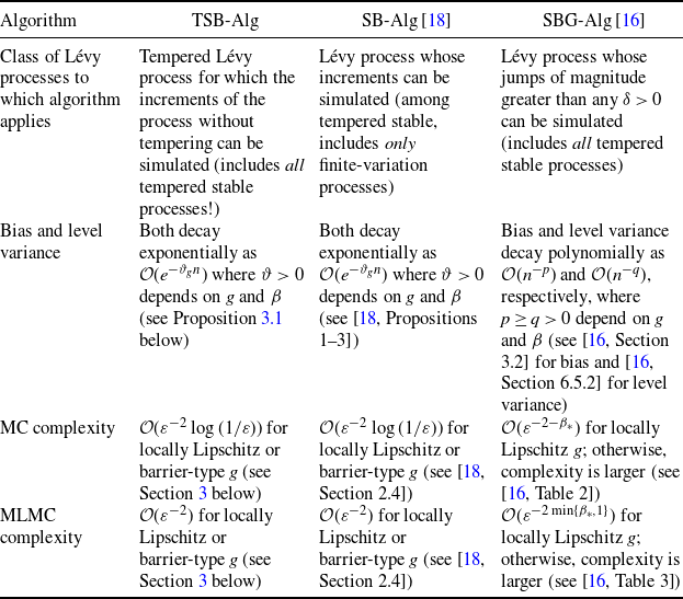
Exact simulation of the drawdown is currently out of reach. Under the assumption that the increments of the Lévy process X can be simulated (an assumption not satisfied by tempered stable models of infinite variation), the algorithm SB-Alg in [Reference González Cázares, Mijatović and Uribe Bravo18] has a geometrically small bias, significantly outperforming other algorithms for which the computational complexity analysis has been carried out. For instance, the computational complexity analysis for the procedures presented in [Reference Figueroa-López and Tankov12, Reference Kim and Kim24], applicable to tempered stable processes of finite variation, has not been carried out, so that a direct quantitative comparison with SB-Alg [Reference González Cázares, Mijatović and Uribe Bravo18] is not possible at present. If the increments cannot be sampled, a general approach utilises the Gaussian approximation of small jumps, in which case the algorithm SBG-Alg [Reference González Cázares and Mijatović16] outperforms its competitors (e.g. random walk approximation; see [Reference González Cázares and Mijatović16] for details), while retaining polynomially small bias. Thus it suffices to compare TSB-Alg below with SB-Alg [Reference González Cázares, Mijatović and Uribe Bravo18] and SBG-Alg [Reference González Cázares and Mijatović16]. Table 1 below provides a summary of the properties of TSB-Alg, SB-Alg, and SBG-Alg as well as the asymptotic computational complexities of the corresponding MC and MLMC estimators based on these algorithms (see also Subsection 3.4 below for a detailed comparison).
The stick-breaking (SB) representation in (2) plays a central role in the algorithms TSB-Alg, SB-Alg, and SBG-Alg. The SB representation was used in [Reference González Cázares, Mijatović and Uribe Bravo18] to obtain an approximation
 $\chi_n$
of
$\chi_n$
of
 $\chi\,:\!=\,(X_T,\overline{X}_T,\tau_T(X))$
that converges geometrically fast in the computational cost when the increments of X can be simulated exactly. In [Reference González Cázares and Mijatović16], the same representation was used in conjunction with a small-jump Gaussian approximation for arbitrary Lévy processes. In the present work we address a situation in between those of the two aforementioned papers, using TSB-Alg below. TSB-Alg preserves the geometric convergence in the computational cost of SB-Alg, while being applicable to general tempered stable processes (unlike SB-Alg [Reference González Cázares, Mijatović and Uribe Bravo18] in the infinite-variation case) and asymptotically outperforming SBG-Alg [Reference González Cázares and Mijatović16]; see Table 1 for an overview.
$\chi\,:\!=\,(X_T,\overline{X}_T,\tau_T(X))$
that converges geometrically fast in the computational cost when the increments of X can be simulated exactly. In [Reference González Cázares and Mijatović16], the same representation was used in conjunction with a small-jump Gaussian approximation for arbitrary Lévy processes. In the present work we address a situation in between those of the two aforementioned papers, using TSB-Alg below. TSB-Alg preserves the geometric convergence in the computational cost of SB-Alg, while being applicable to general tempered stable processes (unlike SB-Alg [Reference González Cázares, Mijatović and Uribe Bravo18] in the infinite-variation case) and asymptotically outperforming SBG-Alg [Reference González Cázares and Mijatović16]; see Table 1 for an overview.
Table 1. Summary of the properties of TSB-Alg, SB-Alg [Reference González Cázares, Mijatović and Uribe Bravo18], and SBG-Alg [Reference González Cázares and Mijatović16]. The index
 $\beta_*$
, defined in (21) below, is slightly larger than the Blumenthal–Getoor index
$\beta_*$
, defined in (21) below, is slightly larger than the Blumenthal–Getoor index
 $\beta$
; see Section 5 below for details. The bias and level variance are parametrised by computational effort n as
$\beta$
; see Section 5 below for details. The bias and level variance are parametrised by computational effort n as
 $n\to\infty$
, while the MC and MLMC complexities are parametrised by the accuracy
$n\to\infty$
, while the MC and MLMC complexities are parametrised by the accuracy
 $\varepsilon$
(i.e., the mean squared error is at most
$\varepsilon$
(i.e., the mean squared error is at most
 $\varepsilon^2$
) as
$\varepsilon^2$
) as
 $\varepsilon\to 0$
.
$\varepsilon\to 0$
.
1.3. Organisation
The remainder of the paper is structured as follows. In Section 2 we recall the SB representation and construct TSB-Alg. In Section 3 we describe the geometric decay of the bias and the strong error in
 $L^p$
and explain what the computational complexities of the MC and MLMC estimators are. We discuss briefly in Subsection 3.3 the construction and properties of unbiased estimators based on TSB-Alg. In Subsection 3.4 we provide an in-depth comparison of TSB-Alg with the SB and SBG algorithms, identifying where each algorithm outperforms the others. In Section 4 we consider the case of tempered stable processes and illustrate the previously described results with numerical examples. The proofs of all the results except Theorem 2.1, which is stated and proved in Section 2, are given in Section 5 below.
$L^p$
and explain what the computational complexities of the MC and MLMC estimators are. We discuss briefly in Subsection 3.3 the construction and properties of unbiased estimators based on TSB-Alg. In Subsection 3.4 we provide an in-depth comparison of TSB-Alg with the SB and SBG algorithms, identifying where each algorithm outperforms the others. In Section 4 we consider the case of tempered stable processes and illustrate the previously described results with numerical examples. The proofs of all the results except Theorem 2.1, which is stated and proved in Section 2, are given in Section 5 below.
2. The tempered stick-breaking algorithm
Let
 $T>0$
be a time horizon and
$T>0$
be a time horizon and
 ${\boldsymbol\lambda}=(\lambda_+,\lambda_-)\in\mathbb{R}_+^2$
a vector with non-negative coordinates, different from the origin
${\boldsymbol\lambda}=(\lambda_+,\lambda_-)\in\mathbb{R}_+^2$
a vector with non-negative coordinates, different from the origin
 ${\boldsymbol0}=(0,0)$
. A stochastic process
${\boldsymbol0}=(0,0)$
. A stochastic process
 $X=(X_t)_{t\in[0,T]}$
is said to be a tempered Lévy process under the probability measure
$X=(X_t)_{t\in[0,T]}$
is said to be a tempered Lévy process under the probability measure
 $\mathbb{P}_{\boldsymbol\lambda}$
if its characteristic function satisfies
$\mathbb{P}_{\boldsymbol\lambda}$
if its characteristic function satisfies
 \begin{align} t^{-1}\log\mathbb{E}_{\boldsymbol\lambda}\big[e^{iuX_t}\big]= & iub_{\boldsymbol\lambda}-\frac{1}{2}\sigma^2u^2+\int_{\mathbb{R}\setminus\{0\}}\big(e^{iux}-1-iux\cdot\mathbb{1}_{({-}1,1)}(x)\big)\nu_{\boldsymbol\lambda}(\textrm{d} x),\\&\qquad\qquad\qquad\qquad\qquad\qquad\qquad \text{for all }u\in\mathbb{R},\,t>0,\end{align}
where
 $\mathbb{E}_{\boldsymbol\lambda}$
denotes the expectation under the probability measure
$\mathbb{E}_{\boldsymbol\lambda}$
denotes the expectation under the probability measure
 $\mathbb{P}_{\boldsymbol\lambda}$
, and the generating (or Lévy) triplet
$\mathbb{P}_{\boldsymbol\lambda}$
, and the generating (or Lévy) triplet
 $(\sigma^2,\nu_{\boldsymbol\lambda},b_{\boldsymbol\lambda})$
is given by
$(\sigma^2,\nu_{\boldsymbol\lambda},b_{\boldsymbol\lambda})$
is given by
 \begin{equation}\nu_{\boldsymbol\lambda}(\textrm{d} x) \,:\!=\, e^{-\lambda_{{\textrm{sgn}}(x)}|x|}\nu(\textrm{d} x)\qquad \text{and}\qquad b_{\boldsymbol\lambda} \,:\!=\, b + \int_{({-}1,1)}x\big(e^{-\lambda_{{\textrm{sgn}}(x)}|x|}-1\big)\nu(\textrm{d} x),\end{equation}
where
 $\sigma^2\in\mathbb{R}_+$
,
$\sigma^2\in\mathbb{R}_+$
,
 $b\in\mathbb{R}$
, and
$b\in\mathbb{R}$
, and
 $\nu$
is a Lévy measure on
$\nu$
is a Lévy measure on
 $\mathbb{R}\setminus\{0\}$
, i.e.
$\mathbb{R}\setminus\{0\}$
, i.e.
 $\nu$
satisfies
$\nu$
satisfies
 $\int_{(-1,1)}x^2\nu(\textrm{d} x)<\infty$
and
$\int_{(-1,1)}x^2\nu(\textrm{d} x)<\infty$
and
 $\nu(\mathbb{R}\setminus({-}1,1))<\infty$
. (All Lévy triplets in this paper are given with respect to the cutoff function
$\nu(\mathbb{R}\setminus({-}1,1))<\infty$
. (All Lévy triplets in this paper are given with respect to the cutoff function
 $x\mapsto\mathbb{1}_{(-1,1)}(x)$
, and the sign function in (1) is defined as
$x\mapsto\mathbb{1}_{(-1,1)}(x)$
, and the sign function in (1) is defined as
 ${\textrm{sgn}}(x)\,:\!=\,\mathbb{1}_{\{x>0\}}-\mathbb{1}_{\{x<0\}}$
.) The triplet
${\textrm{sgn}}(x)\,:\!=\,\mathbb{1}_{\{x>0\}}-\mathbb{1}_{\{x<0\}}$
.) The triplet
 $\big(\sigma^2,\nu_{\boldsymbol\lambda},b_{\boldsymbol\lambda}\big)$
uniquely determines the law of X via the Lévy–Khintchine formula for the characteristic function of
$\big(\sigma^2,\nu_{\boldsymbol\lambda},b_{\boldsymbol\lambda}\big)$
uniquely determines the law of X via the Lévy–Khintchine formula for the characteristic function of
 $X_t$
for
$X_t$
for
 $t>0$
given in the displays above (for details, see [Reference Sato35, Theorems 7.10 and 8.1, Definition 8.2]).
$t>0$
given in the displays above (for details, see [Reference Sato35, Theorems 7.10 and 8.1, Definition 8.2]).
Our aim is to sample from the law of the statistic
 $(X_T,\overline{X}_T,\tau_T)$
consisting of the position
$(X_T,\overline{X}_T,\tau_T)$
consisting of the position
 $X_T$
of the process X at T, the supremum
$X_T$
of the process X at T, the supremum
 $\overline{X}_T\,:\!=\,\sup\{X_s:s\in[0,T]\}$
of X on the time interval [0,T], and the time
$\overline{X}_T\,:\!=\,\sup\{X_s:s\in[0,T]\}$
of X on the time interval [0,T], and the time
 $\tau_T\,:\!=\,\inf\{s\in[0,T]:\overline{X}_s=\overline{X}_T\}$
at which the supremum was attained in [0,T]. By [Reference González Cázares, Mijatović and Uribe Bravo18, Theorem 1] there exists a coupling
$\tau_T\,:\!=\,\inf\{s\in[0,T]:\overline{X}_s=\overline{X}_T\}$
at which the supremum was attained in [0,T]. By [Reference González Cázares, Mijatović and Uribe Bravo18, Theorem 1] there exists a coupling
 $(X,Y,\ell)$
under a probability measure
$(X,Y,\ell)$
under a probability measure
 $\mathbb{P}_{\boldsymbol\lambda}$
, such that
$\mathbb{P}_{\boldsymbol\lambda}$
, such that
 $\ell=(\ell_n)_{n\in\mathbb{N}}$
is a stick-breaking process on [0,T] based on the uniform law
$\ell=(\ell_n)_{n\in\mathbb{N}}$
is a stick-breaking process on [0,T] based on the uniform law
 $\textrm{U}(0,1)$
(i.e.
$\textrm{U}(0,1)$
(i.e.
 $L_0\,:\!=\,T$
,
$L_0\,:\!=\,T$
,
 $L_n\,:\!=\,L_{n-1}U_n$
, and
$L_n\,:\!=\,L_{n-1}U_n$
, and
 $\ell_n\,:\!=\,L_{n-1}-L_n$
for
$\ell_n\,:\!=\,L_{n-1}-L_n$
for
 $n\in\mathbb{N}$
, where the
$n\in\mathbb{N}$
, where the
 $U_n$
are independent and identically distributed (i.i.d.) as
$U_n$
are independent and identically distributed (i.i.d.) as
 $\textrm{U}(0,1)$
), independent of the Lévy process Y with law equal to that of X, and the SB representation holds
$\textrm{U}(0,1)$
), independent of the Lévy process Y with law equal to that of X, and the SB representation holds
 $\mathbb{P}_{\boldsymbol\lambda}$
-almost surely (a.s.):
$\mathbb{P}_{\boldsymbol\lambda}$
-almost surely (a.s.):
 \begin{equation}\chi \,:\!=\, (X_T,\overline{X}_T,\tau_T)=\sum_{n=1}^\infty \big(\xi_n,\max\{\xi_n,0\},\ell_n\cdot\mathbb{1}_{\{\xi_n>0\}}\big),\quad \text{where}\quad \xi_n \,:\!=\, Y_{L_{n-1}}-Y_{L_n}, n\in\mathbb{N}.\end{equation}
We stress that
 $\ell$
is not independent of X. In fact
$\ell$
is not independent of X. In fact
 $(\ell,Y)$
can be expressed naturally through the geometry of the path of X (see [Reference Pitman and Uribe Bravo32, Theorem 1] and the coupling in [Reference González Cázares, Mijatović and Uribe Bravo18]), but further details of the coupling are not important for our purposes. The key step in the construction of our algorithm is given by the following theorem. Its proof is based on the coupling described above and the change-of-measure theorem for Lévy processes [Reference Sato35, Theorems 33.1 and 33.2].
$(\ell,Y)$
can be expressed naturally through the geometry of the path of X (see [Reference Pitman and Uribe Bravo32, Theorem 1] and the coupling in [Reference González Cázares, Mijatović and Uribe Bravo18]), but further details of the coupling are not important for our purposes. The key step in the construction of our algorithm is given by the following theorem. Its proof is based on the coupling described above and the change-of-measure theorem for Lévy processes [Reference Sato35, Theorems 33.1 and 33.2].
Theorem 2.1.
Denote by
 $\sigma B$
,
$\sigma B$
,
 $Y^{{(+)}}$
,
$Y^{{(+)}}$
,
 $Y^{{(-)}}$
the independent Lévy processes with generating triplets
$Y^{{(-)}}$
the independent Lévy processes with generating triplets
 $\big(\sigma^2,0,0\big)$
,
$\big(\sigma^2,0,0\big)$
,
 $(0,\nu_{\boldsymbol\lambda}|_{(0,\infty)},0)$
,
$(0,\nu_{\boldsymbol\lambda}|_{(0,\infty)},0)$
,
 $(0,\nu_{\boldsymbol\lambda}|_{(-\infty,0)},0)$
, respectively, satisfying
$(0,\nu_{\boldsymbol\lambda}|_{(-\infty,0)},0)$
, respectively, satisfying
 $Y_t=\sigma B_t+Y_t^{{(+)}}+Y_t^{{(-)}}+b_{\boldsymbol\lambda} t$
for all
$Y_t=\sigma B_t+Y_t^{{(+)}}+Y_t^{{(-)}}+b_{\boldsymbol\lambda} t$
for all
 $t\in[0,T]$
,
$t\in[0,T]$
,
 $\mathbb{P}_{\boldsymbol\lambda}$
-a.s. Let
$\mathbb{P}_{\boldsymbol\lambda}$
-a.s. Let
 $\mathbb{E}_{\boldsymbol\lambda}$
(resp.
$\mathbb{E}_{\boldsymbol\lambda}$
(resp.
 $\mathbb{E}_{\boldsymbol0}$
) be the expectation under
$\mathbb{E}_{\boldsymbol0}$
) be the expectation under
 $\mathbb{P}_{\boldsymbol\lambda}$
(resp.
$\mathbb{P}_{\boldsymbol\lambda}$
(resp.
 $\mathbb{P}_{\boldsymbol0}$
) and define
$\mathbb{P}_{\boldsymbol0}$
) and define
 \begin{align}\Upsilon_{\boldsymbol\lambda}&\,:\!=\, \exp\big({-}\lambda_+Y^{{(+)}}_T +\lambda_-Y^{{(-)}}_T - \mu_{\boldsymbol\lambda} T\big), \qquad \text{where}\end{align}
 \begin{align}\mu_{\boldsymbol\lambda}&\,:\!=\, \int_\mathbb{R}\big(e^{-\lambda_{{\textrm{sgn}}(x)}|x|}-1 +\lambda_{{\textrm{sgn}}(x)}|x|\cdot\mathbb{1}_{({-}1,1)}(x)\big)\nu(\textrm{d} x).\end{align}
Then for any
 $\sigma(\ell,\xi)$
-measurable random variable
$\sigma(\ell,\xi)$
-measurable random variable
 $\zeta$
with
$\zeta$
with
 $\mathbb{E}_{\boldsymbol\lambda}|\zeta|<\infty$
we have
$\mathbb{E}_{\boldsymbol\lambda}|\zeta|<\infty$
we have
 $\mathbb{E}_{\boldsymbol\lambda}[\zeta]= \mathbb{E}_{\boldsymbol0}[\zeta\Upsilon_{\boldsymbol\lambda}]$
.
$\mathbb{E}_{\boldsymbol\lambda}[\zeta]= \mathbb{E}_{\boldsymbol0}[\zeta\Upsilon_{\boldsymbol\lambda}]$
.
Proof. The exponential change-of-measure theorem for Lévy processes (see [Reference Sato35, Theorems 33.1 and 33.2]) implies that for any measurable function F with
 $\mathbb{E}_{\boldsymbol\lambda} |F((Y_t)_{t\in[0,T]})|<\infty$
, we have the identity
$\mathbb{E}_{\boldsymbol\lambda} |F((Y_t)_{t\in[0,T]})|<\infty$
, we have the identity
 $\mathbb{E}_{\boldsymbol\lambda}[F((Y_t)_{t\in[0,T]})]=\mathbb{E}_{\boldsymbol0}[F((Y_t)_{t\in[0,T]})\Upsilon_{\boldsymbol\lambda}]$
, where
$\mathbb{E}_{\boldsymbol\lambda}[F((Y_t)_{t\in[0,T]})]=\mathbb{E}_{\boldsymbol0}[F((Y_t)_{t\in[0,T]})\Upsilon_{\boldsymbol\lambda}]$
, where
 $\Upsilon_{\boldsymbol\lambda}$
is defined in (3) in the statement of Theorem 2.1. Since the stick-breaking process
$\Upsilon_{\boldsymbol\lambda}$
is defined in (3) in the statement of Theorem 2.1. Since the stick-breaking process
 $\ell$
is independent of Y under both
$\ell$
is independent of Y under both
 $\mathbb{P}_{\boldsymbol\lambda}$
and
$\mathbb{P}_{\boldsymbol\lambda}$
and
 $\mathbb{P}_{\boldsymbol0}$
, this property extends to measurable functions of
$\mathbb{P}_{\boldsymbol0}$
, this property extends to measurable functions of
 $(\ell, (Y_t)_{t\in[0,T]})$
and thus to measurable functions of
$(\ell, (Y_t)_{t\in[0,T]})$
and thus to measurable functions of
 $(\ell,\xi)$
, as claimed.
$(\ell,\xi)$
, as claimed.
By the equality in (2), the measurable function
 $\zeta$
of the sequences
$\zeta$
of the sequences
 $\ell$
and
$\ell$
and
 $\xi$
in Theorem 2.1 may be equal either to
$\xi$
in Theorem 2.1 may be equal either to
 $g(\chi)$
(for any integrable function g of the statistic
$g(\chi)$
(for any integrable function g of the statistic
 $\chi$
) or to its approximation
$\chi$
) or to its approximation
 $g(\chi_n)$
, where
$g(\chi_n)$
, where
 $\chi_n$
is as introduced in [Reference González Cázares, Mijatović and Uribe Bravo18]:
$\chi_n$
is as introduced in [Reference González Cázares, Mijatović and Uribe Bravo18]:
 \begin{equation}\begin{split}\chi_n&\,:\!=\,\big(Y_{L_n},\max\{Y_{L_n},0\},L_n\cdot\mathbb{1}_{\{Y_{L_n}>0\}}\big) +\sum_{k=1}^n\big(\xi_k,\max\{\xi_k,0\},\ell_k\cdot\mathbb{1}_{\{\xi_k>0\}}\big).\end{split}\end{equation}
Theorem 2.1 enables us to sample
 $\chi_n$
under the probability measure
$\chi_n$
under the probability measure
 $\mathbb{P}_{\boldsymbol0}$
, which for any tempered stable process X makes the increments of Y stable and thus easy to simulate. Under
$\mathbb{P}_{\boldsymbol0}$
, which for any tempered stable process X makes the increments of Y stable and thus easy to simulate. Under
 $\mathbb{P}_{\boldsymbol0}$
, the law of
$\mathbb{P}_{\boldsymbol0}$
, the law of
 $Y_t$
equals that of
$Y_t$
equals that of
 $Y_t^{{(+)}}+Y_t^{{(-)}}+\sigma B_t+b t$
, where
$Y_t^{{(+)}}+Y_t^{{(-)}}+\sigma B_t+b t$
, where
 $\sigma B_t+b t$
is normal
$\sigma B_t+b t$
is normal
 $N\big(bt,\sigma^2 t\big)$
with mean bt and variance
$N\big(bt,\sigma^2 t\big)$
with mean bt and variance
 $\sigma^2 t$
and the Lévy processes
$\sigma^2 t$
and the Lévy processes
 $Y^{{(+)}}$
and
$Y^{{(+)}}$
and
 $Y^{{(-)}}$
have triplets
$Y^{{(-)}}$
have triplets
 $(0,\nu|_{(0,\infty)},0)$
and
$(0,\nu|_{(0,\infty)},0)$
and
 $(0,\nu|_{(-\infty,0)},0)$
, respectively. Denote their distribution functions by
$(0,\nu|_{(-\infty,0)},0)$
, respectively. Denote their distribution functions by
 $F^{{(\pm)}}(t,x)\,:\!=\,\mathbb{P}_{\boldsymbol0}\big(Y_t^{{(\pm)}}\le x\big)$
,
$F^{{(\pm)}}(t,x)\,:\!=\,\mathbb{P}_{\boldsymbol0}\big(Y_t^{{(\pm)}}\le x\big)$
,
 $x\in\mathbb{R}$
,
$x\in\mathbb{R}$
,
 $t>0$
.
$t>0$
.
TSB-Alg

Note that the output
 $g(\chi_n)\Upsilon_{\boldsymbol\lambda}$
of TSB-Alg is sampled under
$g(\chi_n)\Upsilon_{\boldsymbol\lambda}$
of TSB-Alg is sampled under
 $\mathbb{P}_{\boldsymbol0}$
and, by Theorem 2.1 above, is unbiased since
$\mathbb{P}_{\boldsymbol0}$
and, by Theorem 2.1 above, is unbiased since
 $\mathbb{E}_{\boldsymbol0}[g(\chi_n)\Upsilon_{\boldsymbol\lambda}]=\mathbb{E}_{\boldsymbol\lambda}[g(\chi_n)]$
. As our aim is to obtain MC and MLMC estimators for
$\mathbb{E}_{\boldsymbol0}[g(\chi_n)\Upsilon_{\boldsymbol\lambda}]=\mathbb{E}_{\boldsymbol\lambda}[g(\chi_n)]$
. As our aim is to obtain MC and MLMC estimators for
 $\mathbb{E}_{\boldsymbol\lambda}[g(\chi)]$
, our next task is to understand the expected error of TSB-Alg; see (6) in Subsection 3.1 below. In [Reference González Cázares, Mijatović and Uribe Bravo18] it was proved that the approximation
$\mathbb{E}_{\boldsymbol\lambda}[g(\chi)]$
, our next task is to understand the expected error of TSB-Alg; see (6) in Subsection 3.1 below. In [Reference González Cázares, Mijatović and Uribe Bravo18] it was proved that the approximation
 $\chi_n$
converges geometrically fast in computational effort (or equivalently as
$\chi_n$
converges geometrically fast in computational effort (or equivalently as
 $n\to\infty$
) to
$n\to\infty$
) to
 $\chi$
if the increments of Y can be sampled under
$\chi$
if the increments of Y can be sampled under
 $\mathbb{P}_{\boldsymbol\lambda}$
(see [Reference González Cázares, Mijatović and Uribe Bravo18] for more details and a discussion of the benefits of the ‘correction term’
$\mathbb{P}_{\boldsymbol\lambda}$
(see [Reference González Cázares, Mijatović and Uribe Bravo18] for more details and a discussion of the benefits of the ‘correction term’
 $(Y_{L_n},\max\{Y_{L_n},0\},L_n\cdot\mathbb{1}_{\{Y_{L_n}>0\}})$
in (5)). Theorem 2.1 allows us to weaken this requirement in the context of tempered Lévy processes, by requiring that we be able to sample the increments of Y under
$(Y_{L_n},\max\{Y_{L_n},0\},L_n\cdot\mathbb{1}_{\{Y_{L_n}>0\}})$
in (5)). Theorem 2.1 allows us to weaken this requirement in the context of tempered Lévy processes, by requiring that we be able to sample the increments of Y under
 $\mathbb{P}_{\boldsymbol0}$
. The main application of TSB-Alg is to general tempered stable processes, as the simulation of their increments is currently out of reach for many cases of interest (see Section 3.4 below for comparison with existing methods when it is not), making the main algorithm in [Reference González Cázares, Mijatović and Uribe Bravo18] not applicable. Moreover, Theorem 2.1 allows us to retain the geometric convergence of
$\mathbb{P}_{\boldsymbol0}$
. The main application of TSB-Alg is to general tempered stable processes, as the simulation of their increments is currently out of reach for many cases of interest (see Section 3.4 below for comparison with existing methods when it is not), making the main algorithm in [Reference González Cázares, Mijatović and Uribe Bravo18] not applicable. Moreover, Theorem 2.1 allows us to retain the geometric convergence of
 $\chi_n$
established in [Reference González Cázares, Mijatović and Uribe Bravo18]; see Section 3 below for details.
$\chi_n$
established in [Reference González Cázares, Mijatović and Uribe Bravo18]; see Section 3 below for details.
3. Monte Carlo and multilevel Monte Carlo estimators based on TSB-Alg
3.1. Bias of TSB-Alg
An application of Theorem 2.1 implies that the bias of TSB-Alg equals
 \begin{equation}\mathbb{E}_{\boldsymbol\lambda}[g(\chi)]-\mathbb{E}_{\boldsymbol0}[g(\chi_n)\Upsilon_{\boldsymbol\lambda}]=\mathbb{E}_{\boldsymbol0}\big[\Delta_n^g\big], \quad \text{where $\Delta_n^g\,:\!=\,(g(\chi)-g(\chi_n))\Upsilon_{\boldsymbol\lambda}$}.\end{equation}
The natural coupling
 $\big(\chi,\chi_n, Y_T^{{(+)}}, Y_T^{{(-)}}\big)$
in (6) is defined by
$\big(\chi,\chi_n, Y_T^{{(+)}}, Y_T^{{(-)}}\big)$
in (6) is defined by
 $Y_T^{{(\pm)}}\,:\!=\,\sum_{k=1}^{\infty}\xi_k^{{(\pm)}}$
,
$Y_T^{{(\pm)}}\,:\!=\,\sum_{k=1}^{\infty}\xi_k^{{(\pm)}}$
,
 $\xi_k\,:\!=\,\xi_k^{{(+)}}+\xi_k^{{(-)}}+ \eta_k$
for all
$\xi_k\,:\!=\,\xi_k^{{(+)}}+\xi_k^{{(-)}}+ \eta_k$
for all
 $k\in\mathbb{N}$
,
$k\in\mathbb{N}$
,
 $\chi$
in (2), and
$\chi$
in (2), and
 $\chi_n$
in (5) with
$\chi_n$
in (5) with
 $Y_{L_n}\,:\!=\,\sum_{k=n+1}^\infty \xi_k$
, where, conditional on the stick-breaking process
$Y_{L_n}\,:\!=\,\sum_{k=n+1}^\infty \xi_k$
, where, conditional on the stick-breaking process
 $\ell=(\ell_k)_{k\in\mathbb{N}}$
, the random variables
$\ell=(\ell_k)_{k\in\mathbb{N}}$
, the random variables
 $\{\xi_k^{{(\pm)}},\eta_k:k\in\mathbb{N}\}$
are independent and distributed as
$\{\xi_k^{{(\pm)}},\eta_k:k\in\mathbb{N}\}$
are independent and distributed as
 $\xi_k^{{(\pm)}}\sim F^{{(\pm)}}(\ell_k,\cdot)$
and
$\xi_k^{{(\pm)}}\sim F^{{(\pm)}}(\ell_k,\cdot)$
and
 $\eta_k\sim N\big(\ell_k b,\sigma^2 \ell_k\big)$
for
$\eta_k\sim N\big(\ell_k b,\sigma^2 \ell_k\big)$
for
 $k\in\mathbb{N}$
.
$k\in\mathbb{N}$
.
The following result presents the decay of the strong error
 $\Delta_n^g$
for Lipschitz, locally Lipschitz, and two classes of barrier-type discontinuous payoffs that arise frequently in applications. Observe that, in all cases and under the corresponding mild assumptions, the pth moment of the strong error
$\Delta_n^g$
for Lipschitz, locally Lipschitz, and two classes of barrier-type discontinuous payoffs that arise frequently in applications. Observe that, in all cases and under the corresponding mild assumptions, the pth moment of the strong error
 $\Delta_n^g$
decays exponentially fast in n with a rate
$\Delta_n^g$
decays exponentially fast in n with a rate
 $\vartheta>0$
that depends on the payoff g, the index
$\vartheta>0$
that depends on the payoff g, the index
 $\beta_*$
defined in (21) below, and the degree p of the considered moment. In Proposition 3.1 and throughout the paper, the notation
$\beta_*$
defined in (21) below, and the degree p of the considered moment. In Proposition 3.1 and throughout the paper, the notation
 $f(n)=\mathcal{O}(g(n))$
as
$f(n)=\mathcal{O}(g(n))$
as
 $n\to\infty$
for functions
$n\to\infty$
for functions
 $f,g:\mathbb{N}\to(0,\infty)$
means
$f,g:\mathbb{N}\to(0,\infty)$
means
 $\limsup_{n\to\infty}f(n)/g(n)<\infty$
. Put differently,
$\limsup_{n\to\infty}f(n)/g(n)<\infty$
. Put differently,
 $f(n)=\mathcal{O}(g(n))$
is equivalent to f(n) being bounded above by
$f(n)=\mathcal{O}(g(n))$
is equivalent to f(n) being bounded above by
 $C_0 g(n)$
for some constant
$C_0 g(n)$
for some constant
 $C_0>0$
and all
$C_0>0$
and all
 $n\in\mathbb{N}$
.
$n\in\mathbb{N}$
.
Proposition 3.1.
Let
 ${\boldsymbol\lambda}=(\lambda_+,\lambda_-)$
,
${\boldsymbol\lambda}=(\lambda_+,\lambda_-)$
,
 $\nu$
, and
$\nu$
, and
 $\sigma^2$
be as in Section 2, and fix
$\sigma^2$
be as in Section 2, and fix
 $p\ge 1$
. Then, for the classes of payoffs
$p\ge 1$
. Then, for the classes of payoffs
 $g(\chi)=g(X_T,\overline{X}_T, \tau_T)$
below, the strong error of TSB-Alg decays as follows (as
$g(\chi)=g(X_T,\overline{X}_T, \tau_T)$
below, the strong error of TSB-Alg decays as follows (as
 $n\to\infty$
).
$n\to\infty$
).
(Lipschitz.) Suppose
 $|g(x,y,t)-g(x,y',t')|\le K(|y-y'|+|t-t'|)$
for some K and all
$|g(x,y,t)-g(x,y',t')|\le K(|y-y'|+|t-t'|)$
for some K and all
 $(x,y,y',t,t')\in\mathbb{R}\times\mathbb{R}_+^2\times[0,T]^2$
. Then
$(x,y,y',t,t')\in\mathbb{R}\times\mathbb{R}_+^2\times[0,T]^2$
. Then
 $\mathbb{E}_{{\boldsymbol0}}\big[\big|\Delta_n^g\big|^p\big]=\mathcal{O}\big(e^{-\vartheta_p n}\big)$
, where
$\mathbb{E}_{{\boldsymbol0}}\big[\big|\Delta_n^g\big|^p\big]=\mathcal{O}\big(e^{-\vartheta_p n}\big)$
, where
 $\vartheta_p\in[\log(3/2),\log2]$
is in (23) below.
$\vartheta_p\in[\log(3/2),\log2]$
is in (23) below.
(Locally Lipschitz.) Let
 $|g(x,y,t)-g(x,y',t')|\le K(|y-y'|+|t-t'|)e^{\max\{y,y'\}}$
for some constant
$|g(x,y,t)-g(x,y',t')|\le K(|y-y'|+|t-t'|)e^{\max\{y,y'\}}$
for some constant
 $K>0$
and all
$K>0$
and all
 $(x,y,y',t,t')\in\mathbb{R}\times\mathbb{R}_+^2\times[0,T]^2$
. If
$(x,y,y',t,t')\in\mathbb{R}\times\mathbb{R}_+^2\times[0,T]^2$
. If
 $\lambda_+\geq q > 1$
and
$\lambda_+\geq q > 1$
and
 $\int_{[1,\infty)}e^{p(q-\lambda_+)x}\nu(\textrm{d} x)<\infty$
, then
$\int_{[1,\infty)}e^{p(q-\lambda_+)x}\nu(\textrm{d} x)<\infty$
, then
 $\mathbb{E}_{{\boldsymbol0}}\big[\big|\Delta_n^g\big|^p\big]=\mathcal{O}\big(e^{-( \vartheta_{pr}/r)n}\big)$
, where
$\mathbb{E}_{{\boldsymbol0}}\big[\big|\Delta_n^g\big|^p\big]=\mathcal{O}\big(e^{-( \vartheta_{pr}/r)n}\big)$
, where
 $r\,:\!=\,(1-1/q)^{-1}>1$
and
$r\,:\!=\,(1-1/q)^{-1}>1$
and
 $\vartheta_{pr}\in[\log(3/2),\log2]$
is as in (23).
$\vartheta_{pr}\in[\log(3/2),\log2]$
is as in (23).
(Barrier type 1.) Suppose
 $g(\chi)=h(X_T)\cdot\mathbb{1}\{\overline{X}_T\le M\}$
for some
$g(\chi)=h(X_T)\cdot\mathbb{1}\{\overline{X}_T\le M\}$
for some
 $M>0$
and a measurable bounded function
$M>0$
and a measurable bounded function
 $h:\mathbb{R}\to\mathbb{R}$
. If
$h:\mathbb{R}\to\mathbb{R}$
. If
 $\mathbb{P}_{{\boldsymbol0}}(M<\overline{X}_T\le M+x)\le Kx$
for some
$\mathbb{P}_{{\boldsymbol0}}(M<\overline{X}_T\le M+x)\le Kx$
for some
 $K>0$
and all
$K>0$
and all
 $x\ge0$
, then for
$x\ge0$
, then for
 $\alpha_*\in (1,2]$
in (22) and any
$\alpha_*\in (1,2]$
in (22) and any
 $\gamma\in(0,1)$
we have
$\gamma\in(0,1)$
we have
 $\mathbb{E}_{{\boldsymbol0}}\big[\big|\Delta_n^g\big|^p\big]=\mathcal{O}\big(e^{-[\gamma\log(2)/(\gamma+\alpha_*)]n}\big)$
. Moreover, we may take
$\mathbb{E}_{{\boldsymbol0}}\big[\big|\Delta_n^g\big|^p\big]=\mathcal{O}\big(e^{-[\gamma\log(2)/(\gamma+\alpha_*)]n}\big)$
. Moreover, we may take
 $\gamma=1$
if any of the following hold:
$\gamma=1$
if any of the following hold:
 $\sigma^2>0$
or
$\sigma^2>0$
or
 $\int_{(-1,1)}|x|\nu(\textrm{d} x)<\infty$
or Assumption 5.1 below.
$\int_{(-1,1)}|x|\nu(\textrm{d} x)<\infty$
or Assumption 5.1 below.
(Barrier type 2.) Suppose
 $g(\chi)=h(X_T,\overline{X}_T)\cdot\mathbb{1}\{\tau_T\le s\}$
, where
$g(\chi)=h(X_T,\overline{X}_T)\cdot\mathbb{1}\{\tau_T\le s\}$
, where
 $s\in(0,T)$
, and h is measurable and bounded with
$s\in(0,T)$
, and h is measurable and bounded with
 $|h(x,y)-h(x,y')|\le K|y-y'|$
for some
$|h(x,y)-h(x,y')|\le K|y-y'|$
for some
 $K>0$
and all
$K>0$
and all
 $(x,y,y')\in\mathbb{R}\times\mathbb{R}_+^2$
. If
$(x,y,y')\in\mathbb{R}\times\mathbb{R}_+^2$
. If
 $\sigma^2>0$
or
$\sigma^2>0$
or
 $\nu(\mathbb{R}\setminus\{0\})=\infty$
, then
$\nu(\mathbb{R}\setminus\{0\})=\infty$
, then
 $\mathbb{E}_{{\boldsymbol0}}\big[\big|\Delta_n^g\big|^p\big]=\mathcal{O}\big(e^{-n/e}\big)$
.
$\mathbb{E}_{{\boldsymbol0}}\big[\big|\Delta_n^g\big|^p\big]=\mathcal{O}\big(e^{-n/e}\big)$
.
Remark 3.1. (i) The proof of Proposition 3.1, given in Section 5 below, is based on Theorem 2.1 and analogous bounds in [Reference González Cázares, Mijatović and Uribe Bravo18] (for Lipschitz, locally Lipschitz, and barrier-type-1 payoffs) and [Reference González Cázares and Mijatović16] (for barrier-type-2 payoffs). In particular, in the proof of Proposition 3.1 below, we need not assume
 $\lambda_+>0$
to apply [Reference González Cázares, Mijatović and Uribe Bravo18, Proposition 1], which works under our standing assumption
$\lambda_+>0$
to apply [Reference González Cázares, Mijatović and Uribe Bravo18, Proposition 1], which works under our standing assumption
 ${\boldsymbol\lambda}\neq {\boldsymbol0}$
.
${\boldsymbol\lambda}\neq {\boldsymbol0}$
.
(ii) For barrier option payoffs under a tempered stable process X (i.e. the barrier-type-1 class in Proposition 3.1), we may take
 $\gamma=1$
since X satisfies either
$\gamma=1$
since X satisfies either
 $\int_{(-1,1)}|x|\nu(\textrm{d} x)<\infty$
or Assumption 5.1.
$\int_{(-1,1)}|x|\nu(\textrm{d} x)<\infty$
or Assumption 5.1.
(iii) The restriction
 $p\ge 1$
is not essential, as we may consider any
$p\ge 1$
is not essential, as we may consider any
 $p>0$
at the cost of a smaller (but still geometric) convergence rate. In particular, our standing assumption
$p>0$
at the cost of a smaller (but still geometric) convergence rate. In particular, our standing assumption
 ${\boldsymbol\lambda}\ne{\boldsymbol0}$
(and
${\boldsymbol\lambda}\ne{\boldsymbol0}$
(and
 $\lambda_+>1$
in the locally Lipschitz case) guarantees the finiteness of the p-moment of the strong error
$\lambda_+>1$
in the locally Lipschitz case) guarantees the finiteness of the p-moment of the strong error
 $\Delta_n^g$
for any
$\Delta_n^g$
for any
 $p>0$
. However, the restriction
$p>0$
. However, the restriction
 $p\ge 1$
covers the cases
$p\ge 1$
covers the cases
 $p\in\{1,2\}$
required for the MC and MLMC complexity analyses and ensures that the corresponding rate
$p\in\{1,2\}$
required for the MC and MLMC complexity analyses and ensures that the corresponding rate
 $\vartheta_s$
in (23) lies in
$\vartheta_s$
in (23) lies in
 $[\log(3/2),\log2]$
. In fact, for any payoff g in Proposition 3.1 we have
$[\log(3/2),\log2]$
. In fact, for any payoff g in Proposition 3.1 we have
 $\mathbb{E}_{\boldsymbol0}\big[\big|\Delta_{k}^g\big|^p\big]=\mathcal{O}\big(e^{-\vartheta_gk}\big)$
for
$\mathbb{E}_{\boldsymbol0}\big[\big|\Delta_{k}^g\big|^p\big]=\mathcal{O}\big(e^{-\vartheta_gk}\big)$
for
 $p\in\{1,2\}$
and a positive rate
$p\in\{1,2\}$
and a positive rate
 $\vartheta_g>0$
bounded away from zero:
$\vartheta_g>0$
bounded away from zero:
 $\vartheta_g\geq 0.23$
(resp.
$\vartheta_g\geq 0.23$
(resp.
 $\log(3/2)$
,
$\log(3/2)$
,
 $(1-1/\lambda_+)\log(3/2)$
) for barrier-type-1 and barrier-type-2 (resp. Lipschitz, locally Lipschitz) payoffs.
$(1-1/\lambda_+)\log(3/2)$
) for barrier-type-1 and barrier-type-2 (resp. Lipschitz, locally Lipschitz) payoffs.
3.2. Computational complexity and the central limit theorem for the Monte Carlo and multilevel Monte Carlo estimators
Consider the MC estimator
 \begin{equation}\hat\theta^{g,n}_{\textrm{MC}} \,:\!=\, \frac{1}{N}\sum_{i=1}^N \theta_i^{g,n},\end{equation}
where
 $\{\theta_i^{g,n}\}_{i\in\mathbb{N}}$
is the i.i.d. output of TSB-Alg with
$\{\theta_i^{g,n}\}_{i\in\mathbb{N}}$
is the i.i.d. output of TSB-Alg with
 $\theta_1^{g,n}\overset{d}{=} g(\chi_n)\Upsilon_{\boldsymbol\lambda}$
(under
$\theta_1^{g,n}\overset{d}{=} g(\chi_n)\Upsilon_{\boldsymbol\lambda}$
(under
 $\mathbb{P}_{\boldsymbol0}$
) and
$\mathbb{P}_{\boldsymbol0}$
) and
 $n,N\in\mathbb{N}$
. The corresponding MLMC estimator is given by
$n,N\in\mathbb{N}$
. The corresponding MLMC estimator is given by
 \begin{equation}\hat\theta^{g,n}_{\textrm{ML}}: = \sum_{k=1}^n\frac{1}{N_k}\sum_{i=1}^{N_k}D^g_{k,i},\end{equation}
where
 $\{D^g_{k,i}\}_{k,i\in\mathbb{N}}$
is an array of independent variables satisfying
$\{D^g_{k,i}\}_{k,i\in\mathbb{N}}$
is an array of independent variables satisfying
 $D^g_{k,i}\overset{d}{=} (g(\chi_{k})-g(\chi_{k-1}))\Upsilon_{\boldsymbol\lambda}$
and
$D^g_{k,i}\overset{d}{=} (g(\chi_{k})-g(\chi_{k-1}))\Upsilon_{\boldsymbol\lambda}$
and
 $D^g_{1,i}\overset{d}{=} g(\chi_1)\Upsilon_{\boldsymbol\lambda}$
(under
$D^g_{1,i}\overset{d}{=} g(\chi_1)\Upsilon_{\boldsymbol\lambda}$
(under
 $\mathbb{P}_{\boldsymbol0}$
), for
$\mathbb{P}_{\boldsymbol0}$
), for
 $i\in\mathbb{N}$
,
$i\in\mathbb{N}$
,
 $k\ge 2$
, and
$k\ge 2$
, and
 $n,N_1,\ldots,N_n\in\mathbb{N}$
. Note that TSB-Alg can easily be adapted to sample the variable
$n,N_1,\ldots,N_n\in\mathbb{N}$
. Note that TSB-Alg can easily be adapted to sample the variable
 $D^g_{k,i}$
by drawing the ingredients for
$D^g_{k,i}$
by drawing the ingredients for
 $(\chi_k,\Upsilon_{\boldsymbol\lambda})$
and computing
$(\chi_k,\Upsilon_{\boldsymbol\lambda})$
and computing
 $(\chi_{k-1},\chi_k,\Upsilon_{\boldsymbol\lambda})$
deterministically from the output; see [Reference González Cázares, Mijatović and Uribe Bravo18, Subsection 2.4] for further details. In the following, we refer to
$(\chi_{k-1},\chi_k,\Upsilon_{\boldsymbol\lambda})$
deterministically from the output; see [Reference González Cázares, Mijatović and Uribe Bravo18, Subsection 2.4] for further details. In the following, we refer to
 $\mathbb{V}_{\boldsymbol0}\big[D_{k,1}^g\big]$
as the level variance of the MLMC estimator.
$\mathbb{V}_{\boldsymbol0}\big[D_{k,1}^g\big]$
as the level variance of the MLMC estimator.
The computational complexity analysis of the MC and MLMC estimators is given in the next result (the usual notation
 $\lceil x\rceil\,:\!=\,\inf\{k\in\mathbb{N}:k\ge x\}$
,
$\lceil x\rceil\,:\!=\,\inf\{k\in\mathbb{N}:k\ge x\}$
,
 $x\in\mathbb{R}_+$
, is used for the ceiling function). In Proposition 3.2 and throughout the paper, the computational cost of an algorithm is measured as the total number of operations carried out by the algorithm. In particular, we assume that the following operations have computational costs uniformly bounded by some constant (measured, for instance, in units of time): simulation from the uniform law; simulation from the laws
$x\in\mathbb{R}_+$
, is used for the ceiling function). In Proposition 3.2 and throughout the paper, the computational cost of an algorithm is measured as the total number of operations carried out by the algorithm. In particular, we assume that the following operations have computational costs uniformly bounded by some constant (measured, for instance, in units of time): simulation from the uniform law; simulation from the laws
 $F^{(\pm)}(t,\cdot)$
,
$F^{(\pm)}(t,\cdot)$
,
 $t>0$
; evaluation of elementary mathematical operations such as addition, subtraction, multiplication, and division; and evaluation of elementary functions such as
$t>0$
; evaluation of elementary mathematical operations such as addition, subtraction, multiplication, and division; and evaluation of elementary functions such as
 $\exp$
,
$\exp$
,
 $\log$
,
$\log$
,
 $\sin$
,
$\sin$
,
 $\cos$
,
$\cos$
,
 $\tan$
, and
$\tan$
, and
 $\arctan$
.
$\arctan$
.
Proposition 3.2.
Let the payoff g from Proposition 3.1 also satisfy
 $\mathbb{E}_{\boldsymbol0}\big[g(\chi)^2\Upsilon_{\boldsymbol\lambda}^2\big]<\infty$
. For any
$\mathbb{E}_{\boldsymbol0}\big[g(\chi)^2\Upsilon_{\boldsymbol\lambda}^2\big]<\infty$
. For any
 $\varepsilon>0$
, let
$\varepsilon>0$
, let
 $n(\varepsilon) \,:\!=\,\inf\{k\in\mathbb{N}:|\mathbb{E}_{{\boldsymbol0}}[g(\chi_k)\Upsilon_{\boldsymbol\lambda}]-\mathbb{E}_{\boldsymbol\lambda}[g(\chi)]|\le\varepsilon/\sqrt{2}\}$
. Let c be an upper bound on the expected computational cost of line 2 in TSB-Alg for a time horizon bounded by T, and let
$n(\varepsilon) \,:\!=\,\inf\{k\in\mathbb{N}:|\mathbb{E}_{{\boldsymbol0}}[g(\chi_k)\Upsilon_{\boldsymbol\lambda}]-\mathbb{E}_{\boldsymbol\lambda}[g(\chi)]|\le\varepsilon/\sqrt{2}\}$
. Let c be an upper bound on the expected computational cost of line 2 in TSB-Alg for a time horizon bounded by T, and let
 $\mathbb{V}_{\boldsymbol0}[\cdot]$
denote the variance under the probability measure
$\mathbb{V}_{\boldsymbol0}[\cdot]$
denote the variance under the probability measure
 $\mathbb{P}_{\boldsymbol0}$
.
$\mathbb{P}_{\boldsymbol0}$
.
(
MC.) Suppose
 $n=n(\varepsilon)$
and
$n=n(\varepsilon)$
and
 $N=\lceil2\varepsilon^{-2} \mathbb{V}_{\boldsymbol0}[g(\chi_n)\Upsilon_{\boldsymbol\lambda}]\rceil$
. Then the MC estimator
$N=\lceil2\varepsilon^{-2} \mathbb{V}_{\boldsymbol0}[g(\chi_n)\Upsilon_{\boldsymbol\lambda}]\rceil$
. Then the MC estimator
 $\hat\theta^{g,n}_{\textrm{MC}}$
is
$\hat\theta^{g,n}_{\textrm{MC}}$
is
 $\varepsilon$
-accurate, i.e.
$\varepsilon$
-accurate, i.e.
 $\mathbb{E}_{\boldsymbol0}\big[\big|\hat\theta^{g,n}_{\textrm{MC}} -\mathbb{E}_{\boldsymbol\lambda}[g(\chi)]\big|^2\big]\le\varepsilon^2$
, with expected cost
$\mathbb{E}_{\boldsymbol0}\big[\big|\hat\theta^{g,n}_{\textrm{MC}} -\mathbb{E}_{\boldsymbol\lambda}[g(\chi)]\big|^2\big]\le\varepsilon^2$
, with expected cost
 $\mathcal{C}_{\textrm{MC}}(\varepsilon)\,:\!=\,c(n+1)N=\mathcal{O}\big(\varepsilon^{-2}\log(1/\varepsilon)\big)$
as
$\mathcal{C}_{\textrm{MC}}(\varepsilon)\,:\!=\,c(n+1)N=\mathcal{O}\big(\varepsilon^{-2}\log(1/\varepsilon)\big)$
as
 $\varepsilon\to0$
.
$\varepsilon\to0$
.
(MLMC.) Suppose
 $n=n(\varepsilon)$
and set
$n=n(\varepsilon)$
and set
 \begin{equation} N_k\,:\!=\,\Bigg\lceil2\varepsilon^{-2} \sqrt{\mathbb{V}_{\boldsymbol0}\big[D_{k,1}^g\big]/k} \Bigg(\sum_{j=1}^{n}\sqrt{j\mathbb{V}_{\boldsymbol0}\big[D_{j,1}^g\big]}\Bigg) \Bigg\rceil, \quad k\in\{1,\ldots,n\}.\end{equation}
Then the MLMC estimator
 $\hat\theta^{g,n}_{\textrm{ML}}$
is
$\hat\theta^{g,n}_{\textrm{ML}}$
is
 $\varepsilon$
-accurate, and the corresponding expected cost equals
$\varepsilon$
-accurate, and the corresponding expected cost equals
 \begin{equation}\mathcal{C}_{\textrm{ML}}(\varepsilon)\,:\!=\,2c\varepsilon^{-2} \Bigg(\sum_{k=1}^{n} \sqrt{k\mathbb{V}_{\boldsymbol0}\big[D_{k,1}^g\big]}\Bigg)^2= \mathcal{O}\big(\varepsilon^{-2}\big)\quad \text{as $\varepsilon\to0$.}\end{equation}
Proposition 3.1 (with
 $p=1$
) implies that the bias in (6) equals
$p=1$
) implies that the bias in (6) equals
 $\mathbb{E}_{\boldsymbol0}\big[\Delta_n^g\big]=\mathcal{O}\big(e^{-\vartheta_g n}\big)$
as
$\mathbb{E}_{\boldsymbol0}\big[\Delta_n^g\big]=\mathcal{O}\big(e^{-\vartheta_g n}\big)$
as
 $n\to\infty$
for some
$n\to\infty$
for some
 $\vartheta_g>0$
. Thus, the integer
$\vartheta_g>0$
. Thus, the integer
 $n(\varepsilon)$
in Proposition 3.2 is finite for all payoffs g considered in Proposition 3.1, and moreover,
$n(\varepsilon)$
in Proposition 3.2 is finite for all payoffs g considered in Proposition 3.1, and moreover,
 $n(\varepsilon)=\mathcal{O}(\log(1/\varepsilon))$
as
$n(\varepsilon)=\mathcal{O}(\log(1/\varepsilon))$
as
 $\varepsilon\to0$
in all cases. In addition, by Remark 3.1(i) above, the variance of
$\varepsilon\to0$
in all cases. In addition, by Remark 3.1(i) above, the variance of
 $\theta^{g,k}_1$
is bounded in
$\theta^{g,k}_1$
is bounded in
 $k\in\mathbb{N}$
:
$k\in\mathbb{N}$
:
 $$\mathbb{V}_{\boldsymbol0}\big[\theta^{g,k}_1\big]\leq \mathbb{E}_{\boldsymbol0}\big[g(\chi_k)^2\Upsilon_{\boldsymbol\lambda}^2\big]\leq2\mathbb{E}_{\boldsymbol0}\big[g(\chi)^2\Upsilon_{\boldsymbol\lambda}^2\big]+2\mathbb{E}_{\boldsymbol0}\big[\big(\Delta_{k}^g\big)^2\big]\to2\mathbb{E}_{\boldsymbol0}\big[g(\chi)^2\Upsilon_{\boldsymbol\lambda}^2\big]<\infty\quad \text{as $k\to\infty$.}$$
Note that barrier-type payoffs g considered in Proposition 3.1 satisfy the second moment assumption, while in the Lipschitz or locally Lipschitz cases it is sufficient to assume additionally that
 $\lambda_+$
is either positive or strictly greater than one, respectively. Moreover,
$\lambda_+$
is either positive or strictly greater than one, respectively. Moreover,
 $\mathbb{V}_{\boldsymbol0}\big[D_{k,1}^g\big]\le 2\mathbb{E}_{\boldsymbol0}\big[\big(\Delta_{k}^g\big)^2+\big(\Delta_{k-1}^g\big)^2\big]=\mathcal{O}\big(e^{-\vartheta_gk}\big)$
for
$\mathbb{V}_{\boldsymbol0}\big[D_{k,1}^g\big]\le 2\mathbb{E}_{\boldsymbol0}\big[\big(\Delta_{k}^g\big)^2+\big(\Delta_{k-1}^g\big)^2\big]=\mathcal{O}\big(e^{-\vartheta_gk}\big)$
for
 $\vartheta_g>0$
bounded away from zero (see Remark 3.1(iii) above). These facts and the standard complexity analysis for MLMC (see e.g. [Reference González Cázares and Mijatović16, Appendix A] and the references therein) imply that the estimators
$\vartheta_g>0$
bounded away from zero (see Remark 3.1(iii) above). These facts and the standard complexity analysis for MLMC (see e.g. [Reference González Cázares and Mijatović16, Appendix A] and the references therein) imply that the estimators
 $\hat\theta^{g,n}_{\textrm{MC}}$
and
$\hat\theta^{g,n}_{\textrm{MC}}$
and
 $\hat\theta^{g,n}_{\textrm{ML}}$
are
$\hat\theta^{g,n}_{\textrm{ML}}$
are
 $\varepsilon$
-accurate with the stated computational costs, proving Proposition 3.2.
$\varepsilon$
-accurate with the stated computational costs, proving Proposition 3.2.
We stress that the payoffs g in Proposition 3.2 include discontinuous payoffs in the supremum
 $\overline{X}_T$
(barrier type 1) or the time
$\overline{X}_T$
(barrier type 1) or the time
 $\tau_T$
when this supremum is attained (barrier type 2), with the corresponding computational complexities of the MC and MLMC estimators given by
$\tau_T$
when this supremum is attained (barrier type 2), with the corresponding computational complexities of the MC and MLMC estimators given by
 $\mathcal{O}\big(\varepsilon^{-2}\log(1/\varepsilon)\big)$
and
$\mathcal{O}\big(\varepsilon^{-2}\log(1/\varepsilon)\big)$
and
 $\mathcal{O}\big(\varepsilon^{-2}\big)$
, respectively. This theoretical prediction matches the numerical performance of TSB-Alg for barrier options and the modified ulcer index; see Section 4.2 below.
$\mathcal{O}\big(\varepsilon^{-2}\big)$
, respectively. This theoretical prediction matches the numerical performance of TSB-Alg for barrier options and the modified ulcer index; see Section 4.2 below.
For obtaining confidence intervals (CIs) for the MC and MLMC estimators
 $\hat\theta^{g,n}_{\textrm{MC}}$
and
$\hat\theta^{g,n}_{\textrm{MC}}$
and
 $\hat\theta^{g,n}_{\textrm{ML}}$
, a CLT can be very helpful. (The CIs derived in this paper do not account for model uncertainty or the uncertainty in the estimation or calibration of the parameters.) In fact, the CLT is necessary to construct a CI if the constants in the bounds on the bias in Proposition 3.1 are not explicitly known (e.g. for barrier-type-1 payoffs, the constant depends on the unknown value of the density of the supremum
$\hat\theta^{g,n}_{\textrm{ML}}$
, a CLT can be very helpful. (The CIs derived in this paper do not account for model uncertainty or the uncertainty in the estimation or calibration of the parameters.) In fact, the CLT is necessary to construct a CI if the constants in the bounds on the bias in Proposition 3.1 are not explicitly known (e.g. for barrier-type-1 payoffs, the constant depends on the unknown value of the density of the supremum
 $\overline{X}_T$
at the barrier); see the discussion in [Reference González Cázares, Mijatović and Uribe Bravo18, Section 2.3]. Moreover, even if the bias can be controlled explicitly, the concentration inequalities typically lead to wider CIs than those based on the CLT; see [Reference Ben Alaya and Kebaier4, Reference Hoel and Krumscheid20]. The following result establishes the CLT for the MC and MLMC estimators valid for payoffs considered in Proposition 3.1.
$\overline{X}_T$
at the barrier); see the discussion in [Reference González Cázares, Mijatović and Uribe Bravo18, Section 2.3]. Moreover, even if the bias can be controlled explicitly, the concentration inequalities typically lead to wider CIs than those based on the CLT; see [Reference Ben Alaya and Kebaier4, Reference Hoel and Krumscheid20]. The following result establishes the CLT for the MC and MLMC estimators valid for payoffs considered in Proposition 3.1.
Theorem 3.1. [CLT for TSB-Alg] Let g be any of the payoffs in Proposition 3.1, satisfying in addition
 $\mathbb{E}_{\boldsymbol0}\big[g(\chi)^2\Upsilon_{\boldsymbol\lambda}^2\big]<\infty$
. Let
$\mathbb{E}_{\boldsymbol0}\big[g(\chi)^2\Upsilon_{\boldsymbol\lambda}^2\big]<\infty$
. Let
 $\vartheta_g\in(0,\log2]$
be the rate satisfying
$\vartheta_g\in(0,\log2]$
be the rate satisfying
 $\mathbb{E}_{\boldsymbol0}\big[\big|\Delta_n^g\big|\big]=\mathcal{O}\big(e^{-\vartheta_gn}\big)$
, given in Proposition 3.1 and Remark 3.1(iii) above (with
$\mathbb{E}_{\boldsymbol0}\big[\big|\Delta_n^g\big|\big]=\mathcal{O}\big(e^{-\vartheta_gn}\big)$
, given in Proposition 3.1 and Remark 3.1(iii) above (with
 $p=1$
). Fix
$p=1$
). Fix
 $c_0>1/\vartheta_g$
, let
$c_0>1/\vartheta_g$
, let
 $n=n(\varepsilon)\,:\!=\,\lceil c_0\log(1/\varepsilon)\rceil$
, and suppose N and
$n=n(\varepsilon)\,:\!=\,\lceil c_0\log(1/\varepsilon)\rceil$
, and suppose N and
 $N_1,\ldots,N_n$
are as in Proposition 3.2. Then the MC and MLMC estimators
$N_1,\ldots,N_n$
are as in Proposition 3.2. Then the MC and MLMC estimators
 $\hat\theta_{\textrm{MC}}^{g,n}$
and
$\hat\theta_{\textrm{MC}}^{g,n}$
and
 $\hat\theta_{\textrm{ML}}^{g,n}$
respectively satisfy the following CLTs (Z is a standard normal random variable):
$\hat\theta_{\textrm{ML}}^{g,n}$
respectively satisfy the following CLTs (Z is a standard normal random variable):
 \begin{equation}\sqrt{2}\varepsilon^{-1}\big(\hat\theta_{\textrm{MC}}^{g,n(\varepsilon)}-\mathbb{E}_{\boldsymbol\lambda}[g(\chi)]\big) \overset{d}{\to}Z,\qquad \text{and}\qquad \sqrt{2}\varepsilon^{-1}\big(\hat\theta_{\textrm{ML}}^{g,n(\varepsilon)}-\mathbb{E}_{\boldsymbol\lambda}[g(\chi)]\big) \overset{d}{\to}Z,\quad \text{as }\varepsilon\to 0.\end{equation}
Theorem 3.1 works well in practice: in Figure 7 of Section 4.2 below we construct CIs (as a function of decreasing accuracy
 $\varepsilon$
) for an MLMC estimator of a barrier option price under a tempered stable model. The rate
$\varepsilon$
) for an MLMC estimator of a barrier option price under a tempered stable model. The rate
 $c_0$
can be taken arbitrarily close to
$c_0$
can be taken arbitrarily close to
 $1/\vartheta_g$
, where
$1/\vartheta_g$
, where
 $\vartheta_g$
is the corresponding geometric rate of decay of the error for the payoff g in Proposition 3.1 (
$\vartheta_g$
is the corresponding geometric rate of decay of the error for the payoff g in Proposition 3.1 (
 $\vartheta_g$
is bounded away from zero by Remark 3.1(iii) above), ensuring that the bias of the estimators vanishes in the limit.
$\vartheta_g$
is bounded away from zero by Remark 3.1(iii) above), ensuring that the bias of the estimators vanishes in the limit.
By Lemma 5.2 below, the definition of the sample sizes N and
 $N_1,\ldots,N_n$
in Proposition 3.2 implies that the variances of the estimators
$N_1,\ldots,N_n$
in Proposition 3.2 implies that the variances of the estimators
 $\hat\theta_{\textrm{MC}}^{g,n(\varepsilon)}$
and
$\hat\theta_{\textrm{MC}}^{g,n(\varepsilon)}$
and
 $\hat\theta_{\textrm{ML}}^{g,n(\varepsilon)}$
(under
$\hat\theta_{\textrm{ML}}^{g,n(\varepsilon)}$
(under
 $\mathbb{P}_{\boldsymbol0}$
) satisfy
$\mathbb{P}_{\boldsymbol0}$
) satisfy
 \[\frac{\mathbb{V}_{\boldsymbol0}\big[\hat\theta_{\textrm{MC}}^{g,n(\varepsilon)}\big]}{\varepsilon^{2}/2}=\frac{\mathbb{V}_{\boldsymbol0}\big[\theta_1^{g,n(\varepsilon)}\big]}{\varepsilon^2 N/2}\to 1\quad \text{and} \quad \frac{\mathbb{V}_{\boldsymbol0}\big[\hat\theta_{\textrm{ML}}^{g,n(\varepsilon)}\big]}{\varepsilon^{2}/2}=\sum_{k=1}^{n(\varepsilon)}\frac{\mathbb{V}_{\boldsymbol0}\big[D_{k,1}^g\big]}{\varepsilon^2 N_k/2}\to 1\quad \text{ as $\varepsilon\to0$}.\]
Hence, the CLT in (11) can also be expressed as follows:
 \begin{align*}&\big(\hat\theta_{\textrm{MC}}^{g,n(\varepsilon)}-\mathbb{E}_{\boldsymbol\lambda}[g(\chi)]\big)/\mathbb{V}_{\boldsymbol0}\big[\hat\theta_{\textrm{MC}}^{g,n(\varepsilon)}\big]^{1/2} \overset{d}{\to}Z \\\quad \text{and}\quad &\big(\hat\theta_{\textrm{ML}}^{g,n(\varepsilon)}-\mathbb{E}_{\boldsymbol\lambda}[g(\chi)]\big)/\mathbb{V}_{\boldsymbol0}\big[\hat\theta_{\textrm{ML}}^{g,n(\varepsilon)}\big]^{1/2} \overset{d}{\to}Z,\quad \text{as }\varepsilon\to 0.\end{align*}
Since the variances
 $\mathbb{V}_{\boldsymbol0}\big[\hat\theta_{\textrm{MC}}^{g,n(\varepsilon)}\big]$
and
$\mathbb{V}_{\boldsymbol0}\big[\hat\theta_{\textrm{MC}}^{g,n(\varepsilon)}\big]$
and
 $\mathbb{V}_{\boldsymbol0}\big[\hat\theta_{\textrm{ML}}^{g,n(\varepsilon)}\big]$
can be estimated from the sample, this is in fact how the CLT is often applied in practice. The proof of Theorem 3.1 is based on the CLT for triangular arrays and amounts to verifying Lindeberg’s condition for the estimators
$\mathbb{V}_{\boldsymbol0}\big[\hat\theta_{\textrm{ML}}^{g,n(\varepsilon)}\big]$
can be estimated from the sample, this is in fact how the CLT is often applied in practice. The proof of Theorem 3.1 is based on the CLT for triangular arrays and amounts to verifying Lindeberg’s condition for the estimators
 $\hat\theta_{\textrm{MC}}^{g,n}$
and
$\hat\theta_{\textrm{MC}}^{g,n}$
and
 $\hat\theta_{\textrm{ML}}^{g,n}$
; see Section 5 below.
$\hat\theta_{\textrm{ML}}^{g,n}$
; see Section 5 below.
3.3. Unbiased estimators
It is known that when the MLMC complexity is optimal, it is possible to construct unbiased estimators without altering the optimal computational complexity
 $\mathcal{O}\big(\varepsilon^{-2}\big)$
as
$\mathcal{O}\big(\varepsilon^{-2}\big)$
as
 $\varepsilon\to 0$
. Such debiasing techniques are based around randomising the number of levels
$\varepsilon\to 0$
. Such debiasing techniques are based around randomising the number of levels
 $\sup\{k\in\mathbb{N}:N_k>0\}$
and number of samples
$\sup\{k\in\mathbb{N}:N_k>0\}$
and number of samples
 $(N_k)_{k\in\mathbb{N}}$
at each level of the variables
$(N_k)_{k\in\mathbb{N}}$
at each level of the variables
 $\{D^g_{k,i}\}_{k,i\in\mathbb{N}}$
in the MLMC estimator in (8); see e.g. [Reference McLeish30, Reference Rhee and Glynn34, Reference Vihola40]. More precisely, following [Reference Vihola40, Theorem 7], for any g in Proposition 3.1 and a parameter
$\{D^g_{k,i}\}_{k,i\in\mathbb{N}}$
in the MLMC estimator in (8); see e.g. [Reference McLeish30, Reference Rhee and Glynn34, Reference Vihola40]. More precisely, following [Reference Vihola40, Theorem 7], for any g in Proposition 3.1 and a parameter
 $N\in\mathbb{N}$
, we may construct an almost surely finite sequence of random integers
$N\in\mathbb{N}$
, we may construct an almost surely finite sequence of random integers
 $(N_k)_{k\in\mathbb{N}}$
(i.e.
$(N_k)_{k\in\mathbb{N}}$
(i.e.
 $\sup\{k\in\mathbb{N}:N_k>0\}<\infty$
a.s.) with explicit means
$\sup\{k\in\mathbb{N}:N_k>0\}<\infty$
a.s.) with explicit means
 $\mathbb{E}_{\boldsymbol0}[N_k]>0$
, such that the estimator
$\mathbb{E}_{\boldsymbol0}[N_k]>0$
, such that the estimator
 \begin{equation}\hat{P}_N=:\sum_{k=1}^\infty\frac{1}{\mathbb{E}_{\boldsymbol0} [N_k]}\sum_{i=1}^{N_k}D_{k,i}^g\end{equation}
is unbiased,
 $\mathbb{E}_{\boldsymbol0}[\hat{P}_N]=\mathbb{E}_{\boldsymbol\lambda}[g(\chi)]$
, and its variance
$\mathbb{E}_{\boldsymbol0}[\hat{P}_N]=\mathbb{E}_{\boldsymbol\lambda}[g(\chi)]$
, and its variance
 $\mathbb{V}_{\boldsymbol0}[\hat{P}_N]$
and expected computational cost (under
$\mathbb{V}_{\boldsymbol0}[\hat{P}_N]$
and expected computational cost (under
 $\mathbb{P}_{\boldsymbol0}$
) are proportional to
$\mathbb{P}_{\boldsymbol0}$
) are proportional to
 $1/N$
and N, respectively, as
$1/N$
and N, respectively, as
 $N\to\infty$
. The MC complexity analysis of the estimator
$N\to\infty$
. The MC complexity analysis of the estimator
 $\hat{P}_N$
is then nearly identical to that of the classical MC estimator for exact simulation algorithms.
$\hat{P}_N$
is then nearly identical to that of the classical MC estimator for exact simulation algorithms.
There are several parametric ways of constructing the random sequence
 $(N_k)_{k\in\mathbb{N}}$
(see e.g. [Reference Vihola40]), and it is also possible to optimise for the parameters appearing in these constructions as a function of the considered payoff g and other characteristics of X (see e.g. [Reference González Cázares, Mijatović and Uribe Bravo18, Section 2.5]). The details of such optimisations have been omitted in the present work in the interest of brevity, since they coincide with those found in [Reference González Cázares, Mijatović and Uribe Bravo18, Section 2.5 and Appendix A.3]. We comment that, as pointed out by the referee, in addition to achieving the optimal complexity, unbiased estimators (referred to as ‘single-term estimators’ in [Reference Rhee and Glynn34, Reference Vihola40]) also achieve the same asymptotic variance as the MLMC estimators (see [Reference Vihola40, Theorem 19]). Moreover, there are cases where unbiased estimators of a different form (referred to as ‘coupled-sum estimators’ in [Reference Rhee and Glynn34, Reference Vihola40]) achieve much smaller asymptotic variance than the MLMC (see Table 17 in the online supplement of [Reference Rhee and Glynn34]). We are grateful to the referee for this observation.
$(N_k)_{k\in\mathbb{N}}$
(see e.g. [Reference Vihola40]), and it is also possible to optimise for the parameters appearing in these constructions as a function of the considered payoff g and other characteristics of X (see e.g. [Reference González Cázares, Mijatović and Uribe Bravo18, Section 2.5]). The details of such optimisations have been omitted in the present work in the interest of brevity, since they coincide with those found in [Reference González Cázares, Mijatović and Uribe Bravo18, Section 2.5 and Appendix A.3]. We comment that, as pointed out by the referee, in addition to achieving the optimal complexity, unbiased estimators (referred to as ‘single-term estimators’ in [Reference Rhee and Glynn34, Reference Vihola40]) also achieve the same asymptotic variance as the MLMC estimators (see [Reference Vihola40, Theorem 19]). Moreover, there are cases where unbiased estimators of a different form (referred to as ‘coupled-sum estimators’ in [Reference Rhee and Glynn34, Reference Vihola40]) achieve much smaller asymptotic variance than the MLMC (see Table 17 in the online supplement of [Reference Rhee and Glynn34]). We are grateful to the referee for this observation.
3.4. Comparisons
This subsection provides non-asymptotic and asymptotic performance comparisons of estimators based on TSB-Alg. The main aim is to develop rule-of-thumb principles guiding the user to the most effective estimator. In Subsection 3.4.1, for a given value of the accuracy
 $\varepsilon$
, we compare the computational complexity of the MC and MLMC estimators based on TSB-Alg. The MLMC estimator based on TSB-Alg is compared with the ones based on SB-Alg [Reference González Cázares, Mijatović and Uribe Bravo18] with rejection sampling (available only when the jumps of X are of finite variation) and SBG-Alg [Reference González Cázares and Mijatović16] in Subsections 3.4.2 and 3.4.3, respectively. In both cases we analyse the behaviour of the computational complexity in two regimes: (I)
$\varepsilon$
, we compare the computational complexity of the MC and MLMC estimators based on TSB-Alg. The MLMC estimator based on TSB-Alg is compared with the ones based on SB-Alg [Reference González Cázares, Mijatović and Uribe Bravo18] with rejection sampling (available only when the jumps of X are of finite variation) and SBG-Alg [Reference González Cázares and Mijatović16] in Subsections 3.4.2 and 3.4.3, respectively. In both cases we analyse the behaviour of the computational complexity in two regimes: (I)
 $\varepsilon$
tending to 0 and fixed time horizon T; (II) fixed
$\varepsilon$
tending to 0 and fixed time horizon T; (II) fixed
 $\varepsilon$
and time horizon T tending to 0 or
$\varepsilon$
and time horizon T tending to 0 or
 $\infty$
.
$\infty$
.
Regime (II) is useful when there is a limited benefit to arbitrary accuracy in
 $\varepsilon$
but the constants may vary greatly with the time horizon T. For example, in option pricing, estimators with accuracy smaller than a basis point are of limited interest. For simplicity, in the remainder of this subsection the payoff g is assumed to be Lipschitz. However, analogous comparisons can be made for other payoffs under appropriate assumptions.
$\varepsilon$
but the constants may vary greatly with the time horizon T. For example, in option pricing, estimators with accuracy smaller than a basis point are of limited interest. For simplicity, in the remainder of this subsection the payoff g is assumed to be Lipschitz. However, analogous comparisons can be made for other payoffs under appropriate assumptions.
3.4.1. Comparison between the Monte Carlo and multilevel Monte Carlo estimators based on TSB-Alg
Recall first that both MC and MLMC estimators have the same bias, since the latter estimator is a telescoping sum of a sequence of the former estimators, controlled by
 $n(\varepsilon)$
given in Theorem 3.1 above.
$n(\varepsilon)$
given in Theorem 3.1 above.
Regime (I). Propositions 3.1 and 3.2 imply that the MLMC estimator outperforms the MC estimator as
 $\varepsilon\to 0$
. Moreover, since
$\varepsilon\to 0$
. Moreover, since
 $\mathbb{V}_{\boldsymbol0}[g(\chi_n)\Upsilon_{\boldsymbol\lambda}]\to\mathbb{V}_{\boldsymbol0}[g(\chi)\Upsilon_{\boldsymbol\lambda}]$
and
$\mathbb{V}_{\boldsymbol0}[g(\chi_n)\Upsilon_{\boldsymbol\lambda}]\to\mathbb{V}_{\boldsymbol0}[g(\chi)\Upsilon_{\boldsymbol\lambda}]$
and
 $\varepsilon^2\mathcal{C}_{\textrm{ML}}(\varepsilon)\to 2c\big(\sum_{k=1}^\infty(k\mathbb{V}_{\boldsymbol0}\big[D_{k,1}^g\big])^{1/2}\big)^2<\infty$
as
$\varepsilon^2\mathcal{C}_{\textrm{ML}}(\varepsilon)\to 2c\big(\sum_{k=1}^\infty(k\mathbb{V}_{\boldsymbol0}\big[D_{k,1}^g\big])^{1/2}\big)^2<\infty$
as
 $\varepsilon\to0$
, the MLMC estimator is preferable to the MC estimator for
$\varepsilon\to0$
, the MLMC estimator is preferable to the MC estimator for
 $\varepsilon > 0$
satisfying
$\varepsilon > 0$
satisfying
 \[n(\varepsilon)>\Bigg(\sum_{k=1}^\infty\sqrt{k\mathbb{V}_{\boldsymbol0}\big[D_{k,1}^g\big]}\Bigg)^2/\mathbb{V}_{\boldsymbol0}\big[g(\chi)\Upsilon_{\boldsymbol\lambda}\big].\]
Since the payoff g is Lipschitz, Proposition 3.1 implies that this condition is close to
 \[\log(1/\varepsilon)>\vartheta_1\Bigg(\sum_{k=1}^\infty\sqrt{k\big(2^{-k}-e^{-2\vartheta_1k}\big)}\Bigg)^2,\]
where we recall that
 $\vartheta_1\in[\log(3/2),\log2]$
is defined in (23) below. In particular, the latter condition is equivalent to
$\vartheta_1\in[\log(3/2),\log2]$
is defined in (23) below. In particular, the latter condition is equivalent to
 $\varepsilon<0.0915$
if
$\varepsilon<0.0915$
if
 $\vartheta_1=\log(3/2)$
, or
$\vartheta_1=\log(3/2)$
, or
 $\varepsilon<5.06\times 10^{-5}$
if
$\varepsilon<5.06\times 10^{-5}$
if
 $\vartheta_1=\log2$
.
$\vartheta_1=\log2$
.
Regime (II). Assume
 $\varepsilon>0$
is fixed. In this case, the MC and MLMC estimators share the value of
$\varepsilon>0$
is fixed. In this case, the MC and MLMC estimators share the value of
 $n=n(\varepsilon)$
, which is
$n=n(\varepsilon)$
, which is
 $\mathcal{O}(\max\{1,\log T\})$
as either
$\mathcal{O}(\max\{1,\log T\})$
as either
 $T\to 0$
or
$T\to 0$
or
 $T\to\infty$
. Moreover, the variances
$T\to\infty$
. Moreover, the variances
 $\mathbb{V}_{\boldsymbol0}[g(\chi_n)\Upsilon_{\boldsymbol\lambda}]$
(appearing in
$\mathbb{V}_{\boldsymbol0}[g(\chi_n)\Upsilon_{\boldsymbol\lambda}]$
(appearing in
 $\mathcal{C}_{\textrm{MC}}$
) and
$\mathcal{C}_{\textrm{MC}}$
) and
 $\mathbb{V}_{\boldsymbol0}\big[D^g_{k,1}\big]$
,
$\mathbb{V}_{\boldsymbol0}\big[D^g_{k,1}\big]$
,
 $k\in\mathbb{N}$
(appearing in
$k\in\mathbb{N}$
(appearing in
 $\mathcal{C}_{\textrm{ML}}$
; see Proposition 3.2 above) are all proportional to
$\mathcal{C}_{\textrm{ML}}$
; see Proposition 3.2 above) are all proportional to
 $\mathcal{O}\big(\big(T+T^2\big)e^{(\mu_{2{\boldsymbol\lambda}}-2\mu_{\boldsymbol\lambda})T}\big)$
as either
$\mathcal{O}\big(\big(T+T^2\big)e^{(\mu_{2{\boldsymbol\lambda}}-2\mu_{\boldsymbol\lambda})T}\big)$
as either
 $T\to0$
or
$T\to0$
or
 $T\to\infty$
. Therefore, by Proposition 3.2, the quotient
$T\to\infty$
. Therefore, by Proposition 3.2, the quotient
 $\mathcal{C}_{\textrm{MC}}/\mathcal{C}_{\textrm{ML}}$
is proportional to a constant as
$\mathcal{C}_{\textrm{MC}}/\mathcal{C}_{\textrm{ML}}$
is proportional to a constant as
 $T\to 0$
and a multiple of
$T\to 0$
and a multiple of
 $\log T$
as
$\log T$
as
 $T\to\infty$
.
$T\to\infty$
.
In conclusion, the MLMC estimator is preferable to the MC estimator when either
 $\varepsilon$
is small or T is large. Otherwise, when
$\varepsilon$
is small or T is large. Otherwise, when
 $\varepsilon$
is not small and T is small, the two estimators have similar performance.
$\varepsilon$
is not small and T is small, the two estimators have similar performance.
3.4.2. Comparison with SB-Alg
In the special case when the jumps of X have finite variation (or equivalently,
 $\int_{(-1,1)}|x|\nu(\textrm{d} x)<\infty$
), the increments
$\int_{(-1,1)}|x|\nu(\textrm{d} x)<\infty$
), the increments
 $X_t$
can be simulated under
$X_t$
can be simulated under
 $\mathbb{P}_{\boldsymbol\lambda}$
using rejection sampling (see [Reference Grabchak19, Reference Kawai and Masuda23]), making SB-Alg [Reference González Cázares, Mijatović and Uribe Bravo18] applicable to sample
$\mathbb{P}_{\boldsymbol\lambda}$
using rejection sampling (see [Reference Grabchak19, Reference Kawai and Masuda23]), making SB-Alg [Reference González Cázares, Mijatović and Uribe Bravo18] applicable to sample
 $\chi_n$
(see (5) for its definition) under
$\chi_n$
(see (5) for its definition) under
 $\mathbb{P}_{\boldsymbol\lambda}$
. The rejection sampling is performed for each of the increments of the subordinators
$\mathbb{P}_{\boldsymbol\lambda}$
. The rejection sampling is performed for each of the increments of the subordinators
 \[\widetilde Y^{{(\pm)}}_t \,:\!=\, \pm Y^{{(\pm)}}_t + d_\pm t,\quad \text{where}\quad d_+ \,:\!=\, \int_{(0,1)}x\nu(\textrm{d} x)\quad \text{and}\quad d_- \,:\!=\, \int_{({-}1,0)}|x|\nu(\textrm{d} x),\]
and the processes
 $Y^{{(\pm)}}$
are as in Theorem 2.1. The algorithm proposes samples under
$Y^{{(\pm)}}$
are as in Theorem 2.1. The algorithm proposes samples under
 $\mathbb{P}_{\boldsymbol0}$
and rejects independently with probability
$\mathbb{P}_{\boldsymbol0}$
and rejects independently with probability
 $\exp\big({-}\lambda_\pm\widetilde Y_t^{{(\pm)}}\big)$
. Let
$\exp\big({-}\lambda_\pm\widetilde Y_t^{{(\pm)}}\big)$
. Let
 ${\boldsymbol\lambda}_+ \,:\!=\, (\lambda_+,0)$
and
${\boldsymbol\lambda}_+ \,:\!=\, (\lambda_+,0)$
and
 ${\boldsymbol\lambda}_-\,:\!=\,(0,\lambda_-)$
; then the expected number of proposals required for each sample equals
${\boldsymbol\lambda}_-\,:\!=\,(0,\lambda_-)$
; then the expected number of proposals required for each sample equals
 $\exp\big(\gamma^{{(\pm)}}_{\boldsymbol\lambda} t\big)=1/\mathbb{E}_{\boldsymbol0}\big[\exp\big({-}\lambda_\pm\widetilde Y_t^{{(\pm)}}\big)\big]$
, where we define
$\exp\big(\gamma^{{(\pm)}}_{\boldsymbol\lambda} t\big)=1/\mathbb{E}_{\boldsymbol0}\big[\exp\big({-}\lambda_\pm\widetilde Y_t^{{(\pm)}}\big)\big]$
, where we define
 \begin{equation}\gamma^{{(\pm)}}_{\boldsymbol\lambda}\,:\!=\, \lambda_\pm d_\pm-\mu_{{\boldsymbol\lambda}_\pm}= \int_{\mathbb{R}_\pm}\big(1-e^{-\lambda_{\pm}|x|}\big)\nu(\textrm{d} x) \in [0,\infty).\end{equation}
(Note that
 $\mu_{p{\boldsymbol\lambda}}-p \mu_{\boldsymbol\lambda} = p \big(\gamma^{{(+)}}_{{\boldsymbol\lambda}}+\gamma^{{(-)}}_{{\boldsymbol\lambda}}\big) - \big(\gamma^{{(+)}}_{p{\boldsymbol\lambda}}+\gamma^{{(-)}}_{p{\boldsymbol\lambda}}\big)$
; see (4).)
$\mu_{p{\boldsymbol\lambda}}-p \mu_{\boldsymbol\lambda} = p \big(\gamma^{{(+)}}_{{\boldsymbol\lambda}}+\gamma^{{(-)}}_{{\boldsymbol\lambda}}\big) - \big(\gamma^{{(+)}}_{p{\boldsymbol\lambda}}+\gamma^{{(-)}}_{p{\boldsymbol\lambda}}\big)$
; see (4).)
We need the following elementary lemma to analyse the computational complexity of SB-Alg with rejection sampling.
Lemma 3.1.
(a) Let
 $\ell$
be a stick-breaking process on [0,Reference Andersen and Lipton1]; then for any
$\ell$
be a stick-breaking process on [0,Reference Andersen and Lipton1]; then for any
 $n\in\mathbb{N}$
we have
$n\in\mathbb{N}$
we have
 \begin{equation} 0\le n + \int_0^1\frac{1}{x}\big(e^{cx}-1\big)\textrm{d} x - \sum_{k=1}^n \mathbb{E}\big[e^{c\ell_k}\big] \le 2^{-n}\int_0^1\frac{1}{x}\big(e^{cx}-1\big)\textrm{d} x.\end{equation}
(b) We have
 $c^{-1}e^{-c}\big(1+c^2\big)\int_0^1x^{-1}\big(e^{cx}-1\big)\textrm{d} x\to1$
as either
$c^{-1}e^{-c}\big(1+c^2\big)\int_0^1x^{-1}\big(e^{cx}-1\big)\textrm{d} x\to1$
as either
 $c\to 0$
or
$c\to 0$
or
 $c\to\infty$
.
$c\to\infty$
.
Assume that the simulation of the increments
 $Y^{{(\pm)}}_t$
under
$Y^{{(\pm)}}_t$
under
 $\mathbb{P}_{\boldsymbol0}$
has constant cost independent of the time horizon t (we also assume without loss of generality that the simulation of uniform random variables and the evaluation of operators such as sums and products and of the exponential functions have constant cost). Since SB-Alg requires the rejection sampling to be carried out over random stick-breaking lengths, the expected cost of SB-Alg with rejection sampling is, by (14) in Lemma 3.1, asymptotically proportional to
$\mathbb{P}_{\boldsymbol0}$
has constant cost independent of the time horizon t (we also assume without loss of generality that the simulation of uniform random variables and the evaluation of operators such as sums and products and of the exponential functions have constant cost). Since SB-Alg requires the rejection sampling to be carried out over random stick-breaking lengths, the expected cost of SB-Alg with rejection sampling is, by (14) in Lemma 3.1, asymptotically proportional to
 \begin{equation}\sum_{k=1}^n \mathbb{E}\Big[e^{\gamma^{{(+)}}_{\boldsymbol\lambda}\ell_k} + e^{\gamma^{{(-)}}_{\boldsymbol\lambda}\ell_k}\Big]= 2n + \big(1+\mathcal{O}\big(2^{-n}\big)\big)\int_0^1\frac{1}{x} \Big(e^{\gamma_{\boldsymbol\lambda}^{{(+)}} Tx} + e^{\gamma_{\boldsymbol\lambda}^{{(-)}} Tx} - 2\Big)\textrm{d} x,\quad \text{as }n\to\infty.\end{equation}
In fact, by Lemma 3.1(a), the absolute value of the term
 $\mathcal{O}\big(2^{-n}\big)$
is bounded by
$\mathcal{O}\big(2^{-n}\big)$
is bounded by
 $2^{-n}$
. Moreover, by Lemma 3.1(b), the integral in (15) may be replaced with an explicit expression
$2^{-n}$
. Moreover, by Lemma 3.1(b), the integral in (15) may be replaced with an explicit expression
 \begin{equation}\Gamma_{{\boldsymbol\lambda}}(T)\,:\!=\,\frac{\gamma_{\boldsymbol\lambda}^{{(+)}} T}{1+\big(\gamma_{\boldsymbol\lambda}^{{(+)}} T\big)^2} e^{\gamma_{\boldsymbol\lambda}^{{(+)}} T}+\frac{\gamma_{\boldsymbol\lambda}^{{(-)}} T}{1+\big(\gamma_{\boldsymbol\lambda}^{{(-)}} T\big)^2} e^{\gamma_{\boldsymbol\lambda}^{{(-)}} T},\end{equation}
as T tends to either 0 or
 $\infty$
.
$\infty$
.
Table 2 shows how SB-Alg with rejection sampling compares to TSB-Alg above.
Table 2. Level variance and expected cost of SB-Alg and TSB-Alg, up to multiplicative constants that do not depend on the time horizon T. The bounds on the level variances (defined in the first paragraph of Subsection 3.2 above) follow from [Reference González Cázares, Mijatović and Uribe Bravo18, Theorem 2] for SB-Alg and Proposition 3.1 for TSB-Alg.

Regime (I). By Table 2, we can deduce that the MC and MLMC estimators of both algorithms have the complexities
 $\mathcal{O}\big(\varepsilon^{-2}\log(1/\varepsilon)\big)$
and
$\mathcal{O}\big(\varepsilon^{-2}\log(1/\varepsilon)\big)$
and
 $\mathcal{O}\big(\varepsilon^{-2}\big)$
as
$\mathcal{O}\big(\varepsilon^{-2}\big)$
as
 $\varepsilon\to0$
, respectively, for all the payoffs considered in Proposition 3.1.
$\varepsilon\to0$
, respectively, for all the payoffs considered in Proposition 3.1.
Regime (II). Assume
 $\varepsilon$
is fixed. The biases of the two algorithms agree and equal
$\varepsilon$
is fixed. The biases of the two algorithms agree and equal
 $\mathcal{O}\big(e^{-\vartheta_1n}\big(\sqrt{T}+T\big)\big)$
, implying
$\mathcal{O}\big(e^{-\vartheta_1n}\big(\sqrt{T}+T\big)\big)$
, implying
 $n=\log\big(\big(\sqrt{T}+T\big)/\varepsilon\big)/\vartheta_1+\mathcal{O}(1)$
(with
$n=\log\big(\big(\sqrt{T}+T\big)/\varepsilon\big)/\vartheta_1+\mathcal{O}(1)$
(with
 $\vartheta_1$
defined in (23)). The level variances of SB-Alg and TSB-Alg are
$\vartheta_1$
defined in (23)). The level variances of SB-Alg and TSB-Alg are
 $\mathcal{O}\big(e^{-\log(2)n}\big(T+T^2\big)\big)$
and
$\mathcal{O}\big(e^{-\log(2)n}\big(T+T^2\big)\big)$
and
 $\mathcal{O}\big(e^{-\log(2)n}\big(T+T^2\big)e^{(\mu_{2{\boldsymbol\lambda}}-2\mu_{\boldsymbol\lambda})T}\big)$
, with costs
$\mathcal{O}\big(e^{-\log(2)n}\big(T+T^2\big)e^{(\mu_{2{\boldsymbol\lambda}}-2\mu_{\boldsymbol\lambda})T}\big)$
, with costs
 $\mathcal{O}(n+\Gamma_{{\boldsymbol\lambda}}(T))$
and
$\mathcal{O}(n+\Gamma_{{\boldsymbol\lambda}}(T))$
and
 $\mathcal{O}(n)$
, respectively. Thus, by (16), the ratios of the level variance and cost converge to 1 as
$\mathcal{O}(n)$
, respectively. Thus, by (16), the ratios of the level variance and cost converge to 1 as
 $T\to 0$
, so the ratio of the complexities of both algorithms converges to 1, implying that one should use TSB-Alg, as its performance in this regime is no worse than that of the other algorithm, but its implementation is simpler. For moderate or large values of T, by [Reference González Cázares and Mijatović16, Equation (A.3)], the computational complexity of the MLMC estimator based on TSB-Alg is proportional to
$T\to 0$
, so the ratio of the complexities of both algorithms converges to 1, implying that one should use TSB-Alg, as its performance in this regime is no worse than that of the other algorithm, but its implementation is simpler. For moderate or large values of T, by [Reference González Cázares and Mijatović16, Equation (A.3)], the computational complexity of the MLMC estimator based on TSB-Alg is proportional to
 $\varepsilon^{-2}e^{(\mu_{2{\boldsymbol\lambda}}-2\mu_{\boldsymbol\lambda})T}(T+T^2)$
and that of SB-Alg is proportional to
$\varepsilon^{-2}e^{(\mu_{2{\boldsymbol\lambda}}-2\mu_{\boldsymbol\lambda})T}(T+T^2)$
and that of SB-Alg is proportional to
 $\varepsilon^{-2}(1+\Gamma_{{\boldsymbol\lambda}}(T))(T+T^2)$
, where, in both cases, the proportionality constants do not depend on the time horizon T. Since both constants are exponential in T, for large T we need only compare
$\varepsilon^{-2}(1+\Gamma_{{\boldsymbol\lambda}}(T))(T+T^2)$
, where, in both cases, the proportionality constants do not depend on the time horizon T. Since both constants are exponential in T, for large T we need only compare
 $\max\big\{\gamma_{\boldsymbol\lambda}^{{(+)}},\gamma_{\boldsymbol\lambda}^{{(-)}}\big\}$
with
$\max\big\{\gamma_{\boldsymbol\lambda}^{{(+)}},\gamma_{\boldsymbol\lambda}^{{(-)}}\big\}$
with
 $\mu_{2{\boldsymbol\lambda}}-2\mu_{\boldsymbol\lambda}$
. Indeed, TSB-Alg has a smaller complexity than SB-Alg for all sufficiently large T if and only if
$\mu_{2{\boldsymbol\lambda}}-2\mu_{\boldsymbol\lambda}$
. Indeed, TSB-Alg has a smaller complexity than SB-Alg for all sufficiently large T if and only if
 $\mu_{2{\boldsymbol\lambda}}-2\mu_{\boldsymbol\lambda}<\max\big\{\gamma_{\boldsymbol\lambda}^{{(+)}},\gamma_{\boldsymbol\lambda}^{{(-)}}\big\}$
. In Subsection 4.3.1 below, we provide an explicit criterion for the tempered stable process in terms of the parameters; see Figure 8.
$\mu_{2{\boldsymbol\lambda}}-2\mu_{\boldsymbol\lambda}<\max\big\{\gamma_{\boldsymbol\lambda}^{{(+)}},\gamma_{\boldsymbol\lambda}^{{(-)}}\big\}$
. In Subsection 4.3.1 below, we provide an explicit criterion for the tempered stable process in terms of the parameters; see Figure 8.
In conclusion, when X has jumps of finite variation, it is preferable to use TSB-Alg if T is small or
 $e^{(\mu_{2{\boldsymbol\lambda}}-2\mu_{\boldsymbol\lambda})T}<1+\Gamma_{\boldsymbol\lambda}(T)$
. Moreover, this typically holds if the Blumenthal–Getoor index of X is larger than
$e^{(\mu_{2{\boldsymbol\lambda}}-2\mu_{\boldsymbol\lambda})T}<1+\Gamma_{\boldsymbol\lambda}(T)$
. Moreover, this typically holds if the Blumenthal–Getoor index of X is larger than
 $\log_2(3/2)<0.6$
; see Subsection 4.3.1 and Figure 8 below for details.
$\log_2(3/2)<0.6$
; see Subsection 4.3.1 and Figure 8 below for details.
3.4.3. Comparison with SBG-Alg
Given any cutoff level
 $\kappa\in(0,1]$
, the algorithm SBG-Alg approximates the Lévy process X (under
$\kappa\in(0,1]$
, the algorithm SBG-Alg approximates the Lévy process X (under
 $\mathbb{P}_{\boldsymbol\lambda}$
with the generating triplet
$\mathbb{P}_{\boldsymbol\lambda}$
with the generating triplet
 $\big(\sigma^2, \nu_{\boldsymbol\lambda}, b_{\boldsymbol\lambda}\big)$
) with a jump-diffusion
$\big(\sigma^2, \nu_{\boldsymbol\lambda}, b_{\boldsymbol\lambda}\big)$
) with a jump-diffusion
 $X^{(\kappa)}$
and samples exactly the vector
$X^{(\kappa)}$
and samples exactly the vector
 $\big(X^{(\kappa)}_T,\overline{X}^{(\kappa)}_T,\tau_T\big(X^{(\kappa)}\big)\big)$
; see [Reference González Cázares and Mijatović16] for details. The bias of SBG-Alg is
$\big(X^{(\kappa)}_T,\overline{X}^{(\kappa)}_T,\tau_T\big(X^{(\kappa)}\big)\big)$
; see [Reference González Cázares and Mijatović16] for details. The bias of SBG-Alg is
 $\mathcal{O}\big(\min\{\sqrt{T}\kappa^{1-\beta_*/2},\kappa\} \big(1+\log^+\big(T\kappa^{-\beta_*}\big)\big)\big)$
with corresponding expected cost
$\mathcal{O}\big(\min\{\sqrt{T}\kappa^{1-\beta_*/2},\kappa\} \big(1+\log^+\big(T\kappa^{-\beta_*}\big)\big)\big)$
with corresponding expected cost
 $\mathcal{O}\big(T\kappa^{-\beta_*}\big)$
. Thus, when parametrised by computational effort n, the bias of SBG-Alg is
$\mathcal{O}\big(T\kappa^{-\beta_*}\big)$
. Thus, when parametrised by computational effort n, the bias of SBG-Alg is
 $\mathcal{O}\big(T^{1/\beta_*}n^{-1/\beta_*}\log n\big)$
while the bias of TSB-Alg is
$\mathcal{O}\big(T^{1/\beta_*}n^{-1/\beta_*}\log n\big)$
while the bias of TSB-Alg is
 $\mathcal{O}\big(e^{-\vartheta_1 n}\big(\sqrt{T}+T\big)\big)$
.
$\mathcal{O}\big(e^{-\vartheta_1 n}\big(\sqrt{T}+T\big)\big)$
.
Regime (I). The complexities of the MC and MLMC estimators based on SBG-Alg are, by [Reference González Cázares and Mijatović16, Theorem 22], equal to
 $\mathcal{O}\big(\varepsilon^{-2-\beta_*}\big)$
and
$\mathcal{O}\big(\varepsilon^{-2-\beta_*}\big)$
and
 $\mathcal{O}\big(\varepsilon^{-\max\{2,2\beta_*\}}\big(1+\mathbb{1}_{\{\beta_*=1\}}\log(\varepsilon)^2\big)\big)$
, respectively, where
$\mathcal{O}\big(\varepsilon^{-\max\{2,2\beta_*\}}\big(1+\mathbb{1}_{\{\beta_*=1\}}\log(\varepsilon)^2\big)\big)$
, respectively, where
 $\beta_*$
, defined in (21) below, is slightly larger than the Blumenthal–Getoor index of X. Since, by Subsection 3.2 above, the complexities of the MC and MLMC estimators based on TSB-Alg are
$\beta_*$
, defined in (21) below, is slightly larger than the Blumenthal–Getoor index of X. Since, by Subsection 3.2 above, the complexities of the MC and MLMC estimators based on TSB-Alg are
 $\mathcal{O}\big(\varepsilon^{-2}\log(1/\varepsilon)\big)$
and
$\mathcal{O}\big(\varepsilon^{-2}\log(1/\varepsilon)\big)$
and
 $\mathcal{O}\big(\varepsilon^{-2}\big)$
, respectively, the complexity of TSB-Alg is always dominated by that of SBG-Alg as
$\mathcal{O}\big(\varepsilon^{-2}\big)$
, respectively, the complexity of TSB-Alg is always dominated by that of SBG-Alg as
 $\varepsilon\to0$
.
$\varepsilon\to0$
.
Regime (II). Suppose
 $\varepsilon>0$
is fixed. Then, as in Subsection 3.4.2 above, the computational complexity of the MLMC estimator based on TSB-Alg is
$\varepsilon>0$
is fixed. Then, as in Subsection 3.4.2 above, the computational complexity of the MLMC estimator based on TSB-Alg is
 $\mathcal{O}\big(\varepsilon^{-2}(T+T^2)e^{(\mu_{2{\boldsymbol\lambda}}-2\mu_{\boldsymbol\lambda})T}\big)$
, where the multiplicative constant does not depend on the time horizon T. By [Reference González Cázares and Mijatović16, Theorems 3 and 22] and [Reference González Cázares and Mijatović16, Equation (A.3)], the complexity of the MLMC estimator based on SBG-Alg is
$\mathcal{O}\big(\varepsilon^{-2}(T+T^2)e^{(\mu_{2{\boldsymbol\lambda}}-2\mu_{\boldsymbol\lambda})T}\big)$
, where the multiplicative constant does not depend on the time horizon T. By [Reference González Cázares and Mijatović16, Theorems 3 and 22] and [Reference González Cázares and Mijatović16, Equation (A.3)], the complexity of the MLMC estimator based on SBG-Alg is
 $\mathcal{O}\big(\varepsilon^{-2}\big(C_1 T+C_2T^2\big)\big)$
if
$\mathcal{O}\big(\varepsilon^{-2}\big(C_1 T+C_2T^2\big)\big)$
if
 $\beta_*< 1$
,
$\beta_*< 1$
,
 $\mathcal{O}\big(\varepsilon^{-2}\big(C_1T+C_2T^2\log^2(1/\varepsilon)\big)\big)$
if
$\mathcal{O}\big(\varepsilon^{-2}\big(C_1T+C_2T^2\log^2(1/\varepsilon)\big)\big)$
if
 $\beta_*= 1$
, and
$\beta_*= 1$
, and
 $\mathcal{O}\big(\varepsilon^{-2}\big(C_1T+C_2T^2\varepsilon^{-2(\beta_*-1)}\big)\big)$
otherwise, where
$\mathcal{O}\big(\varepsilon^{-2}\big(C_1T+C_2T^2\varepsilon^{-2(\beta_*-1)}\big)\big)$
otherwise, where
 \begin{align*}C_1 &\,:\!=\, e^{r\beta_*}/\big(1-e^{r(\beta_*/2-1)}\big)^{2},\\C_2 &\,:\!=\, e^{r\beta_*}/\big(1-e^{r(\beta_*-1)}\big)^{2}\cdot\mathbb{1}_{\{\beta_*\ne 1\}}+(e/2)^2\cdot\mathbb{1}_{\{\beta_*= 1\}}, \text{ and}\\r &\,:\!=\, (2/|\beta_*-1|)\log(1+|\beta_*-1|/\beta_*)\cdot\mathbb{1}_{\{\beta_*\ne 1\}}+ 2\cdot\mathbb{1}_{\{\beta_*=1\}}. \end{align*}
None of the other multiplicative constants in these bounds depend on the time horizon T. Thus TSB-Alg outperforms SBG-Alg if and only if we are in one of the following cases:
-
•
 $\beta_*< 1$
and
$(1+T)e^{(\mu_{2{\boldsymbol\lambda}}-2\mu_{\boldsymbol\lambda})T} <C_1+C_2T$
,
$\beta_*< 1$
and
$(1+T)e^{(\mu_{2{\boldsymbol\lambda}}-2\mu_{\boldsymbol\lambda})T} <C_1+C_2T$
, -
•
$\beta_*=1$
and
$(1+T)e^{(\mu_{2{\boldsymbol\lambda}}-2\mu_{\boldsymbol\lambda})T} <C_1+C_2T\log^2(1/\varepsilon)$
, -
•
$\beta_*>1$
and
$(1+T)e^{(\mu_{2{\boldsymbol\lambda}}-2\mu_{\boldsymbol\lambda})T} <C_1+C_2T\varepsilon^{-2(\beta_*-1)}$
.


Note that the constant
 $C_2$
is unbounded for
$C_2$
is unbounded for
 $\beta_*$
close to 1, favouring TSB-Alg.
$\beta_*$
close to 1, favouring TSB-Alg.
In conclusion, TSB-Alg is simpler than SBG-Alg [Reference González Cázares and Mijatović16] and outperforms it asymptotically as
 $\varepsilon\to0$
. Moreover, TSB-Alg performs better than SBG-Alg for a fixed accuracy
$\varepsilon\to0$
. Moreover, TSB-Alg performs better than SBG-Alg for a fixed accuracy
 $\varepsilon>0$
if either (I)
$\varepsilon>0$
if either (I)
 $\beta_*<1$
and the time horizon
$\beta_*<1$
and the time horizon
 $T\ll 1$
satisfies the inequality
$T\ll 1$
satisfies the inequality
 $T<\log(C_1)/(\mu_{2{\boldsymbol\lambda}}-2\mu_{\boldsymbol\lambda})$
or (II)
$T<\log(C_1)/(\mu_{2{\boldsymbol\lambda}}-2\mu_{\boldsymbol\lambda})$
or (II)
 $\beta_*\geq 1$
and T is not large. In Subsection 4.3.2 below, we apply this criterion to tempered stable processes; see Figure 9 for the case (I) with
$\beta_*\geq 1$
and T is not large. In Subsection 4.3.2 below, we apply this criterion to tempered stable processes; see Figure 9 for the case (I) with
 $\beta_*< 1$
and Figure 10 for the case (II) with
$\beta_*< 1$
and Figure 10 for the case (II) with
 $\beta_*\ge 1$
.
$\beta_*\ge 1$
.
3.5. Variance reduction via exponential martingales
It follows from Subsection 3.4 that the performance of TSB-Alg deteriorates if the expectation
 $\mathbb{E}_{\boldsymbol0} \big[\Upsilon_{\boldsymbol\lambda}^2\big] = \exp((\mu_{2{\boldsymbol\lambda}}-2\mu_{\boldsymbol\lambda})T)$
is large, making the variance of the estimator large. This problem is mitigated by using the control variates method, a variance reduction technique, based on exponential
$\mathbb{E}_{\boldsymbol0} \big[\Upsilon_{\boldsymbol\lambda}^2\big] = \exp((\mu_{2{\boldsymbol\lambda}}-2\mu_{\boldsymbol\lambda})T)$
is large, making the variance of the estimator large. This problem is mitigated by using the control variates method, a variance reduction technique, based on exponential
 $\mathbb{P}_{\boldsymbol0}$
-martingales, at (almost) no additional computational cost.
$\mathbb{P}_{\boldsymbol0}$
-martingales, at (almost) no additional computational cost.
Suppose we are interested in estimating
 $\mathbb{E}_{\boldsymbol\lambda}[\zeta]=\mathbb{E}_{\boldsymbol0}[\zeta\Upsilon_{\boldsymbol\lambda}]$
, where
$\mathbb{E}_{\boldsymbol\lambda}[\zeta]=\mathbb{E}_{\boldsymbol0}[\zeta\Upsilon_{\boldsymbol\lambda}]$
, where
 $\zeta$
is either
$\zeta$
is either
 $g(\chi_n)$
(MC) or
$g(\chi_n)$
(MC) or
 $g(\chi_n)-g(\chi_{n-1})$
(MLMC). We propose to draw samples of
$g(\chi_n)-g(\chi_{n-1})$
(MLMC). We propose to draw samples of
 $\tilde\zeta$
under
$\tilde\zeta$
under
 $\mathbb{P}_{\boldsymbol0}$
, instead of
$\mathbb{P}_{\boldsymbol0}$
, instead of
 $\zeta\Upsilon_{\boldsymbol\lambda}$
, where
$\zeta\Upsilon_{\boldsymbol\lambda}$
, where
 \[\tilde\zeta\,:\!=\,\zeta\Upsilon_{\boldsymbol\lambda}- w_0 (\Upsilon_{\boldsymbol\lambda}-1)- w_+ (\Upsilon_{{\boldsymbol\lambda}_+}-1)- w_- (\Upsilon_{{\boldsymbol\lambda}_-}-1),\]
and
 $w_0,w_+,w_-\in\mathbb{R}$
are constants to be determined (recall
$w_0,w_+,w_-\in\mathbb{R}$
are constants to be determined (recall
 ${\boldsymbol\lambda}_+=(\lambda_+,0)$
and
${\boldsymbol\lambda}_+=(\lambda_+,0)$
and
 ${\boldsymbol\lambda}_-=(0,\lambda_-)$
). Clearly
${\boldsymbol\lambda}_-=(0,\lambda_-)$
). Clearly
 $\mathbb{E}_{\boldsymbol0}[\tilde\zeta]=\mathbb{E}_{\boldsymbol0}[\zeta\Upsilon_{\boldsymbol\lambda}]$
since the variables
$\mathbb{E}_{\boldsymbol0}[\tilde\zeta]=\mathbb{E}_{\boldsymbol0}[\zeta\Upsilon_{\boldsymbol\lambda}]$
since the variables
 $\Upsilon_{\boldsymbol\lambda}$
,
$\Upsilon_{\boldsymbol\lambda}$
,
 $\Upsilon_{{\boldsymbol\lambda}_+}$
, and
$\Upsilon_{{\boldsymbol\lambda}_+}$
, and
 $\Upsilon_{{\boldsymbol\lambda}_-}$
have unit mean under
$\Upsilon_{{\boldsymbol\lambda}_-}$
have unit mean under
 $\mathbb{P}_{\boldsymbol0}$
. We choose
$\mathbb{P}_{\boldsymbol0}$
. We choose
 $w_0$
,
$w_0$
,
 $w_+$
, and
$w_+$
, and
 $w_-$
to minimise the variance of
$w_-$
to minimise the variance of
 $\tilde\zeta$
, by minimising the quadratic form [Reference Glasserman15, Section 4.1.2] of
$\tilde\zeta$
, by minimising the quadratic form [Reference Glasserman15, Section 4.1.2] of
 $\mathbb{V}_{\boldsymbol0}[\tilde\zeta]$
:
$\mathbb{V}_{\boldsymbol0}[\tilde\zeta]$
:
 \[\left(\begin{array}{c}-1\\\omega_0\\\omega_+\\\omega_-\end{array}\right)^{\top}\left(\begin{array}{c@{\quad}c@{\quad}c@{\quad}c}\mathbb{V}_{\boldsymbol0}[\zeta\Upsilon_{\boldsymbol\lambda}]& \textrm{cov}_{\boldsymbol0}(\zeta\Upsilon_{\boldsymbol\lambda},\Upsilon_{\boldsymbol\lambda})& \textrm{cov}_{\boldsymbol0}(\zeta\Upsilon_{\boldsymbol\lambda},\Upsilon_{{\boldsymbol\lambda}_+})& \textrm{cov}_{\boldsymbol0}(\zeta\Upsilon_{\boldsymbol\lambda},\Upsilon_{{\boldsymbol\lambda}_-})\\\textrm{cov}_{\boldsymbol0}(\zeta\Upsilon_{\boldsymbol\lambda},\Upsilon_{\boldsymbol\lambda})& \mathbb{V}_{\boldsymbol0}[\Upsilon_{\boldsymbol\lambda}]& \textrm{cov}_{\boldsymbol0}(\Upsilon_{\boldsymbol\lambda},\Upsilon_{{\boldsymbol\lambda}_+})& \textrm{cov}_{\boldsymbol0}(\Upsilon_{\boldsymbol\lambda},\Upsilon_{{\boldsymbol\lambda}_-})\\\textrm{cov}_{\boldsymbol0}(\zeta\Upsilon_{\boldsymbol\lambda},\Upsilon_{{\boldsymbol\lambda}_+})& \textrm{cov}_{\boldsymbol0}(\Upsilon_{\boldsymbol\lambda},\Upsilon_{{\boldsymbol\lambda}_+})& \mathbb{V}_{\boldsymbol0}[\Upsilon_{{\boldsymbol\lambda}_+}]& \textrm{cov}_{\boldsymbol0}(\Upsilon_{{\boldsymbol\lambda}_+},\Upsilon_{{\boldsymbol\lambda}_-})\\\textrm{cov}_{\boldsymbol0}(\zeta\Upsilon_{\boldsymbol\lambda},\Upsilon_{{\boldsymbol\lambda}_-})& \textrm{cov}_{\boldsymbol0}(\Upsilon_{\boldsymbol\lambda},\Upsilon_{{\boldsymbol\lambda}_-})& \textrm{cov}_{\boldsymbol0}(\Upsilon_{{\boldsymbol\lambda}_+},\Upsilon_{{\boldsymbol\lambda}_-})& \mathbb{V}_{\boldsymbol0}[\Upsilon_{{\boldsymbol\lambda}_-}]\end{array}\right)\left(\begin{array}{c}-1\\\omega_0\\\omega_+\\\omega_-\end{array}\right).\]
The solution, in terms of the covariance matrix (under
 $\mathbb{P}_{\boldsymbol0}$
) of the vector
$\mathbb{P}_{\boldsymbol0}$
) of the vector
 $(\zeta\Upsilon_{\boldsymbol\lambda},\Upsilon_{\boldsymbol\lambda},\Upsilon_{{\boldsymbol\lambda}_+},\Upsilon_{{\boldsymbol\lambda}_-})$
, is
$(\zeta\Upsilon_{\boldsymbol\lambda},\Upsilon_{\boldsymbol\lambda},\Upsilon_{{\boldsymbol\lambda}_+},\Upsilon_{{\boldsymbol\lambda}_-})$
, is
 \[\left(\begin{array}{c}w_0\\w_+\\w_-\end{array}\right)=\left(\begin{array}{c@{\quad}c@{\quad}c}2\mathbb{V}_{\boldsymbol0}[\Upsilon_{\boldsymbol\lambda}]& \textrm{cov}_{\boldsymbol0}(\Upsilon_{\boldsymbol\lambda},\Upsilon_{{\boldsymbol\lambda}_+})& \textrm{cov}_{\boldsymbol0}(\Upsilon_{\boldsymbol\lambda},\Upsilon_{{\boldsymbol\lambda}_-})\\\textrm{cov}_{\boldsymbol0}(\Upsilon_{\boldsymbol\lambda},\Upsilon_{{\boldsymbol\lambda}_+})& 2\mathbb{V}_{\boldsymbol0}[\Upsilon_{{\boldsymbol\lambda}_+}]& \textrm{cov}_{\boldsymbol0}(\Upsilon_{{\boldsymbol\lambda}_+},\Upsilon_{{\boldsymbol\lambda}_-})\\\textrm{cov}_{\boldsymbol0}(\Upsilon_{\boldsymbol\lambda},\Upsilon_{{\boldsymbol\lambda}_-})& \textrm{cov}_{\boldsymbol0}(\Upsilon_{{\boldsymbol\lambda}_+},\Upsilon_{{\boldsymbol\lambda}_-})& 2\mathbb{V}_{\boldsymbol0}[\Upsilon_{{\boldsymbol\lambda}_-}]\end{array}\right)^{-1}\left(\begin{array}{c}\textrm{cov}_{\boldsymbol0}(\zeta\Upsilon_{\boldsymbol\lambda},\Upsilon_{\boldsymbol\lambda})\\\textrm{cov}_{\boldsymbol0}(\zeta\Upsilon_{\boldsymbol\lambda},\Upsilon_{{\boldsymbol\lambda}_+})\\\textrm{cov}_{\boldsymbol0}(\zeta\Upsilon_{\boldsymbol\lambda},\Upsilon_{{\boldsymbol\lambda}_-})\end{array}\right).\]
In practice, these covariances are estimated from the same samples that were drawn to estimate
 $\mathbb{E}_{\boldsymbol0}[\zeta\Upsilon_{\boldsymbol\lambda}]$
. The additional cost is (nearly) negligible as all the variables in the exponential martingales are by-products of TSB-Alg. It is difficult to establish theoretical guarantees for the improvement of
$\mathbb{E}_{\boldsymbol0}[\zeta\Upsilon_{\boldsymbol\lambda}]$
. The additional cost is (nearly) negligible as all the variables in the exponential martingales are by-products of TSB-Alg. It is difficult to establish theoretical guarantees for the improvement of
 $\tilde \zeta$
over
$\tilde \zeta$
over
 $\zeta\Upsilon_{\boldsymbol\lambda}$
. However, since most of the variance of the estimator based on
$\zeta\Upsilon_{\boldsymbol\lambda}$
. However, since most of the variance of the estimator based on
 $\zeta\Upsilon_{\boldsymbol\lambda}$
comes from
$\zeta\Upsilon_{\boldsymbol\lambda}$
comes from
 $\Upsilon_{\boldsymbol\lambda}$
, the proposal
$\Upsilon_{\boldsymbol\lambda}$
, the proposal
 $\tilde \zeta$
typically performs well in applications; see e.g. the CIs in Figures 3 and 4 for a tempered stable process.
$\tilde \zeta$
typically performs well in applications; see e.g. the CIs in Figures 3 and 4 for a tempered stable process.
4. Extrema of tempered stable processes
4.1. Description of the model
In the present section we apply our results to the tempered stable process X. More precisely, given
 ${\boldsymbol\lambda}\in\mathbb{R}_+^2\setminus\{{\boldsymbol0}\}$
, the tempered stable Lévy measure
${\boldsymbol\lambda}\in\mathbb{R}_+^2\setminus\{{\boldsymbol0}\}$
, the tempered stable Lévy measure
 $\nu_{\boldsymbol\lambda}$
specifies the Lévy measure
$\nu_{\boldsymbol\lambda}$
specifies the Lévy measure
 $\nu$
via (1):
$\nu$
via (1):
 \begin{equation}\frac{\nu(\textrm{d} x)}{\textrm{d} x}=\frac{c_+}{x^{\alpha_++1}} \cdot\mathbb{1}_{(0,\infty)}(x) + \frac{c_-}{|x|^{\alpha_-+1}} \cdot\mathbb{1}_{(-\infty,0)}(x),\end{equation}
where
 $c_\pm\ge 0$
and
$c_\pm\ge 0$
and
 $\alpha_\pm\in(0,2)$
. The drift b is given by the tempered stable drift
$\alpha_\pm\in(0,2)$
. The drift b is given by the tempered stable drift
 $b_{\boldsymbol\lambda}\in\mathbb{R}$
via (1), and the constant
$b_{\boldsymbol\lambda}\in\mathbb{R}$
via (1), and the constant
 $\mu_{\boldsymbol\lambda}$
is given in (4). Both b and
$\mu_{\boldsymbol\lambda}$
is given in (4). Both b and
 $\mu_{\boldsymbol\lambda}$
can be computed using (18) and (19) below. TSB-Alg samples from the distribution functions
$\mu_{\boldsymbol\lambda}$
can be computed using (18) and (19) below. TSB-Alg samples from the distribution functions
 $F^{{(\pm)}}(t,x)=\mathbb{P}_{\boldsymbol0}\big(Y_t^{{(\pm)}}\le x\big)$
, where
$F^{{(\pm)}}(t,x)=\mathbb{P}_{\boldsymbol0}\big(Y_t^{{(\pm)}}\le x\big)$
, where
 $Y^{{(\pm)}}$
are the spectrally one-sided stable processes defined in Theorem 2.1, using the Chambers–Mallows–Stuck algorithm [Reference Chambers, Mallows and Stuck9]. In the appendix we include a version of this algorithm, given explicitly in terms of the drift b and the parameters in the Lévy measure
$Y^{{(\pm)}}$
are the spectrally one-sided stable processes defined in Theorem 2.1, using the Chambers–Mallows–Stuck algorithm [Reference Chambers, Mallows and Stuck9]. In the appendix we include a version of this algorithm, given explicitly in terms of the drift b and the parameters in the Lévy measure
 $\nu$
; see Algorithm 2 below.
$\nu$
; see Algorithm 2 below.
Next, we provide explicit formulae for b and
 $\mu_{\boldsymbol\lambda}$
in terms of special functions. We begin by expressing b in terms of
$\mu_{\boldsymbol\lambda}$
in terms of special functions. We begin by expressing b in terms of
 $b_{\boldsymbol\lambda}$
(see (1) above):
$b_{\boldsymbol\lambda}$
(see (1) above):
 \begin{equation}b=b_{\boldsymbol\lambda}-c_+B_{\alpha_+,\lambda_+}+c_-B_{\alpha_-,\lambda_-},\quad \text{where}\quad B_{a,r} \,:\!=\, \int_0^1 \big(e^{-rx}-1\big)x^{-a}\textrm{d} x.\end{equation}
We have
 $B_{a,0}=0$
for any
$B_{a,0}=0$
for any
 $a\ge0$
and, for
$a\ge0$
and, for
 $r>0$
,
$r>0$
,
 \[B_{a,r}=\sum_{n=1}^\infty \frac{({-}r)^n}{n!(n-a-1)}=\begin{cases}\big(e^{-r}-1+r^{a-1}\gamma(2-a,r)\big)/(1-a),&a\in(0,2)\setminus\{1\},\\-\gamma-\log r-E_1(r),&a=1,\end{cases}\]
where
 $\gamma(a,r)=\int_0^r e^{-x}x^{a-1}\textrm{d} x=\sum_{n=0}^\infty ({-}1)^{n}r^{n+a}/(n!(n+a))$
,
$\gamma(a,r)=\int_0^r e^{-x}x^{a-1}\textrm{d} x=\sum_{n=0}^\infty ({-}1)^{n}r^{n+a}/(n!(n+a))$
,
 $a>0$
, is the lower incomplete gamma function,
$a>0$
, is the lower incomplete gamma function,
 $E_1(r)=\int_r^\infty e^{-x}x^{-1}\textrm{d} x$
,
$E_1(r)=\int_r^\infty e^{-x}x^{-1}\textrm{d} x$
,
 $r>0$
, is the exponential integral, and
$r>0$
, is the exponential integral, and
 $\gamma=0.57721566\ldots$
is the Euler–Mascheroni constant. Similarly, to compute
$\gamma=0.57721566\ldots$
is the Euler–Mascheroni constant. Similarly, to compute
 $\mu_{\boldsymbol\lambda}$
from (4), note that
$\mu_{\boldsymbol\lambda}$
from (4), note that
 \begin{equation}\mu_{\boldsymbol\lambda} =c_+C_{\alpha_+,\lambda_+}+c_-C_{\alpha_-,\lambda_-},\quad \text{where}\quad C_{a,r}\,:\!=\, \int_0^\infty \big(e^{-rx}-1+rx\cdot \mathbb{1}_{(0,1)}(x)\big)x^{-a-1}\textrm{d} x.\end{equation}
Clearly,
 $C_{a,0}=0$
for any
$C_{a,0}=0$
for any
 $a\ge0$
and, for
$a\ge0$
and, for
 $r>0$
,
$r>0$
,
 \begin{align*}C_{a,r}&=-\frac{1}{a}\big(e^{-r}+r(1+B_{a,r})\big)+r^{a}\Gamma({-}a,r),\end{align*}
where
 $\Gamma(a,r)=\int_r^\infty e^{-x}x^{a-1}dx$
is the upper incomplete gamma function. When
$\Gamma(a,r)=\int_r^\infty e^{-x}x^{a-1}dx$
is the upper incomplete gamma function. When
 $a<1$
, this simplifies to
$a<1$
, this simplifies to
 $C_{a,r}=r^a \Gamma({-}a) + r/(1-a)$
, where
$C_{a,r}=r^a \Gamma({-}a) + r/(1-a)$
, where
 $\Gamma(\cdot)$
is the gamma function.
$\Gamma(\cdot)$
is the gamma function.
As discussed in Subsection 3.4 (see also Table 2 above), the performance of TSB-Alg deteriorates for large values of the constant
 $\mu_{2{\boldsymbol\lambda}}-2\mu_{{\boldsymbol\lambda}}$
. As a consequence of the formulae above, it is easy to see that this constant is proportional to
$\mu_{2{\boldsymbol\lambda}}-2\mu_{{\boldsymbol\lambda}}$
. As a consequence of the formulae above, it is easy to see that this constant is proportional to
 $\lambda_+^{\alpha_+}/(2-\alpha_+) + \lambda_-^{\alpha_-}/(2-\alpha_-)$
as either
$\lambda_+^{\alpha_+}/(2-\alpha_+) + \lambda_-^{\alpha_-}/(2-\alpha_-)$
as either
 $\lambda_\pm\to\infty$
or
$\lambda_\pm\to\infty$
or
 $\alpha_\pm\to 2$
; see Figure 1.
$\alpha_\pm\to 2$
; see Figure 1.

Figure 1. The picture shows the map
 $l\mapsto \mu_{\boldsymbol\lambda}$
, where
$l\mapsto \mu_{\boldsymbol\lambda}$
, where
 $c_+=c_-=1$
,
$c_+=c_-=1$
,
 $\alpha_+=\alpha_-=\alpha$
,
$\alpha_+=\alpha_-=\alpha$
,
 ${\boldsymbol\lambda}=(l,l)$
, and
${\boldsymbol\lambda}=(l,l)$
, and
 $\alpha\in\{0.2,\ldots,1.8\}$
.
$\alpha\in\{0.2,\ldots,1.8\}$
.
It is natural to expect the performance of TSB-Alg to deteriorate as
 $\lambda_\pm\to\infty$
or
$\lambda_\pm\to\infty$
or
 $\alpha_\pm\to 2$
, because the variance of the Radon–Nikodym derivative
$\alpha_\pm\to 2$
, because the variance of the Radon–Nikodym derivative
 $\Upsilon_{\boldsymbol\lambda}$
tends to
$\Upsilon_{\boldsymbol\lambda}$
tends to
 $\infty$
, making the variance of all the estimators very large.
$\infty$
, making the variance of all the estimators very large.
4.2. Monte Carlo and multilevel Monte Carlo estimators for tempered stable processes
Let X denote the tempered stable process with generating triplet
 $\big(\sigma^2,\nu_{\boldsymbol\lambda},b_{\boldsymbol\lambda}\big)$
given in Subsection 4.1. Then
$\big(\sigma^2,\nu_{\boldsymbol\lambda},b_{\boldsymbol\lambda}\big)$
given in Subsection 4.1. Then
 $S_t=S_0e^{X_t}$
models the risky asset for some initial value
$S_t=S_0e^{X_t}$
models the risky asset for some initial value
 $S_0>0$
and all
$S_0>0$
and all
 $t\ge 0$
. Observe that
$t\ge 0$
. Observe that
 $\overline{S}_t=S_0 e^{\overline{X}_t}$
and that the time at which S attains its supremum on [0,t] is also
$\overline{S}_t=S_0 e^{\overline{X}_t}$
and that the time at which S attains its supremum on [0,t] is also
 $\tau_t$
. Since the tails
$\tau_t$
. Since the tails
 $\nu(\mathbb{R}\setminus({-}x,x))$
of
$\nu(\mathbb{R}\setminus({-}x,x))$
of
 $\nu$
decay polynomially as
$\nu$
decay polynomially as
 $x\to\infty$
(see (17)),
$x\to\infty$
(see (17)),
 $S_t$
and
$S_t$
and
 $\overline{S}_t$
satisfy the following moment conditions under
$\overline{S}_t$
satisfy the following moment conditions under
 $\mathbb{P}_{\boldsymbol\lambda}$
:
$\mathbb{P}_{\boldsymbol\lambda}$
:
 $\mathbb{E}_{\boldsymbol\lambda}\big[S_t^r\big]<\infty$
(resp.
$\mathbb{E}_{\boldsymbol\lambda}\big[S_t^r\big]<\infty$
(resp.
 $\mathbb{E}_{\boldsymbol\lambda}\big[\overline{S}_t^r\big]<\infty$
) if and only if
$\mathbb{E}_{\boldsymbol\lambda}\big[\overline{S}_t^r\big]<\infty$
) if and only if
 $r\in[-\lambda_-,\lambda_+]$
(resp.
$r\in[-\lambda_-,\lambda_+]$
(resp.
 $r\le \lambda_+$
). In the present subsection we apply TSB-Alg to estimate
$r\le \lambda_+$
). In the present subsection we apply TSB-Alg to estimate
 $\mathbb{E}_{\boldsymbol\lambda} [g(\chi)]$
using the MC and MLMC estimators in (7) and (8), respectively, for payoffs g that arise in applications and calibrated/estimated values of tempered stable model parameters.
$\mathbb{E}_{\boldsymbol\lambda} [g(\chi)]$
using the MC and MLMC estimators in (7) and (8), respectively, for payoffs g that arise in applications and calibrated/estimated values of tempered stable model parameters.

Figure 2.
Solid lines indicate the estimated value of
 $\mathbb{E}_{\boldsymbol\lambda} [g(\chi_n)]$
for the USD/JPY currency pair and the function
$\mathbb{E}_{\boldsymbol\lambda} [g(\chi_n)]$
for the USD/JPY currency pair and the function
 $g(\chi)= \max\{S_T-K,0\}\mathbb{1}{\{\overline{S}_T \le M\}}$
using
$g(\chi)= \max\{S_T-K,0\}\mathbb{1}{\{\overline{S}_T \le M\}}$
using
 $N=10^6$
samples with
$N=10^6$
samples with
 $T\in\big\{\frac{30}{365},\frac{90}{365}\big\}$
,
$T\in\big\{\frac{30}{365},\frac{90}{365}\big\}$
,
 $K=95$
, and
$K=95$
, and
 $M=102$
. Dotted lines (the symmetric bands around each solid line) indicate the CI of the estimates with confidence level 95%. These CIs are very tight, making them hard to discern in the plot.
$M=102$
. Dotted lines (the symmetric bands around each solid line) indicate the CI of the estimates with confidence level 95%. These CIs are very tight, making them hard to discern in the plot.

Figure 3.
Solid lines indicate the estimated value of the ulcer index (UI)
 $100\sqrt{\mathbb{E}_{\boldsymbol\lambda} [g(\chi_n)]}$
using
$100\sqrt{\mathbb{E}_{\boldsymbol\lambda} [g(\chi_n)]}$
using
 $N=10^7$
samples, where
$N=10^7$
samples, where
 $g(\chi)= (S_T/\overline{S}_T-1)^2$
. Dotted lines (the bands around each solid line) indicate the 95% CI of the estimates.
$g(\chi)= (S_T/\overline{S}_T-1)^2$
. Dotted lines (the bands around each solid line) indicate the 95% CI of the estimates.
4.2.1. Monte Carlo estimators
Consider the estimator in (7) for the following payoff functions g: (I) the payoff of the up-and-out barrier call option
 $g(\chi)=\max\{S_T-K,0\}\mathbb{1}{\{\overline{S}_T\le M\}}$
and (II) the function
$g(\chi)=\max\{S_T-K,0\}\mathbb{1}{\{\overline{S}_T\le M\}}$
and (II) the function
 $g(\chi)=(S_T/\overline{S}_T-1)^2$
associated to the ulcer index (UI) given by
$g(\chi)=(S_T/\overline{S}_T-1)^2$
associated to the ulcer index (UI) given by
 $100\sqrt{\mathbb{E}_{\boldsymbol\lambda} g(\chi)}$
(see [Reference Downey11]). We plot the estimated value along with a band representing the empirically constructed CIs of level 95% via Theorem 3.1; see Figures 2 and 3. We set the initial value
$100\sqrt{\mathbb{E}_{\boldsymbol\lambda} g(\chi)}$
(see [Reference Downey11]). We plot the estimated value along with a band representing the empirically constructed CIs of level 95% via Theorem 3.1; see Figures 2 and 3. We set the initial value
 $S_0=100$
, assume
$S_0=100$
, assume
 $b_{\boldsymbol\lambda}=0$
, and consider multiple time horizons T (given as fractions of a calendar year): we take
$b_{\boldsymbol\lambda}=0$
, and consider multiple time horizons T (given as fractions of a calendar year): we take
 $T\in\big\{\frac{30}{365},\frac{90}{365}\big\}$
in (I) and
$T\in\big\{\frac{30}{365},\frac{90}{365}\big\}$
in (I) and
 $T\in\big\{\frac{14}{365},\frac{28}{365}\big\}$
in (II). These time horizons are common in their respective applications, (I) option pricing and (II) real-world risk assessment (see e.g. [Reference Andersen and Lipton1, Reference Carr, Geman, Madan and Yor7]). The values of the other parameters, given in Table 3 below, are either calibrated or estimated: in (I) we are pricing an option and thus use calibrated parameters with respect to the risk-neutral measure obtained in [Reference Andersen and Lipton1, Table 3] for the USD/JPY foreign exchange (FX) rate, and in (II) we are assessing risks under the real-world probability measure and hence use the maximum likelihood estimates in [Reference Carr, Geman, Madan and Yor7, Table 2] for various time series of historic asset returns. In both (I) and (II), it is assumed that
$T\in\big\{\frac{14}{365},\frac{28}{365}\big\}$
in (II). These time horizons are common in their respective applications, (I) option pricing and (II) real-world risk assessment (see e.g. [Reference Andersen and Lipton1, Reference Carr, Geman, Madan and Yor7]). The values of the other parameters, given in Table 3 below, are either calibrated or estimated: in (I) we are pricing an option and thus use calibrated parameters with respect to the risk-neutral measure obtained in [Reference Andersen and Lipton1, Table 3] for the USD/JPY foreign exchange (FX) rate, and in (II) we are assessing risks under the real-world probability measure and hence use the maximum likelihood estimates in [Reference Carr, Geman, Madan and Yor7, Table 2] for various time series of historic asset returns. In both (I) and (II), it is assumed that
 $\alpha_\pm=\alpha$
; (II) additionally assumes that
$\alpha_\pm=\alpha$
; (II) additionally assumes that
 $c_+=c_-$
(i.e., X is a CGMY process). The stocks MCD, BIX, and SOX in (II) were chosen with
$c_+=c_-$
(i.e., X is a CGMY process). The stocks MCD, BIX, and SOX in (II) were chosen with
 $\alpha>1$
to stress-test the performance of TSB-Alg when
$\alpha>1$
to stress-test the performance of TSB-Alg when
 $\mu_{2{\boldsymbol\lambda}}-2\mu_{\boldsymbol\lambda}$
is big, forcing the variance of the estimator to be large; see the discussion at the end of Subsection 4.1 above and Figure 1.
$\mu_{2{\boldsymbol\lambda}}-2\mu_{\boldsymbol\lambda}$
is big, forcing the variance of the estimator to be large; see the discussion at the end of Subsection 4.1 above and Figure 1.
Table 3. Calibrated/estimated parameters of the tempered stable model. The first two sets of parameters were calibrated in [Reference Andersen and Lipton1, Table 3] based on FX option data. The bottom three sets of parameters were estimated using the maximum likelihood estimators in [Reference Carr, Geman, Madan and Yor7, Table 2], based on a time series of equity returns.

The visible increase in the variance of the estimates for the SOX (see Figure 3) as the maturity increases from 14 to 28 days is a consequence of the unusually large value of
 $\mu_{2{\boldsymbol\lambda}}-2\mu_{\boldsymbol\lambda}$
; see Table 3 above. If
$\mu_{2{\boldsymbol\lambda}}-2\mu_{\boldsymbol\lambda}$
; see Table 3 above. If
 $\mu_{2{\boldsymbol\lambda}}-2\mu_{\boldsymbol\lambda}$
is not large, we may take long time horizons and relatively few samples to obtain an accurate MC estimate. In fact this appears to be the case for calibrated risk-neutral parameters (we were unable to find calibrated parameter values in the literature with a large value of
$\mu_{2{\boldsymbol\lambda}}-2\mu_{\boldsymbol\lambda}$
is not large, we may take long time horizons and relatively few samples to obtain an accurate MC estimate. In fact this appears to be the case for calibrated risk-neutral parameters (we were unable to find calibrated parameter values in the literature with a large value of
 $\mu_{2{\boldsymbol\lambda}}-2\mu_{\boldsymbol\lambda}$
). However, if
$\mu_{2{\boldsymbol\lambda}}-2\mu_{\boldsymbol\lambda}$
). However, if
 $\mu_{2{\boldsymbol\lambda}}-2\mu_{\boldsymbol\lambda}$
is large, then for any moderately large time horizon, an accurate MC estimate would require a large number of samples. In such cases, the control variates method from Subsection 3.5 becomes very useful.
$\mu_{2{\boldsymbol\lambda}}-2\mu_{\boldsymbol\lambda}$
is large, then for any moderately large time horizon, an accurate MC estimate would require a large number of samples. In such cases, the control variates method from Subsection 3.5 becomes very useful.
To illustrate the added value of the control variates method from Subsection 3.5, we apply it in the setting of Figure 3, where we observed the widest CIs. (Recall that the CIs derived in this paper do not account for model uncertainty or the uncertainty in the estimation or calibration of the parameters.) Figure 4 displays the resulting estimators and CIs, showing that this method is beneficial in the case where the variance of the Radon–Nikodym derivative
 $\Upsilon_{\boldsymbol\lambda}$
is large, i.e., when
$\Upsilon_{\boldsymbol\lambda}$
is large, i.e., when
 $(\mu_{2{\boldsymbol\lambda}}-2\mu_{\boldsymbol\lambda})T$
is large. The CIs for the SOX asset at
$(\mu_{2{\boldsymbol\lambda}}-2\mu_{\boldsymbol\lambda})T$
is large. The CIs for the SOX asset at
 $n=12$
shrank by a factor of
$n=12$
shrank by a factor of
 $4.23$
; in other words, the variance became
$4.23$
; in other words, the variance became
 $5.58\%$
of its original value.
$5.58\%$
of its original value.

Figure 4.
Solid lines indicate the estimated value of the ulcer index (UI)
 $100\sqrt{\mathbb{E}_{\boldsymbol\lambda} g(\chi_n)}$
using
$100\sqrt{\mathbb{E}_{\boldsymbol\lambda} g(\chi_n)}$
using
 $N=10^7$
samples and the control variates method of Subsection 3.5, where
$N=10^7$
samples and the control variates method of Subsection 3.5, where
 $g(\chi)= (S_T/\overline{S}_T-1)^2$
. Dotted lines (the bands around each solid line) indicate the CI of the estimates with confidence level 95%.
$g(\chi)= (S_T/\overline{S}_T-1)^2$
. Dotted lines (the bands around each solid line) indicate the CI of the estimates with confidence level 95%.

Figure 5. The top two panels show the bias and level variance decay as a function of k for the payoff
 $g(\chi)=\max\{S_T-K,0\}\mathbb{1}{\{\overline{S}_T \le M\}}$
with
$g(\chi)=\max\{S_T-K,0\}\mathbb{1}{\{\overline{S}_T \le M\}}$
with
 $S_0=100$
,
$S_0=100$
,
 $T=90/365$
,
$T=90/365$
,
 $K=95$
,
$K=95$
,
 $M=102$
and the parameter values for the USD/JPY FX rate (v2) in Table 3. The theoretical predictions (dashed) are based on Proposition 3.1 for barrier-type-1 payoffs. The bottom two panels show the corresponding values of the complexities and parameters
$M=102$
and the parameter values for the USD/JPY FX rate (v2) in Table 3. The theoretical predictions (dashed) are based on Proposition 3.1 for barrier-type-1 payoffs. The bottom two panels show the corresponding values of the complexities and parameters
 $n,N_1,\ldots,N_n$
associated to the precision levels
$n,N_1,\ldots,N_n$
associated to the precision levels
 $\varepsilon\in\{2^{-9},2^{-10},\ldots,2^{-19}\}$
.
$\varepsilon\in\{2^{-9},2^{-10},\ldots,2^{-19}\}$
.
4.2.2. Multilevel Monte Carlo estimators
We will consider the MLMC estimator in (8) with parameters
 $n,N_1,\ldots,N_n\in\mathbb{N}$
given by [Reference González Cázares and Mijatović16, Equations (A.1)–(A.2)]. In this example we chose (I) the payoff
$n,N_1,\ldots,N_n\in\mathbb{N}$
given by [Reference González Cázares and Mijatović16, Equations (A.1)–(A.2)]. In this example we chose (I) the payoff
 $g(\chi)=\max\{S_T-95,0\}\mathbb{1}{\{\overline{S}_T \le 102\}}$
from Subsection 4.2.1 above and (II) the payoff
$g(\chi)=\max\{S_T-95,0\}\mathbb{1}{\{\overline{S}_T \le 102\}}$
from Subsection 4.2.1 above and (II) the payoff
 $g(\chi)=(S_T/\overline{S}_T-1)^2\mathbb{1}_{\{\tau_T<T/2\}}$
, associated to the modified ulcer index (MUI)
$g(\chi)=(S_T/\overline{S}_T-1)^2\mathbb{1}_{\{\tau_T<T/2\}}$
, associated to the modified ulcer index (MUI)
 $100\sqrt{\mathbb{E}_{\boldsymbol\lambda}[g(\chi)]}$
, a risk measure which weighs trends more heavily than short-time fluctuations (see [Reference González Cázares and Mijatović16] and the references therein).
$100\sqrt{\mathbb{E}_{\boldsymbol\lambda}[g(\chi)]}$
, a risk measure which weighs trends more heavily than short-time fluctuations (see [Reference González Cázares and Mijatović16] and the references therein).
The payoff in (I) is that of a barrier up-and-out option, so it is natural to use the risk-neutral parameters for the USD/JPY FX rate (see (v2) in Table 3) over the time horizon
 $T=90/365$
. For (II) we take the parameter values of the MCD stock in Table 3 with
$T=90/365$
. For (II) we take the parameter values of the MCD stock in Table 3 with
 $T=28/365$
. In both cases we set
$T=28/365$
. In both cases we set
 $S_0=100$
. Figure 5 (resp. Figure 6) shows the decay of the bias and level variance, the corresponding value of the constants
$S_0=100$
. Figure 5 (resp. Figure 6) shows the decay of the bias and level variance, the corresponding value of the constants
 $n,N_1,\ldots,N_n$
, and the growth of the complexity for the first (resp. second) payoff.
$n,N_1,\ldots,N_n$
, and the growth of the complexity for the first (resp. second) payoff.

Figure 6. The top two panels show the bias and level variance decay as a function of k for the payoff
 $g(\chi)=(S_T/\overline{S}_T-1)^2\mathbb{1}_{\{\tau_T<T/2\}}$
with
$g(\chi)=(S_T/\overline{S}_T-1)^2\mathbb{1}_{\{\tau_T<T/2\}}$
with
 $S_0=100$
,
$S_0=100$
,
 $T=28/365$
and the parameter values for MCD in Table 3. The theoretical predictions (dashed) are based on Proposition 3.1 for barrier-type-2 payoffs. The bottom two panels show the corresponding values of the complexities and parameters
$T=28/365$
and the parameter values for MCD in Table 3. The theoretical predictions (dashed) are based on Proposition 3.1 for barrier-type-2 payoffs. The bottom two panels show the corresponding values of the complexities and parameters
 $n,N_1,\ldots,N_n$
associated to the precision levels
$n,N_1,\ldots,N_n$
associated to the precision levels
 $\varepsilon\in\big\{2^{-9},2^{-10},\ldots,2^{-13}\big\}$
.
$\varepsilon\in\big\{2^{-9},2^{-10},\ldots,2^{-13}\big\}$
.
In Figure 7 we plot the estimator
 $\hat\theta^{g,n}_{\textrm{MC}}$
in Theorem 3.1 for (I), parametrised by
$\hat\theta^{g,n}_{\textrm{MC}}$
in Theorem 3.1 for (I), parametrised by
 $\varepsilon\to0$
. To further illustrate the CLT in Theorem 3.1, the figure also shows the CIs of confidence level 95% constructed using the CLT.
$\varepsilon\to0$
. To further illustrate the CLT in Theorem 3.1, the figure also shows the CIs of confidence level 95% constructed using the CLT.

Figure 7. The solid line indicates the estimated value of the expectation
 $\mathbb{E}_{\boldsymbol\lambda} g(\chi_n)$
for the payoff
$\mathbb{E}_{\boldsymbol\lambda} g(\chi_n)$
for the payoff
 $g(\chi)=\max\{S_T-K,0\}\mathbb{1}{\{\overline{S}_T \le M\}}$
with
$g(\chi)=\max\{S_T-K,0\}\mathbb{1}{\{\overline{S}_T \le M\}}$
with
 $S_0=100$
,
$S_0=100$
,
 $T=90/365$
,
$T=90/365$
,
 $K=95$
,
$K=95$
,
 $M=102$
and the parameter values for the USD/JPY FX rate (v2) in Table 3. We use the MLMC estimator
$M=102$
and the parameter values for the USD/JPY FX rate (v2) in Table 3. We use the MLMC estimator
 $\hat\theta^{g,n}_{\textrm{ML}}$
in (8), and the CIs (dotted lines) are constructed using Theorem 3.1 with confidence level 95%.
$\hat\theta^{g,n}_{\textrm{ML}}$
in (8), and the CIs (dotted lines) are constructed using Theorem 3.1 with confidence level 95%.
4.3. Comparing TSB-Alg with existing algorithms for tempered stable processes
In this subsection we take the analysis from Subsection 3.4 and apply it to the tempered stable case.
4.3.1. Comparison with SB-Alg
Recall from Subsection 3.4.2 that SB-Alg is only applicable when
 $\alpha_\pm<1$
, and under Regime (II), SB-Alg is preferable over TSB-Alg for all sufficiently large T if and only if
$\alpha_\pm<1$
, and under Regime (II), SB-Alg is preferable over TSB-Alg for all sufficiently large T if and only if
 $\max\big\{\gamma_{\boldsymbol\lambda}^{{(+)}},\gamma_{\boldsymbol\lambda}^{{(-)}}\big\}\le\mu_{2{\boldsymbol\lambda}}-2\mu_{\boldsymbol\lambda}$
, where
$\max\big\{\gamma_{\boldsymbol\lambda}^{{(+)}},\gamma_{\boldsymbol\lambda}^{{(-)}}\big\}\le\mu_{2{\boldsymbol\lambda}}-2\mu_{\boldsymbol\lambda}$
, where
 $\gamma_{\boldsymbol\lambda}^{{(\pm)}} = -c_\pm \lambda_\pm^{\alpha_\pm} \Gamma({-}\alpha_\pm)\ge 0$
is defined in (13). By the formulae in Subsection 4.1, it is easily seen that
$\gamma_{\boldsymbol\lambda}^{{(\pm)}} = -c_\pm \lambda_\pm^{\alpha_\pm} \Gamma({-}\alpha_\pm)\ge 0$
is defined in (13). By the formulae in Subsection 4.1, it is easily seen that
 $\max\big\{\gamma_{\boldsymbol\lambda}^{{(+)}},\gamma_{\boldsymbol\lambda}^{{(-)}}\big\}\le\mu_{2{\boldsymbol\lambda}}-2\mu_{\boldsymbol\lambda}$
is equivalent to
$\max\big\{\gamma_{\boldsymbol\lambda}^{{(+)}},\gamma_{\boldsymbol\lambda}^{{(-)}}\big\}\le\mu_{2{\boldsymbol\lambda}}-2\mu_{\boldsymbol\lambda}$
is equivalent to
 \begin{align*}&\min\{c_+\lambda_+^{\alpha_+}\Gamma({-}\alpha_+), c_-\lambda_-^{\alpha_-}\Gamma({-}\alpha_-)\}\\ &\qquad \ge c_+\lambda_+^{\alpha_+}(2-2^{\alpha_+})\Gamma({-}\alpha_+) +c_-\lambda_-^{\alpha_-}(2-2^{\alpha_-})\Gamma({-}\alpha_-).\end{align*}
Assuming that
 $\alpha_\pm=\alpha$
, the inequality simplifies to
$\alpha_\pm=\alpha$
, the inequality simplifies to
 $\alpha\le\phi(\varrho)$
, where we define
$\alpha\le\phi(\varrho)$
, where we define
 $\phi(x)\,:\!=\,\log_2\big(1+\frac{x}{1+x}\big)$
and
$\phi(x)\,:\!=\,\log_2\big(1+\frac{x}{1+x}\big)$
and
 $\varrho \,:\!=\, \min\{c_+\lambda_+^{\alpha},c_-\lambda_-^{\alpha}\} /\max\{c_+\lambda_+^{\alpha},c_-\lambda_-^{\alpha}\}$
. In particular, a symmetric Lévy measure yields
$\varrho \,:\!=\, \min\{c_+\lambda_+^{\alpha},c_-\lambda_-^{\alpha}\} /\max\{c_+\lambda_+^{\alpha},c_-\lambda_-^{\alpha}\}$
. In particular, a symmetric Lévy measure yields
 $\varrho = 1$
and
$\varrho = 1$
and
 $\phi(1)=\log_2(3/2)=0.58496\ldots$
, and a one-sided Lévy measure gives
$\phi(1)=\log_2(3/2)=0.58496\ldots$
, and a one-sided Lévy measure gives
 $\varrho=0$
and
$\varrho=0$
and
 $\phi(0)=0$
.
$\phi(0)=0$
.

Figure 8. The picture shows the map
 $\varrho\mapsto\phi(\varrho)$
,
$\varrho\mapsto\phi(\varrho)$
,
 $\varrho\in[0,1]$
. Assuming
$\varrho\in[0,1]$
. Assuming
 $\alpha_\pm=\alpha$
and defining
$\alpha_\pm=\alpha$
and defining
 $\varrho \,:\!=\, \min\{c_+\lambda_+^{\alpha},c_-\lambda_-^{\alpha}\} /\max\{c_+\lambda_+^{\alpha},c_-\lambda_-^{\alpha}\}$
, TSB-Alg is preferable to SB-Alg when
$\varrho \,:\!=\, \min\{c_+\lambda_+^{\alpha},c_-\lambda_-^{\alpha}\} /\max\{c_+\lambda_+^{\alpha},c_-\lambda_-^{\alpha}\}$
, TSB-Alg is preferable to SB-Alg when
 $(\varrho,\alpha)$
lies in the shaded region.
$(\varrho,\alpha)$
lies in the shaded region.
4.3.2. Comparison with SBG-Alg
Recall from Subsection 3.4.3 that TSB-Alg is preferable to SBG-Alg when
 $\max\{\alpha_+,\alpha_-\}\ge 1$
(as it is equivalent to
$\max\{\alpha_+,\alpha_-\}\ge 1$
(as it is equivalent to
 $\beta_\ast\ge1$
). On the other hand, if
$\beta_\ast\ge1$
). On the other hand, if
 $\alpha_\pm<1$
(or equivalently,
$\alpha_\pm<1$
(or equivalently,
 $\beta_\ast<1$
), TSB-Alg outperforms SB-Alg if and only if
$\beta_\ast<1$
), TSB-Alg outperforms SB-Alg if and only if
 $(1+T)e^{(\mu_{2{\boldsymbol\lambda}}-2\mu_{\boldsymbol\lambda})T}\le C_1+C_2T$
. For large enough T, SB-Alg will outperform TSB-Alg; however, it is generally hard to determine when this happens. In Figure 9 we illustrate the region of parameters
$(1+T)e^{(\mu_{2{\boldsymbol\lambda}}-2\mu_{\boldsymbol\lambda})T}\le C_1+C_2T$
. For large enough T, SB-Alg will outperform TSB-Alg; however, it is generally hard to determine when this happens. In Figure 9 we illustrate the region of parameters
 $(T,\alpha)$
where TSB-Alg is preferable, assuming
$(T,\alpha)$
where TSB-Alg is preferable, assuming
 $\alpha_\pm=\alpha\in(0,1)$
and all other parameters are as in the USD/JPY (v1) currency pair in Table 3.
$\alpha_\pm=\alpha\in(0,1)$
and all other parameters are as in the USD/JPY (v1) currency pair in Table 3.

Figure 9. The shaded region is the set of points
 $(T,\alpha)$
where TSB-Alg is preferable to SBG-Alg assuming
$(T,\alpha)$
where TSB-Alg is preferable to SBG-Alg assuming
 $\alpha_\pm=\alpha\in(0,1)$
and all other parameters are as in the USD/JPY (v1) currency pair in Table 3.
$\alpha_\pm=\alpha\in(0,1)$
and all other parameters are as in the USD/JPY (v1) currency pair in Table 3.

Figure 10. The shaded region is the set of points
 $(T,\varepsilon)$
where TSB-Alg is preferable to SBG-Alg when
$(T,\varepsilon)$
where TSB-Alg is preferable to SBG-Alg when
 $\alpha_\pm=\alpha\in[1,2)$
and all other parameters are as in the MCD stock in Table 3.
$\alpha_\pm=\alpha\in[1,2)$
and all other parameters are as in the MCD stock in Table 3.
4.4. Concluding remarks
TSB-Alg is an easily implementable algorithm for which optimal MLMC (and even unbiased) estimators exist. TSB-Alg combines the best of both worlds: it is applicable to all tempered stable processes (as is SBG-Alg in [Reference González Cázares and Mijatović16]), while preserving the geometric convergence of SB-Alg in [Reference González Cázares, Mijatović and Uribe Bravo18]. The only downside of TSB-Alg is the enlarged variance by the factor
 $\exp((\mu_{2{\boldsymbol\lambda}}-2\mu_{\boldsymbol\lambda})T)$
. This factor is typically small (see the discussion in Subsection 4.2.1 above), and when it is large, easily implementable variance reduction techniques exist (see details in Subsection 3.5 above). These facts favour the use of the MLMC estimator based on TSB-Alg over its competitors when
$\exp((\mu_{2{\boldsymbol\lambda}}-2\mu_{\boldsymbol\lambda})T)$
. This factor is typically small (see the discussion in Subsection 4.2.1 above), and when it is large, easily implementable variance reduction techniques exist (see details in Subsection 3.5 above). These facts favour the use of the MLMC estimator based on TSB-Alg over its competitors when
 $(\mu_{2{\boldsymbol\lambda}}-2\mu_{\boldsymbol\lambda})T$
is not large (for more concrete rules of thumb, see the concluding paragraphs of Subsections 3.4.1, 3.4.2, and 3.4.3 above).
$(\mu_{2{\boldsymbol\lambda}}-2\mu_{\boldsymbol\lambda})T$
is not large (for more concrete rules of thumb, see the concluding paragraphs of Subsections 3.4.1, 3.4.2, and 3.4.3 above).
In practice, in the implementation of the MC and MLMC estimators of TSB-Alg, the leading constants of the bias and variance decay are hard to compute and often overestimate the error. The general practice in this situation (see e.g. [Reference Giles13, Section 2]) is to numerically estimate these constants along with the integers
 $n(\varepsilon)$
, N, and
$n(\varepsilon)$
, N, and
 $(N_k)_{k\in\mathbb{N}}$
in Proposition 3.2. Such estimation requires few simulations for the first few levels and some extrapolation but typically performs well in practice. This is particularly true in our setting as the MLMC estimator is optimal; see [Reference Giles13, Section 3] for a detailed discussion and a generic MATLAB implementation.
$(N_k)_{k\in\mathbb{N}}$
in Proposition 3.2. Such estimation requires few simulations for the first few levels and some extrapolation but typically performs well in practice. This is particularly true in our setting as the MLMC estimator is optimal; see [Reference Giles13, Section 3] for a detailed discussion and a generic MATLAB implementation.
5. Proofs
Let us introduce the geometric rate
 $\vartheta_p$
used in Proposition 3.1 above. Let
$\vartheta_p$
used in Proposition 3.1 above. Let
 $\beta$
be the Blumenthal–Getoor index [Reference Blumenthal and Getoor6], defined as
$\beta$
be the Blumenthal–Getoor index [Reference Blumenthal and Getoor6], defined as
 \begin{equation}\beta\,:\!=\,\inf\{p>0\,:\,I_0^p<\infty\},\quad \text{where}\quad I_0^p\,:\!=\,\int_{({-}1,1)}|x|^p\nu(\textrm{d} x),\quad \text{for any }p\geq 0,\end{equation}
and note that
 $\beta\in[0,2]$
since
$\beta\in[0,2]$
since
 $I_0^2<\infty$
. Moreover,
$I_0^2<\infty$
. Moreover,
 $I_0^1<\infty$
if and only if the jumps of X have finite variation. In the case of (tempered) stable processes,
$I_0^1<\infty$
if and only if the jumps of X have finite variation. In the case of (tempered) stable processes,
 $\beta$
is the greatest of the two activity indices of the Lévy measure. Note that
$\beta$
is the greatest of the two activity indices of the Lévy measure. Note that
 $I_0^p<\infty$
for any
$I_0^p<\infty$
for any
 $p>\beta$
but
$p>\beta$
but
 $I_0^\beta$
can be either finite or infinite. If
$I_0^\beta$
can be either finite or infinite. If
 $I_0^\beta=\infty$
we must have
$I_0^\beta=\infty$
we must have
 $\beta<2$
and can thus pick
$\beta<2$
and can thus pick
 $\delta\in(0,2-\beta)$
, satisfying
$\delta\in(0,2-\beta)$
, satisfying
 $\beta+\delta<1$
whenever
$\beta+\delta<1$
whenever
 $\beta<1$
, and define
$\beta<1$
, and define
 \begin{equation}\beta_* \,:\!=\, \beta+\delta\cdot \mathbb{1}_{\big\{I_0^\beta=\infty\big\}}\in[\beta,2].\end{equation}
The index
 $\beta_*$
is either equal to
$\beta_*$
is either equal to
 $\beta$
or arbitrarily close to it. In either case we have
$\beta$
or arbitrarily close to it. In either case we have
 $I_0^{\beta_*}<\infty$
. Define
$I_0^{\beta_*}<\infty$
. Define
 $\alpha\in[\beta,2]$
and
$\alpha\in[\beta,2]$
and
 $\alpha_*\in[\beta_*,2]$
by
$\alpha_*\in[\beta_*,2]$
by
 \begin{equation}\alpha \,:\!=\, 2\cdot \mathbb{1}_{\sigma\neq0} +\mathbb{1}_{\sigma=0}\begin{cases}1, & I_0^1<\infty\text{ and }b_0\neq0,\\\beta, & \text{otherwise},\end{cases}\quad \text{and}\qquad \alpha_* \,:\!=\, \alpha+(\beta_*-\beta)\cdot \mathbb{1}_{\alpha=\beta}.\end{equation}
Finally, we may define
 \begin{equation}\vartheta_p \,:\!=\, \log\Big(1+\mathbb{1}_{p>\alpha}+\frac{p}{\alpha_*} \cdot \mathbb{1}_{p\leq\alpha}\Big)\in(0,\log2],\quad \text{for any}\quad p>0,\end{equation}
and note that
 $\vartheta_p\geq \log(3/2)$
for
$\vartheta_p\geq \log(3/2)$
for
 $p\geq 1$
.
$p\geq 1$
.
In order to prove Proposition 3.1 for barrier-type-1 payoffs, we need to ensure that
 $\overline{X}_T$
has a sufficiently regular distribution function under
$\overline{X}_T$
has a sufficiently regular distribution function under
 $\mathbb{P}_{p{\boldsymbol\lambda}}$
. The following assumption will help us establish that in certain cases of interest.
$\mathbb{P}_{p{\boldsymbol\lambda}}$
. The following assumption will help us establish that in certain cases of interest.
Assumption 5.1.
Under
 $\mathbb{P}_{\boldsymbol0}$
, the Lévy process
$\mathbb{P}_{\boldsymbol0}$
, the Lévy process
 $X=(X_t)_{t\in[0,T]}$
is in the domain of attraction of an
$X=(X_t)_{t\in[0,T]}$
is in the domain of attraction of an
 $\alpha$
-stable process as
$\alpha$
-stable process as
 $t\to0$
with
$t\to0$
with
 $\alpha\in(1,2]$
. Put differently, there exists a positive function g such that the law of
$\alpha\in(1,2]$
. Put differently, there exists a positive function g such that the law of
 $X_t/g(t)$
, under
$X_t/g(t)$
, under
 $\mathbb{P}_{\boldsymbol0}$
, converges in distribution to an
$\mathbb{P}_{\boldsymbol0}$
, converges in distribution to an
 $\alpha$
-stable law for some
$\alpha$
-stable law for some
 $\alpha\in(1,2]$
as
$\alpha\in(1,2]$
as
 $t\to0$
.
$t\to0$
.
When X is tempered stable, Assumption 5.1 holds trivially if
 $\max\{\alpha_+,\alpha_-\}>1$
or
$\max\{\alpha_+,\alpha_-\}>1$
or
 $\sigma\ne 0$
. The index
$\sigma\ne 0$
. The index
 $\alpha$
in Assumption 5.1 necessarily agrees with the one in (22); see [Reference Bisewski and Ivanovs5, Subsection 2.1]. For further sufficient and necessary conditions for Assumption 5.1, we refer the reader to [Reference Bisewski and Ivanovs5, Reference Ivanovs21]. In particular, Assumption 5 remains satisfied if the Lévy measure
$\alpha$
in Assumption 5.1 necessarily agrees with the one in (22); see [Reference Bisewski and Ivanovs5, Subsection 2.1]. For further sufficient and necessary conditions for Assumption 5.1, we refer the reader to [Reference Bisewski and Ivanovs5, Reference Ivanovs21]. In particular, Assumption 5 remains satisfied if the Lévy measure
 $\nu$
is modified away from 0 or the law of X is changed under an equivalent change of measure; see [Reference Bisewski and Ivanovs5, Subsection 2.3.4].
$\nu$
is modified away from 0 or the law of X is changed under an equivalent change of measure; see [Reference Bisewski and Ivanovs5, Subsection 2.3.4].
Lemma 5.1.
For any Borel set
 $A\subset\mathbb{R}\times\mathbb{R}_+\times[0,T]$
and
$A\subset\mathbb{R}\times\mathbb{R}_+\times[0,T]$
and
 $p>1$
we have
$p>1$
we have
 \begin{equation}\mathbb{P}_{{\boldsymbol\lambda}}(\chi\in A)\le e^{(\mu_{p{\boldsymbol\lambda}}-p\mu_{\boldsymbol\lambda})T/p} \mathbb{P}_{\boldsymbol0}(\chi\in A)^{1-1/p},\end{equation}
where the constants
 $\mu_{\boldsymbol\lambda}$
and
$\mu_{\boldsymbol\lambda}$
and
 $\mu_{p{\boldsymbol\lambda}}$
are defined in (4). Moreover, if
$\mu_{p{\boldsymbol\lambda}}$
are defined in (4). Moreover, if
 $I_0^1<\infty$
, then we also have
$I_0^1<\infty$
, then we also have
 \begin{equation}\mathbb{P}_{{\boldsymbol\lambda}}(\chi\in A)\le e^{\big(\gamma_{\boldsymbol\lambda}^{{(+)}}+\gamma_{\boldsymbol\lambda}^{{(-)}}\big)T} \mathbb{P}_{\boldsymbol0}(\chi\in A),\end{equation}
where the constants
 $\gamma^{{(\pm)}}_{\boldsymbol\lambda}$
are defined in (13).
$\gamma^{{(\pm)}}_{\boldsymbol\lambda}$
are defined in (13).
The proofs of Lemma 5.1 and Proposition 3.1 rely on the identity
 $\Upsilon_{\boldsymbol\lambda}^p=\Upsilon_{p{\boldsymbol\lambda}}e^{(\mu_{p{\boldsymbol\lambda}}-p\mu_{\boldsymbol\lambda})T}$
, which is valid for any
$\Upsilon_{\boldsymbol\lambda}^p=\Upsilon_{p{\boldsymbol\lambda}}e^{(\mu_{p{\boldsymbol\lambda}}-p\mu_{\boldsymbol\lambda})T}$
, which is valid for any
 ${\boldsymbol\lambda}\in\mathbb{R}_+^2$
and
${\boldsymbol\lambda}\in\mathbb{R}_+^2$
and
 $p\ge 1$
.
$p\ge 1$
.
Proof of Lemma 5.1. Fix the Borel set A. By Theorem 2.1 and Hölder’s inequality with
 $p>1$
, we get
$p>1$
, we get
 \[\mathbb{P}_{\boldsymbol\lambda}(\chi\in A)=\mathbb{E}_{\boldsymbol0}\big[\Upsilon_{\boldsymbol\lambda}\mathbb{1}_{\{\chi\in A\}}\big]\le\mathbb{E}_{\boldsymbol0}\big[\Upsilon_{\boldsymbol\lambda}^p\big]^{1/p}\mathbb{E}_{\boldsymbol0}\big[\mathbb{1}_{\{\chi\in A\}}^q\big]^{1/q}=e^{(\mu_{p{\boldsymbol\lambda}}-p\mu_{\boldsymbol\lambda})T/p}\mathbb{P}_{\boldsymbol0}(\chi\in A)^{1/q},\]
where
 $1/q=1-1/p$
, implying (24). If
$1/q=1-1/p$
, implying (24). If
 $I_0^1<\infty$
, then
$I_0^1<\infty$
, then
 $\mu_{p{\boldsymbol\lambda}}-p \mu_{\boldsymbol\lambda}= p \big(\gamma^{{(+)}}_{{\boldsymbol\lambda}}+\gamma^{{(-)}}_{{\boldsymbol\lambda}}\big)- \big(\gamma^{{(+)}}_{p{\boldsymbol\lambda}}+\gamma^{{(-)}}_{p{\boldsymbol\lambda}}\big)\le p \big(\gamma^{{(+)}}_{{\boldsymbol\lambda}}+\gamma^{{(-)}}_{{\boldsymbol\lambda}}\big)$
. Thus, taking
$\mu_{p{\boldsymbol\lambda}}-p \mu_{\boldsymbol\lambda}= p \big(\gamma^{{(+)}}_{{\boldsymbol\lambda}}+\gamma^{{(-)}}_{{\boldsymbol\lambda}}\big)- \big(\gamma^{{(+)}}_{p{\boldsymbol\lambda}}+\gamma^{{(-)}}_{p{\boldsymbol\lambda}}\big)\le p \big(\gamma^{{(+)}}_{{\boldsymbol\lambda}}+\gamma^{{(-)}}_{{\boldsymbol\lambda}}\big)$
. Thus, taking
 $p\to\infty$
(and hence
$p\to\infty$
(and hence
 $q\to 1$
) in (24) yields (25).
$q\to 1$
) in (24) yields (25).
Proof of Proposition 3.1. Theorem 2.1 implies that all the expectations in the statement of Proposition 3.1 can be replaced with the expectation
 $\mathbb{E}_{p{\boldsymbol\lambda}}[|g(\chi)-g(\chi_n)|]$
. Since
$\mathbb{E}_{p{\boldsymbol\lambda}}[|g(\chi)-g(\chi_n)|]$
. Since
 ${\boldsymbol\lambda}\ne{\boldsymbol0}$
, implying that
${\boldsymbol\lambda}\ne{\boldsymbol0}$
, implying that
 $\min\{\mathbb{E}_{p{\boldsymbol\lambda}}[\max\{X_t,0\}],\mathbb{E}_{p{\boldsymbol\lambda}}[\max\{-X_t,0\}]\}<\infty$
, [Reference González Cázares, Mijatović and Uribe Bravo18, Proposition 1] yields the result for Lipschitz payoffs. By the assumption in Proposition 3.1 for the locally Lipschitz case, the Lévy measure
$\min\{\mathbb{E}_{p{\boldsymbol\lambda}}[\max\{X_t,0\}],\mathbb{E}_{p{\boldsymbol\lambda}}[\max\{-X_t,0\}]\}<\infty$
, [Reference González Cázares, Mijatović and Uribe Bravo18, Proposition 1] yields the result for Lipschitz payoffs. By the assumption in Proposition 3.1 for the locally Lipschitz case, the Lévy measure
 $\nu_{p{\boldsymbol\lambda}}$
in (1) satisfies the assumption in [Reference González Cázares, Mijatović and Uribe Bravo18, Proposition 2], implying the result for locally Lipschitz payoffs. The result for barrier-type-2 payoffs follows from a direct application of [Reference González Cázares and Mijatović16, Lemmas 14 and 15] and [Reference González Cázares, Mijatović and Uribe Bravo18, Theorem 2].
$\nu_{p{\boldsymbol\lambda}}$
in (1) satisfies the assumption in [Reference González Cázares, Mijatović and Uribe Bravo18, Proposition 2], implying the result for locally Lipschitz payoffs. The result for barrier-type-2 payoffs follows from a direct application of [Reference González Cázares and Mijatović16, Lemmas 14 and 15] and [Reference González Cázares, Mijatović and Uribe Bravo18, Theorem 2].
The result for barrier-type-1 payoffs follows from [Reference González Cázares, Mijatović and Uribe Bravo18, Proposition 3 and Remark 6] if we show the existence of a constant K’ satisfying
 $\mathbb{P}_{p{\boldsymbol\lambda}}(M<\overline{X}_T\le M+x)\le K'x^\gamma$
for all
$\mathbb{P}_{p{\boldsymbol\lambda}}(M<\overline{X}_T\le M+x)\le K'x^\gamma$
for all
 $x>0$
. If
$x>0$
. If
 $\gamma\in(0,1)$
, such a K’ exists by (24) in Lemma 5 above with
$\gamma\in(0,1)$
, such a K’ exists by (24) in Lemma 5 above with
 $p=(1-\gamma)^{-1}>1$
and
$p=(1-\gamma)^{-1}>1$
and
 $A=\mathbb{R}\times(M,M+x]\times[0,T]$
. If
$A=\mathbb{R}\times(M,M+x]\times[0,T]$
. If
 $\gamma=1$
and
$\gamma=1$
and
 $I_0^1<\infty$
, the existence of K’ follows from the assumption in Proposition 3.1 and (25) in Lemma 5.1. If
$I_0^1<\infty$
, the existence of K’ follows from the assumption in Proposition 3.1 and (25) in Lemma 5.1. If
 $\gamma=1$
and Assumption 5.1 holds, then [Reference Bisewski and Ivanovs5, Theorem 5.1] implies the existence of K’.
$\gamma=1$
and Assumption 5.1 holds, then [Reference Bisewski and Ivanovs5, Theorem 5.1] implies the existence of K’.
Lemma 5.2.
Let the payoff g be as in Proposition 3.1 with
 $p=2$
and
$p=2$
and
 $\mathbb{E}_{\boldsymbol0}\big[g(\chi)^2\Upsilon_{\boldsymbol\lambda}^2\big]<\infty$
. Let
$\mathbb{E}_{\boldsymbol0}\big[g(\chi)^2\Upsilon_{\boldsymbol\lambda}^2\big]<\infty$
. Let
 $n=n(\varepsilon)$
, N, and
$n=n(\varepsilon)$
, N, and
 $N_1,\ldots,N_n$
be as in Proposition 3.2; then the following limits hold as
$N_1,\ldots,N_n$
be as in Proposition 3.2; then the following limits hold as
 $\varepsilon\to0$
:
$\varepsilon\to0$
:
 \begin{align} \varepsilon^2N_k\to 2\sqrt{\mathbb{V}_{\boldsymbol0}\big[D_{k,1}^g\big]/k} \sum_{j=1}^\infty\sqrt{j\mathbb{V}_{\boldsymbol0}\big[D_{j,1}^g\big]}\in(0,\infty),\qquad k\in\mathbb{N},\end{align}
 \begin{align}\frac{\mathbb{V}_{\boldsymbol0}\big[\hat\theta_{\textrm{MC}}^{g,n(\varepsilon)}\big]}{\varepsilon^{2}/2}=\frac{\mathbb{V}_{\boldsymbol0}\big[\theta_1^{g,n(\varepsilon)}\big]}{\varepsilon^2 N/2}\to 1,\qquad \text{and}\qquad \frac{\mathbb{V}_{\boldsymbol0}\big[\hat\theta_{\textrm{ML}}^{g,n(\varepsilon)}\big]}{\varepsilon^{2}/2}=\sum_{k=1}^n \frac{\mathbb{V}_{\boldsymbol0}\big[D_{k,1}^g\big]}{\varepsilon^2 N_k/2}\to 1.\end{align}
Proof. Since
 $x+1\ge\lceil x\rceil\ge x$
, we have
$x+1\ge\lceil x\rceil\ge x$
, we have
 $B_{k}(\varepsilon)\ge \varepsilon^2N_k\ge B_{n,k}(\varepsilon)$
, where
$B_{k}(\varepsilon)\ge \varepsilon^2N_k\ge B_{n,k}(\varepsilon)$
, where
 \begin{align*}B_k(\varepsilon)&\,:\!=\,\varepsilon^2+2\sqrt{\mathbb{V}_{\boldsymbol0}\big[D_{k,1}^g\big]/k}\sum_{j=1}^\infty\sqrt{j\mathbb{V}_{\boldsymbol0}\big[D_{j,1}^g\big]}\\\text{and}\quad B_{n,k}(\varepsilon)&\,:\!=\,2\sqrt{\mathbb{V}_{\boldsymbol0}\big[D_{k,1}^g\big]/k} \sum_{j=1}^n\sqrt{j\mathbb{V}_{\boldsymbol0}\big[D_{j,1}^g\big]},\end{align*}
implying the limit in (26) (note that since
 $\mathbb{V}_{\boldsymbol0}\big[D_{k,1}^g\big]\le 2\mathbb{E}_{\boldsymbol0}\big[\big(\Delta_{k}^g\big)^2+\big(\Delta_{k-1}^g\big)^2\big] =\mathcal{O}\big(e^{-\vartheta_gk}\big)$
for some
$\mathbb{V}_{\boldsymbol0}\big[D_{k,1}^g\big]\le 2\mathbb{E}_{\boldsymbol0}\big[\big(\Delta_{k}^g\big)^2+\big(\Delta_{k-1}^g\big)^2\big] =\mathcal{O}\big(e^{-\vartheta_gk}\big)$
for some
 $\vartheta_g>0$
, the limiting value in (26) is finite). The first limit in (27) follows similarly:
$\vartheta_g>0$
, the limiting value in (26) is finite). The first limit in (27) follows similarly:
 $\varepsilon^2/2+\mathbb{V}_{\boldsymbol0}[g(\chi_n)\Upsilon_{\boldsymbol\lambda}]\ge \varepsilon^2N/2\ge \mathbb{V}_{\boldsymbol0}[g(\chi_n)\Upsilon_{\boldsymbol\lambda}]$
, where
$\varepsilon^2/2+\mathbb{V}_{\boldsymbol0}[g(\chi_n)\Upsilon_{\boldsymbol\lambda}]\ge \varepsilon^2N/2\ge \mathbb{V}_{\boldsymbol0}[g(\chi_n)\Upsilon_{\boldsymbol\lambda}]$
, where
 $\mathbb{V}_{\boldsymbol0}\big[\theta_1^{g,n}\big] =\mathbb{V}_{\boldsymbol0}[g(\chi_n)\Upsilon_{\boldsymbol\lambda}] \to\mathbb{V}_{\boldsymbol0}[g(\chi)\Upsilon_{\boldsymbol\lambda}]>0$
as
$\mathbb{V}_{\boldsymbol0}\big[\theta_1^{g,n}\big] =\mathbb{V}_{\boldsymbol0}[g(\chi_n)\Upsilon_{\boldsymbol\lambda}] \to\mathbb{V}_{\boldsymbol0}[g(\chi)\Upsilon_{\boldsymbol\lambda}]>0$
as
 $\varepsilon\to 0$
by the convergence in
$\varepsilon\to 0$
by the convergence in
 $L^2$
of Proposition 3.1. By the same inequalities, we obtain
$L^2$
of Proposition 3.1. By the same inequalities, we obtain
 \[\sum_{k=1}^n\frac{\mathbb{V}_{\boldsymbol0}\big[D_{k,1}^g\big]}{B_k(\varepsilon)/2}\le\sum_{k=1}^n \frac{\mathbb{V}_{\boldsymbol0}\big[D_{k,1}^g\big]}{\varepsilon^2N_k/2}\le\sum_{k=1}^n \frac{\mathbb{V}_{\boldsymbol0}\big[D_{k,1}^g\big]}{B_{n,k}(\varepsilon)/2}=1.\]
The left-hand side converges to 1 by the monotone convergence theorem with respect to the counting measure, implying the second limit in (27) and completing the proof.
Proof of Theorem 3.1. We first establish the CLT for the MLMC estimator
 $\hat\theta_{\textrm{ML}}^{g,n(\varepsilon)}$
, where
$\hat\theta_{\textrm{ML}}^{g,n(\varepsilon)}$
, where
 $n=n(\varepsilon)$
is as stated in the theorem and the numbers of samples
$n=n(\varepsilon)$
is as stated in the theorem and the numbers of samples
 $N_1,\ldots,N_n$
are given in (9). By (6) and (8) we have
$N_1,\ldots,N_n$
are given in (9). By (6) and (8) we have
 \begin{equation*}\sqrt{2}\varepsilon^{-1}\left(\hat\theta_{\textrm{ML}}^{g,n(\varepsilon)} -\mathbb{E}_{\boldsymbol\lambda}[g(\chi)]\right)=\sqrt{2}\varepsilon^{-1} \mathbb{E}_{\boldsymbol0}\big[\Delta_{n(\varepsilon)}^g\big]+\sum_{k=1}^{n(\varepsilon)}\sum_{i=1}^{N_k}\zeta_{k,i},\end{equation*}
where
 $$\zeta_{k,i}\,:\!=\,\frac{\sqrt{2}} {\varepsilon N_k}\big(D_{k,i}^g-\mathbb{E}_{\boldsymbol0}\big[D_{k,i}^g\big]\big).$$
By assumption we have
 $c_0>1/\vartheta_g$
. Thus, the limit
$c_0>1/\vartheta_g$
. Thus, the limit
 $\sqrt{2}\varepsilon^{-1} \mathbb{E}_{\boldsymbol0}\big[\Delta_{n(\varepsilon)}^g\big]=\mathcal{O}\big(\varepsilon^{-1+c_0\vartheta_g}\big) \to 0$
as
$\sqrt{2}\varepsilon^{-1} \mathbb{E}_{\boldsymbol0}\big[\Delta_{n(\varepsilon)}^g\big]=\mathcal{O}\big(\varepsilon^{-1+c_0\vartheta_g}\big) \to 0$
as
 $\varepsilon\to0$
follows from Proposition 3.1. Hence the CLT in (11) for the estimator
$\varepsilon\to0$
follows from Proposition 3.1. Hence the CLT in (11) for the estimator
 $\hat\theta_{\textrm{ML}}^{g,n(\varepsilon)}$
follows if we prove
$\hat\theta_{\textrm{ML}}^{g,n(\varepsilon)}$
follows if we prove
 \[\sum_{k=1}^{n(\varepsilon)}\sum_{i=1}^{N_k}\zeta_{k,i} \overset{d}{\to}Z \quad \text{as $\varepsilon\to0$,}\]
where Z is a normal random variable with mean zero and unit variance. Thus, by [Reference Kallenberg22, Theorem 5.12], it suffices to note that the
 $\zeta_{k,i}$
have zero mean
$\zeta_{k,i}$
have zero mean
 $\mathbb{E}_{\boldsymbol0}[\zeta_{k,i}]=0$
,
$\mathbb{E}_{\boldsymbol0}[\zeta_{k,i}]=0$
,
 \[\sum_{k=1}^{n(\varepsilon)} \sum_{i=1}^{N_k}\mathbb{E}_{\boldsymbol0}\big[\zeta_{k,i}^2\big]= \sum_{k=1}^{n(\varepsilon)}\frac{2}{\varepsilon^2N_k} \mathbb{V}_{\boldsymbol0}\big[D_{k,1}^g\big]\to 1\quad \text{as }\varepsilon\to0,\]
which holds by (27), and to establish the Lindeberg condition, which states that for any
 $r>0$
the following limit holds:
$r>0$
the following limit holds:
 $\sum_{k=1}^{n(\varepsilon)}\sum_{i=1}^{N_k} \mathbb{E}_{\boldsymbol0}[\zeta_{k,i}^2\mathbb{1}_{\{|\zeta_{k,i}|>r\}}]\to 0$
as
$\sum_{k=1}^{n(\varepsilon)}\sum_{i=1}^{N_k} \mathbb{E}_{\boldsymbol0}[\zeta_{k,i}^2\mathbb{1}_{\{|\zeta_{k,i}|>r\}}]\to 0$
as
 $\varepsilon\to0$
.
$\varepsilon\to0$
.
To prove the Lindeberg condition, first note that
 \begin{equation}\sum_{i=1}^{N_k}\mathbb{E}_{\boldsymbol0}\big[\zeta_{k,i}^2\mathbb{1}_{\{|\zeta_{k,i}|>r\}}\big] =N_k\mathbb{E}_{\boldsymbol0}\big[\zeta_{k,1}^2\mathbb{1}_{\{|\zeta_{k,i}|>r\}}\big] \le N_k\mathbb{E}_{\boldsymbol0}\big[\zeta_{k,1}^2\big]\quad \text{for any $k\in\mathbb{N}$.} \end{equation}
By (26), the bound
 $N_k\mathbb{E}_{\boldsymbol0}\big[\zeta_{k,1}^2\big] =2\mathbb{V}_{\boldsymbol0}\big[D_{k,1}^g\big]/\big(\varepsilon^2N_k\big)$
converges for all
$N_k\mathbb{E}_{\boldsymbol0}\big[\zeta_{k,1}^2\big] =2\mathbb{V}_{\boldsymbol0}\big[D_{k,1}^g\big]/\big(\varepsilon^2N_k\big)$
converges for all
 $k\in\mathbb{N}$
as
$k\in\mathbb{N}$
as
 $\varepsilon\to 0$
to some
$\varepsilon\to 0$
to some
 $c_k\ge 0$
and
$c_k\ge 0$
and
 $\sum_{k=1}^nN_k\mathbb{E}_{\boldsymbol0}\big[\zeta_{k,1}^2\big]\to 1 =\sum_{k=1}^\infty c_k$
. Lemma 5.2 also implies that
$\sum_{k=1}^nN_k\mathbb{E}_{\boldsymbol0}\big[\zeta_{k,1}^2\big]\to 1 =\sum_{k=1}^\infty c_k$
. Lemma 5.2 also implies that
 $\varepsilon N_k\to\infty$
and
$\varepsilon N_k\to\infty$
and
 $\varepsilon^2N_k$
converges to a positive finite constant as
$\varepsilon^2N_k$
converges to a positive finite constant as
 $\varepsilon\to0$
. Since
$\varepsilon\to0$
. Since
 $\mathbb{V}_{\boldsymbol0}\big[D_{k,1}^g\big]<\infty$
for all
$\mathbb{V}_{\boldsymbol0}\big[D_{k,1}^g\big]<\infty$
for all
 $k\in\mathbb{N}$
, the dominated convergence theorem implies
$k\in\mathbb{N}$
, the dominated convergence theorem implies
 \[N_k\mathbb{E}_{\boldsymbol0}\big[\zeta_{k,1}^2\mathbb{1}_{\{|\zeta_{k,i}|>r\}}\big]=\frac{2\mathbb{E}_{\boldsymbol0}\bigg[\big(D_{k,1}^g-\mathbb{E}_{\boldsymbol0}\big[D_{k,1}^g\big]\big)^2 \mathbb{1}_{\big\{\big|D_{k,1}^g-\mathbb{E}_{\boldsymbol0}\big[D_{k,1}^g\big]\big|>r\varepsilon N_k/2\big\}}\bigg]}{\varepsilon^2 N_k}\to 0,\qquad \text{as }\varepsilon\to 0.\]
Thus, the inequality in (28) and the dominated convergence theorem [Reference Kallenberg22, Theorem 1.21] with respect to the counting measure yield the Lindeberg condition, establishing the CLT for
 $\hat\theta_{\textrm{ML}}^{g,n(\varepsilon)}$
.
$\hat\theta_{\textrm{ML}}^{g,n(\varepsilon)}$
.
Let us now establish the CLT for the MC estimator
 $\hat\theta_{\textrm{MC}}^{g,n(\varepsilon)}$
, with the number of samples N given in Proposition 3.2. As before, by Proposition 3.1 and the definition of
$\hat\theta_{\textrm{MC}}^{g,n(\varepsilon)}$
, with the number of samples N given in Proposition 3.2. As before, by Proposition 3.1 and the definition of
 $n(\varepsilon)$
in the theorem, the bias satisfies
$n(\varepsilon)$
in the theorem, the bias satisfies
 $\sqrt{2}\varepsilon^{-1} \mathbb{E}_{\boldsymbol0}\big[\Delta_{n(\varepsilon)}^g\big]=\mathcal{O}\big(\varepsilon^{-1+c_0\vartheta_g}\big) \to 0$
as
$\sqrt{2}\varepsilon^{-1} \mathbb{E}_{\boldsymbol0}\big[\Delta_{n(\varepsilon)}^g\big]=\mathcal{O}\big(\varepsilon^{-1+c_0\vartheta_g}\big) \to 0$
as
 $\varepsilon\to0$
. Thus, by [Reference Kallenberg22, Theorem 5.12], it suffices to show that
$\varepsilon\to0$
. Thus, by [Reference Kallenberg22, Theorem 5.12], it suffices to show that
 $2\mathbb{V}_{\boldsymbol0}[g(\chi_n)\Upsilon_{\boldsymbol\lambda}]/\big(\varepsilon^2N\big)\to1$
as
$2\mathbb{V}_{\boldsymbol0}[g(\chi_n)\Upsilon_{\boldsymbol\lambda}]/\big(\varepsilon^2N\big)\to1$
as
 $\varepsilon\to0$
and the Lindeberg condition holds: for any
$\varepsilon\to0$
and the Lindeberg condition holds: for any
 $r>0$
,
$r>0$
,
 \[C(\varepsilon)\,:\!=\,\sum_{i=1}^N\mathbb{E}_{\boldsymbol0}\bigg[\big|\zeta^{\prime}_{i,n(\varepsilon)}\big|^2 \mathbb{1}_{\big\{\big|\zeta^{\prime}_{1,n(\varepsilon)}\big|>r\big\}}\bigg]\to 0,\qquad \text{as}\quad \varepsilon\to 0,\]
where
 $$\zeta^{\prime}_{i,n}\,:\!=\,\frac{\sqrt{2}}{\varepsilon N}\big(\theta_i^{g,n}-\mathbb{E}_{\boldsymbol0}\big[\theta_i^{g,n}\big]\big).$$
The limit
 $2\mathbb{V}_{\boldsymbol0}[g(\chi_n)\Upsilon_{\boldsymbol\lambda}]/\big(\varepsilon^2N\big)\to1$
as
$2\mathbb{V}_{\boldsymbol0}[g(\chi_n)\Upsilon_{\boldsymbol\lambda}]/\big(\varepsilon^2N\big)\to1$
as
 $\varepsilon\to0$
follows from Lemma 5.2. To establish the Lindeberg condition, let
$\varepsilon\to0$
follows from Lemma 5.2. To establish the Lindeberg condition, let
 $\widetilde\theta_\varepsilon\,:\!=\,\theta_1^{g,n(\varepsilon)}-\mathbb{E}_{\boldsymbol0}\big[\theta_1^{g,n(\varepsilon)}\big]$
and note that
$\widetilde\theta_\varepsilon\,:\!=\,\theta_1^{g,n(\varepsilon)}-\mathbb{E}_{\boldsymbol0}\big[\theta_1^{g,n(\varepsilon)}\big]$
and note that
 \[C(\varepsilon)=N\mathbb{E}\bigg[\big|\zeta^{\prime}_{1,n(\varepsilon)}\big|^2 \mathbb{1}_{\big\{\big|\zeta^{\prime}_{1,n(\varepsilon)}\big|>r\big\}}\bigg]=2\mathbb{E}\big[\big|\widetilde\theta_\varepsilon\big|^2 \mathbb{1}_{\{|\widetilde\theta_\varepsilon|>r\varepsilon N/2\}}\big] /\big(\varepsilon^2N\big).\]
Since
 $\theta_1^{g,n}\overset{L^2}{\to}g(\chi)\Upsilon_{\boldsymbol\lambda}$
as
$\theta_1^{g,n}\overset{L^2}{\to}g(\chi)\Upsilon_{\boldsymbol\lambda}$
as
 $n\to\infty$
by Proposition 3.1, we get
$n\to\infty$
by Proposition 3.1, we get
 $\widetilde\theta_\varepsilon\overset{L^2}{\to}g(\chi)\Upsilon_{\boldsymbol\lambda}-\mathbb{E}_{\boldsymbol0}[g(\chi)\Upsilon_{\boldsymbol\lambda}]$
as
$\widetilde\theta_\varepsilon\overset{L^2}{\to}g(\chi)\Upsilon_{\boldsymbol\lambda}-\mathbb{E}_{\boldsymbol0}[g(\chi)\Upsilon_{\boldsymbol\lambda}]$
as
 $\varepsilon\to 0$
. By Lemma 5.2,
$\varepsilon\to 0$
. By Lemma 5.2,
 $\varepsilon^2N\to 2\mathbb{V}_{\boldsymbol0}[g(\chi)\Upsilon_{\boldsymbol\lambda}]>0$
, and the indicator function in the integrand vanishes in probability since
$\varepsilon^2N\to 2\mathbb{V}_{\boldsymbol0}[g(\chi)\Upsilon_{\boldsymbol\lambda}]>0$
, and the indicator function in the integrand vanishes in probability since
 $\varepsilon N\to\infty$
. Thus, the dominated convergence theorem [Reference Kallenberg22, Theorem 1.21] yields
$\varepsilon N\to\infty$
. Thus, the dominated convergence theorem [Reference Kallenberg22, Theorem 1.21] yields
 $C(\varepsilon)\to 0$
, completing the proof.
$C(\varepsilon)\to 0$
, completing the proof.
Proof of Lemma 3.1
. (a) Note that the density of
 $\ell_n$
is given by
$\ell_n$
is given by
 $x\mapsto\log(1/x)^{n-1}/(n-1)!$
,
$x\mapsto\log(1/x)^{n-1}/(n-1)!$
,
 $x\in(0,1)$
. Note that
$x\in(0,1)$
. Note that
 $x^{-1}=e^{\log(1/x)} = \sum_{k=0}^{\infty} \log(1/x)^k/k!$
; hence
$x^{-1}=e^{\log(1/x)} = \sum_{k=0}^{\infty} \log(1/x)^k/k!$
; hence
 $\int_0^1x^{-1}\phi(x)\textrm{d} x=\sum_{k=1}^\infty\mathbb{E}[\phi(\ell_k)]$
. This yields
$\int_0^1x^{-1}\phi(x)\textrm{d} x=\sum_{k=1}^\infty\mathbb{E}[\phi(\ell_k)]$
. This yields
 \begin{align*}n + \int_0^1\frac{1}{x}\big(e^{cx}-1\big)\textrm{d} x- \sum_{k=1}^n \mathbb{E}\big[e^{c\ell_k}\big]&= \sum_{k=n+1}^\infty \mathbb{E} \big[e^{c\ell_k}-1\big]= \sum_{k=n+1}^\infty \sum_{j=1}^\infty \frac{c^j}{j!}\mathbb{E}\big[\ell_k^j\big]\\&=\sum_{j=1}^\infty\frac{c^j}{j!}\sum_{k=n+1}^\infty (1+j)^{-k}=\sum_{j=1}^\infty\frac{c^j}{j!j}(1+j)^{-n}.\end{align*}
Since
 $\int_0^1 x^{-1}(e^{cx}-1)\textrm{d} x = \sum_{j=1}^\infty c^j/(j!j)$
and
$\int_0^1 x^{-1}(e^{cx}-1)\textrm{d} x = \sum_{j=1}^\infty c^j/(j!j)$
and
 $(1+j)^{-n}\le 2^{-n}$
for all
$(1+j)^{-n}\le 2^{-n}$
for all
 $j\ge 1$
, the inequality in (14) holds, implying (a).
$j\ge 1$
, the inequality in (14) holds, implying (a).
(b) Note that
 $\int_0^1x^{-1}\big(e^{cx}-1\big)\textrm{d} x=\int_0^c x^{-1}\big(e^{x}-1\big)\textrm{d} x$
and apply l’Hôpital’s rule.
$\int_0^1x^{-1}\big(e^{cx}-1\big)\textrm{d} x=\int_0^c x^{-1}\big(e^{x}-1\big)\textrm{d} x$
and apply l’Hôpital’s rule.
Appendix A. Simulation of stable laws
In this section we adapt the Chambers–Mallows–Stuck simulation of the increments of a Lévy process Z with generating triplet
 $(0,\nu,b)$
, where
$(0,\nu,b)$
, where
 \[\frac{\nu(\textrm{d} x)}{\textrm{d} x}=\frac{c_+}{x^{\alpha+1}}\cdot\mathbb{1}_{(0,\infty)}(x)+ \frac{c_-}{|x|^{\alpha+1}}\cdot\mathbb{1}_{({-}\infty,0)}(x),\]
for arbitrary
 $(c_+,c_-)\in\mathbb{R}_+^2\setminus\{{\boldsymbol0}\}$
and
$(c_+,c_-)\in\mathbb{R}_+^2\setminus\{{\boldsymbol0}\}$
and
 $\alpha\in(0,2)$
. First, we introduce the constant
$\alpha\in(0,2)$
. First, we introduce the constant
 $\upsilon$
, given as follows (see (14.20)–(14.21) in [35, Lemma 14.11]):
$\upsilon$
, given as follows (see (14.20)–(14.21) in [35, Lemma 14.11]):
 \[\upsilon = \int_1^\infty x^{-2}\sin(x)\textrm{d} x +\int_0^1 x^{-2}(\sin(x)-x)\textrm{d} x=1-\gamma.\]
Then the characteristic function of
 $Z_t$
is given by the following (see [35, Theorem 14.15]):
$Z_t$
is given by the following (see [35, Theorem 14.15]):
 \begin{align*}\mathbb{E}\big[e^{iuZ_t}\big]&=\exp\big(t\Psi(u)\big),\qquad u\in\mathbb{R},\\\Psi(u)&=i\mu u-\begin{cases}\varsigma|u|^\alpha\big(1-i\theta\tan\big(\frac{\pi\alpha}{2}\big){\textrm{sgn}}(u)\big), &\alpha\in(0,2)\setminus\{1\},\\\varsigma|u|\big(1+i\theta\frac{2}{\pi}{\textrm{sgn}}(u)\log|u|\big), &\alpha=1,\end{cases}\end{align*}
where
 $\theta=(c_+-c_-)/(c_++c_-)$
and the constants
$\theta=(c_+-c_-)/(c_++c_-)$
and the constants
 $\mu$
and
$\mu$
and
 $\varsigma$
are given by
$\varsigma$
are given by
 \begin{equation}(\mu,\varsigma) =\begin{cases}\big(b+\frac{c_--c_+}{1-\alpha}, -(c_++c_-)\Gamma({-}\alpha)\cos\big(\frac{\pi\alpha}{2}\big)\big),&\alpha\in(0,2)\setminus\{1\},\\\big(b+\upsilon(c_+-c_-), \frac{\pi}{2}(c_++c_-)\big),&\alpha=1.\end{cases}\end{equation}
Finally, we define Zolotarev’s function,
 \[A_{a,r}(u) =\big(1+\theta^2\tan^2\big(\tfrac{\pi\alpha}{2}\big)\big)^{\frac{1}{2\alpha}} \frac{\sin(a(r+u))\cos(ar+(a-1)u)^{1/a-1}}{\cos(u)^{1/a}},\qquad u\in\big(-\tfrac{\pi}{2},\tfrac{\pi}{2}\big).\]
Algorithm 2. (Chambers–Mallows–Stuck)

Acknowledgement
We wish to thank the anonymous referees and the editors for helping us improve the content and presentation of this paper.
Funding information
J. G. C. and A. M. are supported by EPSRC grant EP/V009478/1 and The Alan Turing Institute under the EPSRC grant EP/N510129/1. A. M. was supported by the Turing Fellowship funded by the Programme on Data-Centric Engineering of Lloyd’s Register Foundation and the EPSRC grant EP/P003818/1. J. G. C. was supported by CoNaCyT scholarship 2018-000009-01EXTF-00624 CVU 699336.
Competing interests
There were no competing interests to declare which arose during the preparation or publication process of this article.


