


1. Introduction
Geometric characteristics of random surfaces play a critical role in areas such as geostatistics, environmetrics, astrophysics, and medical imaging. There exists an extensive literature on data analysis based on Gaussian random field modeling. Minkowski functionals have played an important role in the geometrical analysis of their sample paths. In Novikov, Schmalzing and Mukhanov [Reference Novikov, Schmalzing and Mukhanov35], Minkowski functionals are applied to the characterization of hot regions (i.e., the excursion sets), where the normalized temperature fluctuation field exceeds a given threshold. The normalized temperature fluctuation field associated with the cosmic microwave background temperature on the sky is represented in terms of a spherical random field (see also Linde and Mukhanov [Reference Linde and Mukhanov27] and Novikov, Schmalzing and Mukhanov [Reference Novikov, Schmalzing and Mukhanov35]). Furthermore, Minkowski functionals are attractive because of their geometrical interpretation in two dimensions, in relation to the total area of all hot regions, the total length of the boundary between hot and cold regions, and the Euler characteristic, which counts the number of isolated hot regions minus the number of isolated cold regions. Minkowski functionals have also been applied to brain mapping analysis, and, in general, to the description of texture models in medical imaging analysis, in relation to anatomy segmentation and to pathology detection and diagnosis (see, e.g., Steele [Reference Steele40]). Truncated Gaussian processes or sequential indicator simulation play a crucial role in geosciences to model the spatial distribution of the materials. Here, Minkowski functionals are used as morphological measures (see, e.g., Mosser, Dubrule and Blunt [Reference Mosser, Dubrule and Blunt34] and Pyrcz and Deutsch [Reference Pyrcz and Deutsch38]). In that sense, a wide research area has been developed in the multiscale analysis of media with complex internal structures (see Armstrong et al. [Reference Armstrong3]), including soils, sedimentary rocks, foams, ceramics, and composite materials (see, e.g., Gregorová et al. [Reference Gregorová14], Ivonin et al. [Reference Ivonin, Kalnin, Grachev and Shein17], Pabst et al. [Reference Pabst, Uhlrová and Gregorová36], and Tsukanov et al. [Reference Tsukanov43]). Also, a good overview of and introduction to some of these applications can be found in Adler and Taylor [Reference Adler and Taylor1] and Marinucci and Peccati [Reference Marinucci and Peccati31].
Since the ’90s, sojourn functionals have been extensively analyzed in the context of weakly dependent random fields (see, e.g., Bulinski et al. [Reference Bulinski, Spodarev and Timmermann6] and Ivanov and Leonenko [Reference Ivanov and Leonenko16], among others). A parallel literature has also been developed in the context of random fields with long-range dependence (LRD) (see Leonenko [Reference Leonenko21], Leonenko and Olenko [Reference Leonenko and Olenko22], Makogin and Spodarev [Reference Makogin and Spodarev30], and Marinucci, Rossi and Vidotto [Reference Marinucci, Rossi and Vidotto32], to mention just a few). In particular, limit theorems for level functionals of stationary Gaussian processes and fields constitute a major topic in this literature (see, e.g., Azaïs and Wschebor [Reference Azaïs and Wschebor4], Estrade and León [Reference Estrade and León11], Kratz and León [Reference Kratz and León18, Reference Kratz and León19], and Marinucci and Vadlamani [Reference Marinucci and Vadlamani33]). The approach adopted in this paper continues this line of research.
There has been a growing interest on covariance function modeling for spatiotemporal random fields. Marinucci, Rossi and Vidotto [Reference Marinucci, Rossi and Vidotto32] consider Gaussian random fields on the two-dimensional unit sphere that are isotropic in space and stationary in time, and investigate the asymptotic behavior of the empirical measure or excursion area, as time goes to infinity, covering both cases when the underlying field exhibits short and long memory in time. It turns out that the limiting distribution is not universal, depending both on the memory parameter and the threshold or level of the sojourn functional. Marinucci, Rossi and Vidotto [Reference Marinucci, Rossi and Vidotto32] adopt an intrinsic spherical isotropic random field methodology based on Karhunen–Loève expansion in terms of spherical harmonics. As given in their Condition 2, a semiparametric model characterizes the resulting stationary time-varying angular spectrum involving a memory parameter depending on the spatial resolution level. As reflected in their Condition 3, the smallest exponent corresponding to the largest memory range and the exponent at the coarsest spatial scale  $l=0$ are involved in the scaling to determine the asymptotic variance in time of the sojourn functional. Different scenarios are considered, distinguishing between null and non-null threshold parameter. Under these scenarios, one can find the first, second, or third chaos domination, respectively leading to Gaussian and non-Gaussian (so-called composite Rosenblatt 2 and 3) asymptotic probability distributions.
This paper analyzes the asymptotic behavior in time of local nonlinear functionals of LRD Gaussian random fields restricted to a spatial convex compact set. Specifically, the spectral diagonalization of isotropic continuous covariance kernels on a sphere, in terms of spherical harmonics, applied in Marinucci, Rossi and Vidotto [Reference Marinucci, Rossi and Vidotto32], is replaced here by the isonormal representation of a homogeneous and isotropic spatiotemporal Gaussian random field. Our main result, the reduction principle given in Theorem 1, holds beyond the first Minkowski functional. The particular cases of this general reduction principle analyzed in Theorems 2 and 3 could be extended to the more general framework of spatial-frequency-varying long-memory parameters in time, in the spirit of the results of Marinucci, Rossi and Vidotto [Reference Marinucci, Rossi and Vidotto32]. The same assertions hold regarding Proposition 1 below, derived in a separable covariance framework in space and time, which will be extended to the nonseparable case in a subsequent paper. Note that the nonseparable covariance modeling assumed in Marinucci, Rossi and Vidotto [Reference Marinucci, Rossi and Vidotto32] is given in terms of the tensorial product of a spatial basis (spherical harmonics) and a temporal basis (complex exponentials) that do not provide a diagonal representation. Proposition 1, on the other hand, works under the diagonal representation in terms of complex exponentials of the covariance function of the underlying Gaussian random field.
To focus the topic and better describe the contributions of this work, we note that our starting model is a spatially homogeneous and isotropic Gaussian random field, displaying stationarity and LRD in time, defined on  $\mathbb{R}^{d}\times \mathbb{R}.$ Its restriction to a convex compact set in space is then considered. An increasing sequence of temporal intervals is involved in the increasing-domain asymptotic approach adopted. Note that our methodology is applicable, in particular, to considering the restriction of our original family of spatiotemporal Gaussian random fields on
  $\mathbb{R}^{d}\times \mathbb{R}$ to a compact two-point homogeneous space, such as the sphere (see, e.g., Leonenko and Ruiz-Medina [Reference Leonenko and Ruiz-Medina24]).
We present a general reduction principle (Theorem 1), discovered first by Taqqu [Reference Taqqu41] (see also Dobrushin and Major [Reference Dobrushin and Major9], Leonenko, Ruiz-Medina and Taqqu [Reference Leonenko, Ruiz-Medina and Taqqu25, Reference Leonenko, Ruiz-Medina and Taqqu26], and Taqqu [Reference Taqqu42]), obtaining the limiting distributions of properly normalized integrals of nonlinear transformations of spatiotemporal Gaussian random fields, from the asymptotic distribution of Hermite-polynomial-type functionals of such Gaussian random fields. The method of proof is standard. Indeed, we use the expansion of the local functional of a Gaussian field into a series of Hermite polynomials of such a field. But the novelty of the paper is that we consider spatiotemporal random fields beyond the regularly varying condition on the spatiotemporal covariance function. Hence, we can analyze a larger class of spatiotemporal covariance functions, including the Gneiting class (see Gneiting [Reference Gneiting13]). This class of covariance functions is popular in many applications, including meteorology and earth sciences. Theorems 2 shows that, under very general conditions on the decaying of the covariance function to zero in time, the limiting distribution of the normalized first Minkowski functional is asymptotically normal for large classes of covariances, including the Gneiting class. For the modulus of a Gaussian random field, the limiting distribution is given in the form of a multiple Wiener–Itô stochastic integral, assuming separability in space and time of the covariance function. We also assume that the covariance function is a regularly varying function in time. The derived limiting distribution is of Rosenblatt type.
The outline of the paper is as follows. We first review some results on geometric probabilities in Section 2. The general reduction theorem, Theorem 1, for subordinated Gaussian spatiotemporal random fields with LRD in time is presented in Section 3. These results are applied to sojourn functionals introduced in Section 4, providing the asymptotic normality of the first Minkowski functional of a Gaussian random field, and limiting distribution of Rosenblatt type, for the sojourn functional, given by the modulus of a Gaussian random field. In Section 5.1 we provide examples in terms of separable covariance structures, while in Section 5.2 we present examples of covariance structures for which our main results hold for nonseparable covariance structures. We restrict our exposition to the covariances known as the Gneiting class of covariance functions.
2. Geometric probability
We now introduce some fundamental elements and basic results on geometric probability (see Ahronyan and Khlatayan [Reference Aharonyan and Khalatyan2], Ivanov and Leonenko [Reference Ivanov and Leonenko16], Lellouche and Souries [Reference Lellouche and Souris20], Lord [Reference Lord28], and the references therein).
Let  $\nu_{d}$ be the Lebesgue measure on
  $\mathbb{R}^{d},$
  $d\geq 1,$ and let
  $\mathcal{K}$ be a convex body in
  $\mathbb{R}^{d},$ i.e., a compact convex set with nonempty interior. We will denote by
  $\mathcal{D}(\mathcal{K})= \left\{\max\|\mathbf{x}-\mathbf{y}\|,\ \mathbf{x},\mathbf{y}\in \mathcal{K}\right\}$ the diameter of
  $\mathcal{K}.$ Let
  $\nu_{d}(\mathcal{K})=|\mathcal{K}|$ be the volume of
  $\mathcal{K},$ and for
  $d\geq 2,$ let
 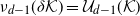 $\nu_{d-1}(\delta \mathcal{K})=\mathcal{U}_{d-1}(\mathcal{K})$ be the surface area of
  $\mathcal{K},$ where
  $\delta \mathcal{K}$ denotes the boundary of
  $\mathcal{K}.$ For
  $d=1,$ we put
  $\mathcal{U}_{0}(\mathcal{K})=0.$ For example, let
 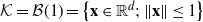 $\mathcal{K}=\mathcal{B}(1)=\left\{\mathbf{x}\in \mathbb{R}^{d};\ \|\mathbf{x}\|\leq 1\right\}$ be the unit ball. Hence,
  $\delta \mathcal{K}= \delta \mathcal{B}(1)=\mathcal{S}_{d-1}=\left\{ \mathbf{x}\in \mathbb{R}^{d};\ \|\mathbf{x}\|= 1\right\}$ is the unit sphere. Thus,
 \begin{equation}\mathcal{D}(\mathcal{B}(1))=2,\quad \left|\mathcal{B}(1)\right|=\frac{\pi^{d/2}}{\Gamma \!\left(\frac{d}{2}+1\right)},\ \mathcal{U}_{d-1}\!\left(\mathcal{B}(1)\right)=\left|\mathcal{S}_{d-1}\right|=\frac{2\pi^{\frac{d}{2}}}{\Gamma \!\left(\frac{d}{2}\right)}.\end{equation}
Let  $\mathcal{Q}$ be the stellate space in
  $\mathbb{R}^{d},$ and let
  $d\Gamma $ be an element of locally finite measure in the space
  $\mathcal{Q},$ which is invariant with respect to the group
  $\mathcal{M}$ of all Euclidean motions in the space
  $\mathbb{R}^{d}.$ Let now consider a chord length distribution function of the body
  $\mathcal{K},$ given by
 \begin{equation}F_{\mathcal{K}}(v)=\frac{2(d-1)}{\left|\mathcal{S}_{d-2}\right|}\int_{\chi(\Gamma )\leq v}d\Gamma,\end{equation}
where  $\chi(\Gamma )=\Gamma \cap\mathcal{K}$ is a chord in
  $\mathcal{K}.$ For example, if
  $\mathcal{K}=\mathcal{B}(1),$ then
 \begin{align}F_{\mathcal{B}(1)}(v)=\left\{\begin{array}{l}0,\quad v\leq 0,\\[2pt]
1-\left(1-\left(\frac{v}{2}\right)^{2}\right)^{\frac{d-1}{2}},\quad 0\leq v\leq 2,\\[8pt]
1,\quad v\geq 2\\\end{array}\right.\end{align}
\begin{align}F_{\mathcal{B}(1)}(v)=\left\{\begin{array}{l}0,\quad v\leq 0,\\[2pt]
1-\left(1-\left(\frac{v}{2}\right)^{2}\right)^{\frac{d-1}{2}},\quad 0\leq v\leq 2,\\[8pt]
1,\quad v\geq 2\\\end{array}\right.\end{align}
(see Ahoronyan and Khalatyan [Reference Aharonyan and Khalatyan2] for details).
Let now consider two points  $P_{1},P_{2}\in \mathcal{K}$, randomly and independently selected, with uniform distribution in
  $\mathcal{K}.$ We consider the probability density
  $\psi_{\rho_{\mathcal{K}}}$ of the random variable
 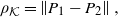 $\rho_{\mathcal{K}}=\left\|P_{1}-P_{2}\right\|,$ given by
 \begin{equation*}\psi_{\rho_{\mathcal{K}}}(z)=\frac{d}{dz}\mathbb{P}\!\left(\rho_{\mathcal{K}}\leq z\right). \end{equation*}
In the particular case  $\mathcal{K}=[{-}1,1],$
  $d=1,$ we have
 \begin{equation*}\psi_{\rho_{\mathcal{K}}}(u)=1-\frac{u}{2},\quad 0\leq u\leq 2,\end{equation*}
while for  $d\geq 2$ (see Ivanov and Leonenko [Reference Ivanov and Leonenko16] and Lord [Reference Lord28])
 \begin{equation} \psi_{\rho_{\mathcal{B}(1)}}(z)=\mathcal{I}_{1-\left(\frac{z}{2}\right)^{2}}\!\left(\frac{d+1}{2},\frac{1}{2}\right),\quad 0\leq z\leq 2, \end{equation}
where  $\mathcal{I}_{\mu}(p,q)$ denotes the incomplete beta function, given by
 \begin{equation}\mathcal{I}_{\mu}(p,q)=\frac{\Gamma (p+q)}{\Gamma (p)\Gamma (q)}\int_{0}^{\mu}t^{p-1}(1-t)^{q-1}dt,\quad \mu \in [0,1]. \end{equation}
It is also known (see, e.g., Equation (2.6) in Ahoronyan and Khalatyan [Reference Aharonyan and Khalatyan2]) that
 \begin{align}\psi_{\rho_{\mathcal{K}}}(z) & = \frac{1}{|\mathcal{K}|^{2}}\!\left[z^{d-1}\left| \mathcal{S}_{d-1}\right|\left| \mathcal{K}\right|\right.\nonumber\\
&- \left. z^{d-1}|\mathcal{S}_{d-2}|\mathcal{U}_{d-1}(\mathcal{K})\frac{1}{d-1}\int_{0}^{z}\!\left(1-F_{\mathcal{K}}(v)\right)dv\right],\quad 0\leq z\leq \mathcal{D}(\mathcal{K}).\end{align}
\begin{align}\psi_{\rho_{\mathcal{K}}}(z) & = \frac{1}{|\mathcal{K}|^{2}}\!\left[z^{d-1}\left| \mathcal{S}_{d-1}\right|\left| \mathcal{K}\right|\right.\nonumber\\
&- \left. z^{d-1}|\mathcal{S}_{d-2}|\mathcal{U}_{d-1}(\mathcal{K})\frac{1}{d-1}\int_{0}^{z}\!\left(1-F_{\mathcal{K}}(v)\right)dv\right],\quad 0\leq z\leq \mathcal{D}(\mathcal{K}).\end{align}
In particular, for the ball  $\mathcal{K}=\mathcal{B}(1),$ we obtain an alternative to Equation (4), given by, for
  $0\leq z\leq 2,$
 \begin{equation}\psi_{\rho_{\mathcal{B}(1)}}(z)=z^{d-1}\!\left[\frac{2\Gamma \!\left(\frac{d}{2}+1\right)}{\pi^{\frac{2d-1}{2}}}-\frac{4\Gamma \!\left(\frac{d}{2}+1\right)}{\pi^{\frac{d-1}{2}}\Gamma \!\left(\frac{d+1}{2}\right)(d-1)}\int_{0}^{z}\!\left(1-\left(\frac{u}{2}\right)^{2}\right)^{\frac{d-1}{2}}du\right].\end{equation}
3. Reduction theorems for spatiotemporal random fields with LRD in time
Let  $(\Omega ,\mathcal{A},\mathbb{P})$ be the basic probability space, where the random components of the spatiotemporal real-valued Gaussian random field
 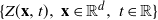 $\{Z(\mathbf{x},t),\ \mathbf{x}\in \mathbb{R}^{d},\ t\in \mathbb{R}\}$ are defined. That is,
  $Z\,:\,(\Omega ,\mathcal{A},\mathbb{P})\times \mathbb{R}^{d}\times \mathbb{R}\to \mathbb{R}.$
Condition 1. Let Z be a measurable Gaussian random field that is mean-square continuous, homogeneous and isotropic in space, and stationary in time, with  $\mathbb{E}[Z(\mathbf{x},t)]=0,$
  $\mathbb{E}[Z^{2}(\mathbf{x},t)]=1,$ and covariance function
  $\widetilde{C}(\|\mathbf{x}-\mathbf{y}\|,|t-s|)=\mathbb{E}\!\left[ Z(\mathbf{x},t)Z(\mathbf{y},s)\right]\geq 0,$ for every
  $t,s\in \mathbb{R}$ and
  $\mathbf{x}, \mathbf{y}\in \mathbb{R}^{d}.$ In spherical coordinates we write
 \begin{equation} C(z,\tau)=\widetilde{C}(\|\mathbf{x}-\mathbf{y}\|,|t-s|),\quad z=\|\mathbf{x}-\mathbf{y}\|\geq 0,\ \tau=|t-s|\geq 0. \end{equation}
For simplicity, we will use  $d\mathbf{x}$ instead of
  $\nu_{d}(d\mathbf{x}),$ and dt instead of
  $\nu(dt).$ In the case of spatiotemporal isotropic spherical random fields, sojourn functionals have been analyzed in Marinucci, Rossi and Vidotto [Reference Marinucci, Rossi and Vidotto32]. We now introduce the following sojourn functional, motivated by the first Minkowski functional. For each fixed time t, the random area
 \begin{align*} \mathcal{A}_{u}(t) & = \left|Z^{-1}(\cdot,t)\left( [u,\infty)\right)\right|=\left|\left\{\mathbf{x}\in \mathcal{K};\ Z(\mathbf{x},t)\geq u \right\}\right|\nonumber\\
& = \int_{\mathcal{K}}1_{\mathcal{S}_{Z}(u)}(\mathbf{x},t)d\mathbf{x}\nonumber \end{align*}
\begin{align*} \mathcal{A}_{u}(t) & = \left|Z^{-1}(\cdot,t)\left( [u,\infty)\right)\right|=\left|\left\{\mathbf{x}\in \mathcal{K};\ Z(\mathbf{x},t)\geq u \right\}\right|\nonumber\\
& = \int_{\mathcal{K}}1_{\mathcal{S}_{Z}(u)}(\mathbf{x},t)d\mathbf{x}\nonumber \end{align*}
provides the empirical measure (i.e., the excursion area) of  $Z(\cdot,t)$ corresponding to the level u,
  $u\in \mathbb{R}.$ The integrated area over the temporal interval [0, T] is then computed as
 \begin{equation} M_{T}^{(1)}(u)=\left|\left\{0\leq t\leq T;\ \mathbf{x}\in \mathcal{K},\ Z(\mathbf{x},t)\geq u\right\}\right|=\int_{0}^{T}\int_{\mathcal{K}}1_{\mathcal{S}_{Z}(u)} (\mathbf{x},t)d\mathbf{x}dt, \end{equation}
where  $1_{\mathcal{S}_{Z}(u)}(\cdot,\cdot)$ denotes the indicator function of the set
 \begin{equation*}\mathcal{S}_{Z}(u)=\{(\mathbf{y},s)\in \mathcal{K}\times [0,T];\ Z(\mathbf{y},s)\geq u\}.\end{equation*}
Similarly, we can define, for  $u\geq 0,$ the random area
 \begin{align} \mathcal{\widetilde{A}}_{u}(t) & = \left|Z^{-1}(\cdot,t)\left[ ({-}\infty,-u]\cup [u,\infty)\right]\right|=\left|\left\{\mathbf{x}\in \mathcal{K};\ \left| Z(\mathbf{x},t)\right|\geq u \right\}\right|\nonumber\\
& = \int_{\mathcal{K}}1_{\mathcal{S}_{|Z|}(u)}(\mathbf{x},t)d\mathbf{x},\nonumber \end{align}
\begin{align} \mathcal{\widetilde{A}}_{u}(t) & = \left|Z^{-1}(\cdot,t)\left[ ({-}\infty,-u]\cup [u,\infty)\right]\right|=\left|\left\{\mathbf{x}\in \mathcal{K};\ \left| Z(\mathbf{x},t)\right|\geq u \right\}\right|\nonumber\\
& = \int_{\mathcal{K}}1_{\mathcal{S}_{|Z|}(u)}(\mathbf{x},t)d\mathbf{x},\nonumber \end{align}
temporally integrated over [0, T], defining the functional
 \begin{equation} M_{T}^{(2)}(u)=\left|\left\{0\leq t\leq T;\ \mathbf{x}\in \mathcal{K},\ \left|Z(\mathbf{x},t)\right|\geq u \right\}\right|=\int_{0}^{T}\int_{\mathcal{K}}1_{\mathcal{S}_{|Z|}(u)} (\mathbf{x},t)d\mathbf{x}dt. \end{equation}
Let  $Z\sim \mathcal{N}(0,1)$ be a standard Gaussian random variable with probability density
  $\phi ,$ and distribution function
  $\Phi $ given by
 \begin{equation*}\phi (z)=\frac{1}{\sqrt{2\pi}}\exp\!\left({-}\frac{z^{2}}{2}\right),\quad \Phi (u)=\int_{-\infty }^{u}\phi_{Z}(z)dz,\quad z,u\in \mathbb{R}.\end{equation*}
Now let  $\mathcal{G}$ be a Borel measurable function such that
 \begin{equation*}\int_{\mathbb{R}}[\mathcal{G}(z)]^{2}\phi (z)dz<\infty.\end{equation*}
Then  $\mathcal{G}$ has an expansion with respect to the normalized Hermite polynomials that converges in
  $L_{2}(\mathbb{R}, \phi (z)dz ):$
 \begin{equation}\mathcal{G}(z)=\sum_{q=0}^{\infty }\frac{\mathcal{G}_{q}}{q!}H_{q}(z),\quad z\in \mathbb{R},\quad \mathcal{G}_{q}=\int_{\mathbb{R}}H_{q}(\xi)\mathcal{G}(\xi)\phi(\xi)d\xi,\quad q\geq 1,\end{equation}
where the Hermite polynomial of order  $q\geq 1,$ denoted by
  $H_{q}$, satisfies the equation
 \begin{equation}\frac{d^{n}\phi}{dz^{n}}(z)=({-}1)^{n}H_{n}(z)\phi(z).\end{equation}
Note that
 \begin{align}H_{0}(x) & = 1, H_{1}(x)=x, H_{2}(x)=x^{2}-1,\nonumber\\
H_{3}(x)& = x^{3}-3x, H_{4}(x)= x^{4}-6x^{2}+3,\dots.\end{align}
\begin{align}H_{0}(x) & = 1, H_{1}(x)=x, H_{2}(x)=x^{2}-1,\nonumber\\
H_{3}(x)& = x^{3}-3x, H_{4}(x)= x^{4}-6x^{2}+3,\dots.\end{align}
In particular, if  $\mathcal{G}_{u}(z)=1_{\{z\geq u\}},$ we then obtain
 \begin{align}\mathcal{G}_{u}(Z(\mathbf{x},t)) & = \mathbb{E}[1_{\mathcal{S}_{Z}(u)}(\mathbf{x},t)]\nonumber\\
& + \sum_{q=1}^{\infty }\frac{\mathcal{G}_{q}(u)}{q!}H_{q}(Z(\mathbf{x},t)),\quad \forall (\mathbf{x},t)\in \mathbb{R}^{d}\times \mathbb{R}.\end{align}
\begin{align}\mathcal{G}_{u}(Z(\mathbf{x},t)) & = \mathbb{E}[1_{\mathcal{S}_{Z}(u)}(\mathbf{x},t)]\nonumber\\
& + \sum_{q=1}^{\infty }\frac{\mathcal{G}_{q}(u)}{q!}H_{q}(Z(\mathbf{x},t)),\quad \forall (\mathbf{x},t)\in \mathbb{R}^{d}\times \mathbb{R}.\end{align}
Here, for every  $(\mathbf{x},t)\in \mathbb{R}^{d}\times \mathbb{R},$
 \begin{align}\mathcal{G}_{0}(u) & = \mathbb{E}\!\left[1_{ \mathcal{S}_{Z}(u) }(\mathbf{x},t)\right] = [1-\Phi(u)]=\int_{u }^{\infty}\phi(\xi)d\xi,\nonumber\\
\mathcal{G}_{q}(u) & = \phi(u)H_{q-1}(u),\quad q\geq 1.\end{align}
\begin{align}\mathcal{G}_{0}(u) & = \mathbb{E}\!\left[1_{ \mathcal{S}_{Z}(u) }(\mathbf{x},t)\right] = [1-\Phi(u)]=\int_{u }^{\infty}\phi(\xi)d\xi,\nonumber\\
\mathcal{G}_{q}(u) & = \phi(u)H_{q-1}(u),\quad q\geq 1.\end{align}
For the second functional, corresponding to  $\widetilde{\mathcal{G}}_{u}(z)=1_{\{\left|z\right|\geq u\}},$ we have
 \begin{align}\widetilde{\mathcal{G}}_{0}(u) & = \mathbb{E}[1_{\mathcal{S}_{|Z|}(u)}(\mathbf{x},t)] =2 [1-\Phi(u)]=2\int_{u}^{\infty}\phi(\xi)d\xi,\nonumber\\
\widetilde{\mathcal{G}}_{q}(u) & = 2\phi(u)H_{q-1}(u),\end{align}
\begin{align}\widetilde{\mathcal{G}}_{0}(u) & = \mathbb{E}[1_{\mathcal{S}_{|Z|}(u)}(\mathbf{x},t)] =2 [1-\Phi(u)]=2\int_{u}^{\infty}\phi(\xi)d\xi,\nonumber\\
\widetilde{\mathcal{G}}_{q}(u) & = 2\phi(u)H_{q-1}(u),\end{align}
for any even  $q\geq 0,$ and
  $\widetilde{\mathcal{G}}_{q}(u)=0$ for odd
  $q\geq 1.$
In what follows, from (14)–(16), we will consider the induced expansions of the functionals  $M_{T}^{(i)}(u),$
  $i=1,2,$ given by
 \begin{align}M_{T}^{(1)}(u) = (1-\Phi(u))T|\mathcal{K}|+\phi(u)\sum_{n=1}^{\infty}\frac{H_{n-1}(u)}{n!}\eta_{n},\end{align}
 \begin{align}M_{T}^{(2)}(u) = 2(1-\Phi(u))T|\mathcal{K}|+2\phi(u)\sum_{n=1}^{\infty}\frac{H_{2n-1}(u)}{(2n)!}\eta_{n},\end{align}
where
 \begin{align}\eta_{n} = \int_{0}^{T}\int_{\mathcal{K}}H_{n}(Z(\mathbf{x},t))d\mathbf{x}dt,\nonumber\end{align}
and
 \begin{align}\mathbb{E}[\eta_{n}]& = 0,\quad \mathbb{E}[\eta_{n}\eta_{l}]=0,\quad n\neq l,\nonumber\\
\sigma^{2}_{n,\mathcal{K}}(T) & = \mathbb{E}[\eta_{n}^{2}]=2n!T\int_{0}^{T}\!\left(1-\frac{\tau}{T}\right)\int_{\mathcal{K}\times \mathcal{K}}\widetilde{C}^{n}(\|\mathbf{x}-\mathbf{y}\|,\tau)d\tau d\mathbf{x}d\mathbf{y}\nonumber\\
& = 2n!T|\mathcal{K}|^{2}\int_{0}^{T}\!\left(1-\frac{\tau}{T}\right)\mathbb{E}\!\left[\widetilde{C}^{n}\!\left(\|P_{1}-P_{2}\|,\tau\right) \right]d\tau\nonumber\\
& = 2n!T|\mathcal{K}|^{2}\int_{0}^{T}\!\left(1-\frac{\tau}{T}\right)\int_{0}^{\mathcal{D}(\mathcal{K})}\psi_{\rho_{\mathcal{K}}}(z)C^{n}(z,\tau )dzd\tau.\end{align}
\begin{align}\mathbb{E}[\eta_{n}]& = 0,\quad \mathbb{E}[\eta_{n}\eta_{l}]=0,\quad n\neq l,\nonumber\\
\sigma^{2}_{n,\mathcal{K}}(T) & = \mathbb{E}[\eta_{n}^{2}]=2n!T\int_{0}^{T}\!\left(1-\frac{\tau}{T}\right)\int_{\mathcal{K}\times \mathcal{K}}\widetilde{C}^{n}(\|\mathbf{x}-\mathbf{y}\|,\tau)d\tau d\mathbf{x}d\mathbf{y}\nonumber\\
& = 2n!T|\mathcal{K}|^{2}\int_{0}^{T}\!\left(1-\frac{\tau}{T}\right)\mathbb{E}\!\left[\widetilde{C}^{n}\!\left(\|P_{1}-P_{2}\|,\tau\right) \right]d\tau\nonumber\\
& = 2n!T|\mathcal{K}|^{2}\int_{0}^{T}\!\left(1-\frac{\tau}{T}\right)\int_{0}^{\mathcal{D}(\mathcal{K})}\psi_{\rho_{\mathcal{K}}}(z)C^{n}(z,\tau )dzd\tau.\end{align}
Condition 2. Assume that
(i)
 $\sup_{z\in [0,\mathcal{D}(\mathcal{K})]}|C(z,\tau)|=\sup_{z\in [0,\mathcal{D}(\mathcal{K})]}C(z,\tau)\to 0,$ $\tau\to \infty$, and
-
(ii) for certain fixed
$m\in \{ 1,2,\dots\},$ there exists $\delta \in (0,1)$ such that
(20)
\begin{align}\lim_{T\to \infty}\frac{1}{T^{\delta }}\int_{0}^{T}\!\left(1-\frac{\tau}{T}\right)\int_{0}^{\mathcal{D}(\mathcal{K})}C^{m}(z,\tau)\psi_{\rho_{\mathcal{K}}}(z)dzd\tau=\infty.\end{align}


3.1. Reduction theorem
In this section, we extend the results of Taqqu [Reference Taqqu41, Reference Taqqu42] to the case of spatiotemporal random fields with LRD in time. For a function  $\mathcal{G}\in L_{2}(\mathbb{R},\phi(u)du),$ under Condition 1, we consider the following local functional:
 \begin{align} A_{T} & = \int_{0}^{T}\int_{\mathcal{K}}\mathcal{G}(Z(\mathbf{x},t))d\mathbf{x}dt\nonumber\\
& = T|\mathcal{K}|\mathcal{G}_{0}+\sum_{n=1}^{\infty}\frac{\mathcal{G}_{n}}{n!}\int_{0}^{T}\int_{\mathcal{K}}H_{n}(Z(\mathbf{x},t))d\mathbf{x}dt, \end{align}
\begin{align} A_{T} & = \int_{0}^{T}\int_{\mathcal{K}}\mathcal{G}(Z(\mathbf{x},t))d\mathbf{x}dt\nonumber\\
& = T|\mathcal{K}|\mathcal{G}_{0}+\sum_{n=1}^{\infty}\frac{\mathcal{G}_{n}}{n!}\int_{0}^{T}\int_{\mathcal{K}}H_{n}(Z(\mathbf{x},t))d\mathbf{x}dt, \end{align}
where, for  $n\geq 0,$
  $\mathcal{G}_{n}$ denotes the Fourier coefficient of the function
  $\mathcal{G}$ with respect to
  $H_{n},$ and the series (21) converges in
  $\mathcal{L}_{2}(\Omega,\mathcal{A},P).$ As in (19), let
  $\sigma^{2}_{n,\mathcal{K}}(T)=\mathbb{E}[\eta_{n}^{2}]$; then we obtain
 \begin{align} \sigma_{T}^{2}=\mbox{Var}(A_{T})=\mathbb{E}\!\left[A_{T}-E[A_{T}]\right]^{2}=\sum_{n=1}^{\infty }\sigma^{2}_{n,\mathcal{K}}(T).\nonumber \end{align}
Definition. We say that an integer  $m\geq 1$ is the Hermite rank of a function
  $\mathcal{G}$ if, for
  $m=1,$
  $\mathcal{G}_{1}\neq 0,$ or if, for
  $m\geq 2,$
  $\mathcal{G}_{1}=\dots =\mathcal{G}_{m-1}=0,$
  $\mathcal{G}_{m}\neq 0$ (see also Taqqu [Reference Taqqu41]).
Theorem 1. Under Conditions 1 and 2, assume that the function  $\mathcal{G}$ in (21) has Hermite rank
  $m;$ then the random variables
 \begin{align} Y_{T}=\frac{A_{T}-\mathbb{E}[A_{T}]}{|\mathcal{G}_{m}|\sigma_{m,\mathcal{K}}(T)(1/m!)} \end{align}
and
 \begin{align} Y_{m,T}=\frac{\mbox{sgn}\{\mathcal{G}_{m}\}\int_{0}^{T}\int_{\mathcal{K}}H_{m}(Z(\mathbf{x},t))d\mathbf{x}dt}{\sigma_{m,\mathcal{K}}(T)} \end{align}
have the same limiting distribution (if one exists).
Proof. We split
 \begin{equation*}A_{T}-\mathbb{E}[A_{T}]=S_{1,T}+S_{2,T},\end{equation*}
where, using the notation (19) and applying Parseval’s identity,
 \begin{align} S_{1,T}=\frac{\mathcal{G}_{m}}{m!}\xi_{m},\qquad S_{2,T}=\sum_{n=m+1}^{\infty}\frac{\mathcal{G}_{n}}{n!}\xi_{n},\qquad \sum_{n=m}^{\infty } \frac{\mathcal{G}^{2}_{n}}{n!}<\infty\quad \mbox{almost surely}. \end{align}
 \begin{equation} \mbox{Var}\!\left( A_{T}\right)=\mbox{Var}(S_{1,T})+\mbox{Var}(S_{2,T}), \end{equation}
and we have to show that
 \begin{equation*}\frac{\mbox{Var}(S_{2,T})}{\sigma^{2}_{m,\mathcal{K}}(T)}\to 0,\quad T\to \infty.\end{equation*}
Under Condition 2(i),
 \begin{equation} \sup_{z\in [0,\mathcal{D}(\mathcal{K})], \tau\geq T^{\delta}} C(z,\tau )\to 0,\quad T\to \infty, \end{equation}
where  $\delta $ satisfies Condition 2(ii). Note that, for
  $0\leq \tau\leq T^{\delta},$ the unit variance of Z allows us to work with the uniform estimate
  $|C(z,\tau)|^{m+1}\leq 1,$
  $z\in \mathbb{R}_{+}.$ From (24), we then have
 \begin{align} \mbox{Var}(S_{2,T})&\leq \sum_{n=m+1}^{\infty}\frac{\mathcal{G}_{n}^{2}}{(n!)^{2}}\sigma_{n,\mathcal{K}}^{2}(T)\nonumber\\
&\leq M_{1}\!\left\{2T\!\left[\int_{0}^{T^{\delta }}+\int_{T^{\delta }}^{T}\right]\right\}\left(1-\frac{\tau}{T}\right)\int_{0}^{\mathcal{D}(\mathcal{K})}C^{m+1}(z,\tau) \psi_{\rho_{\mathcal{K}}}(z)dzd\tau, \nonumber \end{align}
\begin{align} \mbox{Var}(S_{2,T})&\leq \sum_{n=m+1}^{\infty}\frac{\mathcal{G}_{n}^{2}}{(n!)^{2}}\sigma_{n,\mathcal{K}}^{2}(T)\nonumber\\
&\leq M_{1}\!\left\{2T\!\left[\int_{0}^{T^{\delta }}+\int_{T^{\delta }}^{T}\right]\right\}\left(1-\frac{\tau}{T}\right)\int_{0}^{\mathcal{D}(\mathcal{K})}C^{m+1}(z,\tau) \psi_{\rho_{\mathcal{K}}}(z)dzd\tau, \nonumber \end{align}
for  $M_{1}>0,$ whose value follows from (19). In addition, from (6),
 \begin{equation} \psi_{\rho_{\mathcal{K}}}(z)\leq \frac{z^{d-1}}{|\mathcal{K}|}|S_{d-1}|,\qquad 0\leq z\leq \mathcal{D}(\mathcal{K}), \end{equation}
leading to
 \begin{align} \mbox{Var}(S_{2,T})&\leq M_{1}\!\left\{M_{2}T^{\delta +1}+2T\int_{T^{\delta }}^{T}\!\left(1-\frac{\tau}{T}\right)\int_{\mathcal{K}}C^{m+1}(z,\tau) \psi_{\rho_{\mathcal{K}}}(z)dzd\tau\right\}\nonumber\\[3pt]
&\leq M_{3}\!\left\{T^{\delta +1}+2T\sup_{z\in [0,\mathcal{D}(\mathcal{K})], \tau \geq T^{\delta }}C(z,\tau)\right.\nonumber\\[3pt]
& \qquad\qquad\qquad\left.\times \int_{T^{\delta }}^{T}\!\left(1-\frac{\tau}{T}\right)\int_{\mathcal{K}}C^{m}(z,\tau) \psi_{\rho_{\mathcal{K}}}(z)dzd\tau\right\}. \end{align}
\begin{align} \mbox{Var}(S_{2,T})&\leq M_{1}\!\left\{M_{2}T^{\delta +1}+2T\int_{T^{\delta }}^{T}\!\left(1-\frac{\tau}{T}\right)\int_{\mathcal{K}}C^{m+1}(z,\tau) \psi_{\rho_{\mathcal{K}}}(z)dzd\tau\right\}\nonumber\\[3pt]
&\leq M_{3}\!\left\{T^{\delta +1}+2T\sup_{z\in [0,\mathcal{D}(\mathcal{K})], \tau \geq T^{\delta }}C(z,\tau)\right.\nonumber\\[3pt]
& \qquad\qquad\qquad\left.\times \int_{T^{\delta }}^{T}\!\left(1-\frac{\tau}{T}\right)\int_{\mathcal{K}}C^{m}(z,\tau) \psi_{\rho_{\mathcal{K}}}(z)dzd\tau\right\}. \end{align}
Hence,
 \begin{align}\frac{ \mbox{Var}(S_{2,T})}{\sigma_{m,\mathcal{K}}^{2}(T)}&\leq M_{4}\!\left\{\frac{1}{T^{-(\delta +1)}\sigma_{m,\mathcal{K}}^{2}(T)}\right.\nonumber\\
&\quad \left.+\, M_{5}\sup_{z\in [0,\mathcal{D}(\mathcal{K})], \tau\geq T^{\delta}}C(z,\tau)\frac{\int_{T^{\delta }}^{T}\left(1-\frac{\tau}{T}\right)\int_{\mathcal{K}}C^{m}(z,\tau) \psi_{\rho_{\mathcal{K}}}(z)dzd\tau}{\int_{0}^{T}\left(1-\frac{\tau}{T}\right)\int_{\mathcal{K}}C^{m}(z,\tau) \psi_{\rho_{\mathcal{K}}}(z)dzd\tau}\right\}.\nonumber \end{align}
\begin{align}\frac{ \mbox{Var}(S_{2,T})}{\sigma_{m,\mathcal{K}}^{2}(T)}&\leq M_{4}\!\left\{\frac{1}{T^{-(\delta +1)}\sigma_{m,\mathcal{K}}^{2}(T)}\right.\nonumber\\
&\quad \left.+\, M_{5}\sup_{z\in [0,\mathcal{D}(\mathcal{K})], \tau\geq T^{\delta}}C(z,\tau)\frac{\int_{T^{\delta }}^{T}\left(1-\frac{\tau}{T}\right)\int_{\mathcal{K}}C^{m}(z,\tau) \psi_{\rho_{\mathcal{K}}}(z)dzd\tau}{\int_{0}^{T}\left(1-\frac{\tau}{T}\right)\int_{\mathcal{K}}C^{m}(z,\tau) \psi_{\rho_{\mathcal{K}}}(z)dzd\tau}\right\}.\nonumber \end{align}
From (19), under Condition 2(ii),
 \begin{align} \frac{\sigma_{m,\mathcal{K}}^{2}(T)}{T^{\delta +1}}\to \infty,\quad T\to \infty, \end{align}
and under Condition 2(i),
 \begin{equation*}\sup_{z\in [0,\mathcal{D}(\mathcal{K})], \tau\geq T^{\delta}}C(z,\tau)\to 0,\quad T\to \infty.\end{equation*}
Note that
 \begin{equation} \frac{\int_{T^{\delta }}^{T}\!\left(1-\frac{\tau}{T}\right)\int_{\mathcal{K}}C^{m}(z,\tau) \psi_{\rho_{\mathcal{K}}}(z)dzd\tau}{\int_{0}^{T}\!\left(1-\frac{\tau}{T}\right)\int_{\mathcal{K}}C^{m}(z,\tau) \psi_{\rho_{\mathcal{K}}}(z)dzd\tau}\leq 1. \end{equation}
The convergence to zero of
 \begin{equation*}\frac{ \mbox{Var}(S_{2,T})}{\sigma_{m,\mathcal{K}}^{2}(T)}\end{equation*}
then follows from Equation (29) under Condition 2, leading to
 \begin{equation*}\mathbb{E}[Y_{T}-Y_{m,T}]^{2}=\frac{ \mbox{\small Var}(S_{2,T})}{\sigma_{m,\mathcal{K}}^{2}(T)}\to 0, \qquad T\to \infty,\end{equation*}
as we wanted to prove.
Remark 1. We have applied in (30) that, under Condition 1, the correlation function  $C(z,\tau)\geq 0,$ for every
  $\tau ,z\in \mathbb{R}_{+}.$
Remark 2. For a short-memory case, one can assume that for a fixed  $m\geq 1,$
 \begin{equation*}\int_{0}^{\infty}\int_{0}^{\mathcal{D}(\mathcal{K})} \psi_{\rho_{\mathcal{K}}}(\mathbf{z})\left|C(\mathbf{z},\tau)\right|^{m}d\mathbf{z}d\tau <\infty.\end{equation*}
Then one can show using standard arguments that as  $T\to \infty,$ the asymptotic variance satisfies
 \begin{equation}\sigma_{T}^{2}=\mbox{Var}(A_{T})=\sum_{n=m}^{\infty }\frac{\mathcal{G}_{n}^{2}}{(n!)^{2}}\sigma^{2}_{n,\mathcal{K}}(T)=TB(1+o(1)),\end{equation}
where
 \begin{equation*}B=\sum_{n=m}^{\infty}\frac{\mathcal{G}_{n}^{2}}{(n!)^{2}}\lim_{T\to \infty}\frac{\sigma^{2}_{n,\mathcal{K}}(T)}{T}<\infty.\end{equation*}
Then, using the method of moments and diagram formulae (for details see Theorem 2.3.1 in Ivanov and Leonenko [Reference Ivanov and Leonenko16]), one can prove under the condition (31) that  $(A_{T}-E[A_{T}])/\sqrt{T}$ converges to a normal distribution with zero mean and variance B.
4. Sojourn functionals
As an application of the reduction result, Theorem 1, the following result proves the convergence to a standard normal distribution for the case of Hermite rank  $m=1.$
Theorem 2. Under Conditions 1 and 2, for  $m=1,$ the random variables
 \begin{align}&&X_{1,T}=\frac{M_{T}^{(1)}(u)-T|\mathcal{K}|(1-\Phi(u))}{\phi(u)\left[2T\int_{0}^{T}\!\left(1-\frac{\tau }{T}\right)\int_{0}^{\mathcal{D}(\mathcal{K})} C(z,\tau)\psi_{\rho_{\mathcal{K}}}(z)dzd\tau\right]^{1/2}}\nonumber\end{align}
and
 \begin{align}\frac{\int_{0}^{T}\int_{\mathcal{K}}Z(x,t)dxdt}{\left[2T\int_{0}^{T}\!\left(1-\frac{\tau }{T}\right)\int_{0}^{\mathcal{D}(\mathcal{K})}C(z,\tau)\psi_{\rho_{\mathcal{K}}}(z)dzd\tau\right]^{1/2}}\end{align}
have the same limit as  $T\to \infty.$ Namely, the convergence to a standard normal distribution holds.
We now formulate the result analogous to Theorem 2 for the functional  $M_{T}^{(2)}$.
Theorem 3. Under Conditions 1 and 2, with  $m=2,$ the random variables
 \begin{align} &&X_{2,T}=\frac{M_{T}^{(2)}(u)-2T|\mathcal{K}|(1-\Phi(u))}{[\phi(u)]^{2}\!\left[T|\mathcal{K}|^{2}\int_{0}^{T}\!\left(1-\frac{\tau }{T}\right)\int_{0}^{\mathcal{D}(\mathcal{K})} C^{2}(z,\tau)\psi_{\rho_{\mathcal{K}}}(z)dzd\tau\right]^{1/2}}\nonumber \end{align}
and
 \begin{align}&&Y_{2,T}=\frac{\int_{0}^{T}\int_{\mathcal{K}}(Z^{2}(x,t)-1)dxdt}{2\!\left[T|\mathcal{K}|^{2}\int_{0}^{T}\!\left(1-\frac{\tau }{T}\right)\int_{0}^{\mathcal{D}(\mathcal{K})}C^{2}(z,\tau)\psi_{\rho_{\mathcal{K}}}(z)dzd\tau\right]^{1/2}}\end{align}
have the same limit distribution, in the sense that if one exists then so does the other, and the two are equal.
5. Examples
In Sections 5.1 and 5.2, we will present some examples of covariance functions displaying LRD in time for which Conditions 2(i)–(ii) hold true.
5.1. Separable covariance structures
Under Condition 1, the covariance function  $\widetilde{C}(\|\mathbf{x}-\mathbf{y}\|,|t-s|)=C(z,\tau)$ is said to be separable if it can be factored as the product of a spatial covariance function
  $C_{\mathcal{S}}$ and a temporal covariance function
  $C_{\mathcal{T}}$ (see Cressie and Huang [Reference Cressie and Huang8] and Christakos [Reference Christakos7]). That is,
 \begin{equation}\widetilde{C}(\|\mathbf{x}-\mathbf{y}\|,|t-s|)=C(z,\tau)= C_{\mathcal{S}}(z)C_{\mathcal{T}}(\tau ), \end{equation}
where, as before,  $z\geq 0,$ and
  $\tau\geq 0.$
Condition 4. Consider the covariance function
 \begin{equation} C_{\mathcal{T}}(\tau )= \frac{\mathcal{L}(\tau )}{\tau^{\alpha }},\quad \tau \geq 0,\quad \alpha \in (0,1), \end{equation}
where  $\mathcal{L}$ is a function that is slowly varying at infinity and locally bounded, i.e., bounded on each bounded interval.
Under Conditions 1 and 4, for  $\alpha \in \left(0,\frac{1}{n}\right),$ for separable covariance functions as given in (34), we obtain
 \begin{align} \sigma_{n}^{2}(T) & = 2n! T\int_{0}^{T}\!\left(1-\frac{\tau }{T}\right)C^{n}_{\mathcal{T}}(\tau )d\tau\nonumber\\
& = T^{2-n\alpha }\mathcal{L}^{n}(T)\!\left[2n!\int_{0}^{1}(1-\tau)\tau^{-n\alpha }d\tau\right] \left( 1+o(1)\right). \end{align}
\begin{align} \sigma_{n}^{2}(T) & = 2n! T\int_{0}^{T}\!\left(1-\frac{\tau }{T}\right)C^{n}_{\mathcal{T}}(\tau )d\tau\nonumber\\
& = T^{2-n\alpha }\mathcal{L}^{n}(T)\!\left[2n!\int_{0}^{1}(1-\tau)\tau^{-n\alpha }d\tau\right] \left( 1+o(1)\right). \end{align}
From (19) and (36), as  $T\to \infty,$
 \begin{align} \sigma_{n,\mathcal{K}}^{2}(T) = c_{\mathcal{K}}(n,\alpha )T^{2-n\alpha }\mathcal{L}^{n}(T)\left( 1+o(1)\right),\nonumber\end{align}
where
 \begin{equation*}c_{\mathcal{K}}(n,\alpha )= 2n!\left[\int_{0}^{1}\!\left(1-\tau \right)\frac{d\tau }{\tau^{\alpha n}}\right]|\mathcal{K}|^{2}\int_{0}^{\mathcal{D}(\mathcal{K})} C_{\mathcal{S}}(z)\psi_{\rho_{\mathcal{K}}}(z)dz.\end{equation*}
Proposition 1. Under Conditions 1 and 4, for separable covariance functions (34), Condition 2(ii) holds for  $\alpha \in (0,1)$ if
  $m=1,$ and for
  $\alpha \in (0,1/2)$ if
  $m=2.$ Moreover, for
  $\alpha \in (0,1/2),$
the two random variables in (33) have the same limit distribution
$\alpha \in (0,1/2),$
the two random variables in (33) have the same limit distribution  $\mathcal{R}$ (as
  $T\rightarrow \infty$) of Rosenblatt type, given by the following Wiener–Itô integral representation, with respect to spatiotemporal complex Gaussian white noise random measure W on
  $\mathbb{R}^{2}\times \mathbb{R}^{2d}$ (integration over hyperdiagonals is excluded; see, e.g., Dobrushin and Major [Reference Dobrushin and Major9]):
 \begin{align}\mathcal{R} & = \frac{c_{T}(\alpha )}{\sqrt{c_{\mathcal{K}}(2,\alpha )}}\int_{\mathbb{R}^{2}}^{\prime }\frac{\exp \{i(\mu _{1}+\mu _{2})\}-1}{i(\mu _{1}+\mu _{2})}\frac{1}{\left\vert\mu _{1}\mu _{2}\right\vert ^{\frac{1-\alpha }{2}}}\nonumber\\
&\times \int_{\mathbb{R}^{2d}}^{\prime }\left[\int_{\mathcal{K}}\exp \!\left\{i\!\left\langle \mathbf{x},\boldsymbol{\omega}_{1}+\boldsymbol{\omega}_{2}\right\rangle\right\}d\mathbf{x}\right]\left[\prod_{j=1}^{2}f_{S}(\boldsymbol{\omega} _{j})\right]^{1/2}\nonumber\\
& \qquad\qquad\qquad\qquad\times W(d\mu_{1},d\boldsymbol{\omega} _{1})W(d\mu _{2},d\boldsymbol{\omega} _{2}),\end{align}
\begin{align}\mathcal{R} & = \frac{c_{T}(\alpha )}{\sqrt{c_{\mathcal{K}}(2,\alpha )}}\int_{\mathbb{R}^{2}}^{\prime }\frac{\exp \{i(\mu _{1}+\mu _{2})\}-1}{i(\mu _{1}+\mu _{2})}\frac{1}{\left\vert\mu _{1}\mu _{2}\right\vert ^{\frac{1-\alpha }{2}}}\nonumber\\
&\times \int_{\mathbb{R}^{2d}}^{\prime }\left[\int_{\mathcal{K}}\exp \!\left\{i\!\left\langle \mathbf{x},\boldsymbol{\omega}_{1}+\boldsymbol{\omega}_{2}\right\rangle\right\}d\mathbf{x}\right]\left[\prod_{j=1}^{2}f_{S}(\boldsymbol{\omega} _{j})\right]^{1/2}\nonumber\\
& \qquad\qquad\qquad\qquad\times W(d\mu_{1},d\boldsymbol{\omega} _{1})W(d\mu _{2},d\boldsymbol{\omega} _{2}),\end{align}
where
 \begin{equation*}f_{\mathcal{S}}(\boldsymbol{\omega })=\frac{1}{[2\pi]^{d}}\int_{\mathbb{R}^{d}}\exp\!\left({-}i\!\left\langle \boldsymbol{\omega },\mathbf{x}\right\rangle\right) \widetilde{C}_{\mathcal{S}}(\|\mathbf{x}\|) d\mathbf{x},\end{equation*}
and
 \begin{equation}c_{T}(\alpha )=\frac{\Gamma \!\left(\frac{1-\alpha }{2}\right)}{2^{\alpha }\Gamma \!\left(\frac{\alpha }{2}\right)\sqrt{\pi}} \end{equation}
is the Tauberian constant.
Remark 3. Note that  $E\!\left[\mathcal{R}^{2}\right]<\infty .$
Proof. The proof of Proposition 1 is standard (see, e.g., Leonenko and Olenko [Reference Leonenko and Olenko22]). A sketch of the proof is now given. Note that the spectral density of a spatiotemporal random field with separable covariance function (34) is also separable, i.e.,
 \begin{align} f(\boldsymbol{\omega },\mu) & = \frac{1}{(2\pi)^{d+1}}\int_{\mathbb{R}\times \mathbb{R}^{d}}\exp\!\left({-}i\mu\tau\right) \exp\!\left({-}i\!\left\langle \boldsymbol{\omega },\mathbf{x}\right\rangle\right)\widetilde{C}_{\mathcal{S}}(\|\mathbf{x}\|)\widetilde{C}_{\mathcal{T}}(|\tau|)d\mathbf{x}d\tau\nonumber\\[4pt]
& = \left[\frac{1}{[2\pi]^{d}}\int_{\mathbb{R}^{d}}\exp\!\left({-}i\!\left\langle \boldsymbol{\omega },\mathbf{x}\right\rangle\right) \widetilde{C}_{\mathcal{S}}(\|\mathbf{x}\|) d\mathbf{x}\right]\left[\frac{1}{2\pi}\int_{\mathbb{R}}\exp\!\left({-}i\mu\tau\right)\widetilde{C}_{\mathcal{T}}(|\tau|)d\tau\right]\nonumber\\[4pt]
& = f_{\mathcal{S}}(\boldsymbol{\omega })f_{\mathcal{T}}(\mu ),\quad \boldsymbol{\omega }\in \mathbb{R}^{d},\quad \mu \in \mathbb{R}. \end{align}
\begin{align} f(\boldsymbol{\omega },\mu) & = \frac{1}{(2\pi)^{d+1}}\int_{\mathbb{R}\times \mathbb{R}^{d}}\exp\!\left({-}i\mu\tau\right) \exp\!\left({-}i\!\left\langle \boldsymbol{\omega },\mathbf{x}\right\rangle\right)\widetilde{C}_{\mathcal{S}}(\|\mathbf{x}\|)\widetilde{C}_{\mathcal{T}}(|\tau|)d\mathbf{x}d\tau\nonumber\\[4pt]
& = \left[\frac{1}{[2\pi]^{d}}\int_{\mathbb{R}^{d}}\exp\!\left({-}i\!\left\langle \boldsymbol{\omega },\mathbf{x}\right\rangle\right) \widetilde{C}_{\mathcal{S}}(\|\mathbf{x}\|) d\mathbf{x}\right]\left[\frac{1}{2\pi}\int_{\mathbb{R}}\exp\!\left({-}i\mu\tau\right)\widetilde{C}_{\mathcal{T}}(|\tau|)d\tau\right]\nonumber\\[4pt]
& = f_{\mathcal{S}}(\boldsymbol{\omega })f_{\mathcal{T}}(\mu ),\quad \boldsymbol{\omega }\in \mathbb{R}^{d},\quad \mu \in \mathbb{R}. \end{align}
From Tauberian theorems (see Leonenko and Olenko [Reference Leonenko and Olenko23]), under Condition 4, we get the convergence
 \begin{equation} f_{\mathcal{T}}(\mu )\sim c_{T}(\alpha )\frac{\mathcal{L}\!\left(\frac{1}{\mu}\right)}{|\mu|^{1-\alpha }},\quad \mu\to 0, \end{equation}
for  $0<\alpha <\frac{1}{2},$ where the Tauberian constant
  $c_{T}(\alpha )$ has been introduced in (38). From (39), applying the Wiener–Itô stochastic integral representation (see, e.g., Major [Reference Major29] and Section 4.4.2 in Marinucci and Peccati [Reference Marinucci and Peccati31]), we obtain the isonormal representation
 \begin{equation} Z(\mathbf{x},t)=\int_{\mathbb{R}^{d}}\int_{\mathbb{R}}\exp\!\left(i\mu t\right)\exp\!\left(i\!\left\langle \boldsymbol{\omega},\mathbf{x}\right\rangle\right)\sqrt{f_{\mathcal{T}}(\mu )f_{\mathcal{S}}(\boldsymbol{\omega })}W(d\mu,d\boldsymbol{\omega }),\end{equation}
with W denoting the complex-valued white noise measure.
For  $\underset{d}{=}$ denoting the identity in probability distribution, applying now the self-similarity of the Gaussian white noise random measure,
 \begin{align}&& W(a d\mu,b d\boldsymbol{\omega })\underset{d}{=}\sqrt{a}b^{d/2}W(d\mu,d\boldsymbol{\omega }),\quad \forall \mu\in \mathbb{R},\ \boldsymbol{\omega}\in \mathbb{R}^{d}, \end{align}
and the Itô formula (see, e.g., Dobrushin and Major [Reference Dobrushin and Major9] and Major [Reference Major29]), from Equation (41), we obtain
 \begin{align}& Y_{2,T} =\frac{\int_{0}^{T}\int_{\mathcal{K}}\!\left(Z^{2}(\mathbf{x},t)-1\right)d\mathbf{x}dt}{T^{1-\alpha }\mathcal{L}(T)\sqrt{c_{\mathcal{K}}(2,\alpha )}}\nonumber\\
&\underset{d}{=} \int_{\mathbb{R}^{2}}^{\prime }\left[\int_{0}^{1}\exp\!\left(i(\mu_{1}+\mu_{2})t\right)dt\right]\left[\prod_{j=1}^{2}f_{\mathcal{T}} \!\left(\frac{\mu_{j}}{T}\right)\right]^{1/2}\frac{1}{T^{1-\alpha }\mathcal{L}(T)\sqrt{c_{\mathcal{K}}(2,\alpha )}}\nonumber\\
&\times\int_{\mathbb{R}^{2d}}^{\prime }\left[\int_{\mathcal{K}}\exp\!\left(i\!\left\langle\mathbf{x},\boldsymbol{\omega }_{1}+\boldsymbol{\omega}_{2}\right\rangle\right)d\mathbf{x}\right]\left[\prod_{j=1}^{2}f_{\mathcal{S}}(\boldsymbol{\omega}_{j})\right]^{1/2} W\!\left(d\mu_{1}, d\boldsymbol{\omega}_{1}\right)W\!\left(d\mu_{2}, d\boldsymbol{\omega}_{2}\right).\nonumber\\ \end{align}
\begin{align}& Y_{2,T} =\frac{\int_{0}^{T}\int_{\mathcal{K}}\!\left(Z^{2}(\mathbf{x},t)-1\right)d\mathbf{x}dt}{T^{1-\alpha }\mathcal{L}(T)\sqrt{c_{\mathcal{K}}(2,\alpha )}}\nonumber\\
&\underset{d}{=} \int_{\mathbb{R}^{2}}^{\prime }\left[\int_{0}^{1}\exp\!\left(i(\mu_{1}+\mu_{2})t\right)dt\right]\left[\prod_{j=1}^{2}f_{\mathcal{T}} \!\left(\frac{\mu_{j}}{T}\right)\right]^{1/2}\frac{1}{T^{1-\alpha }\mathcal{L}(T)\sqrt{c_{\mathcal{K}}(2,\alpha )}}\nonumber\\
&\times\int_{\mathbb{R}^{2d}}^{\prime }\left[\int_{\mathcal{K}}\exp\!\left(i\!\left\langle\mathbf{x},\boldsymbol{\omega }_{1}+\boldsymbol{\omega}_{2}\right\rangle\right)d\mathbf{x}\right]\left[\prod_{j=1}^{2}f_{\mathcal{S}}(\boldsymbol{\omega}_{j})\right]^{1/2} W\!\left(d\mu_{1}, d\boldsymbol{\omega}_{1}\right)W\!\left(d\mu_{2}, d\boldsymbol{\omega}_{2}\right).\nonumber\\ \end{align}
We define
 \begin{align} &\mathcal{I}_{\mathcal{K}}=\frac{1}{c_{\mathcal{K}}(2,\alpha )}\int_{\mathbb{R}^{2d}}\!\left|\int_{\mathcal{K}}\exp\!\left(i\!\left\langle\mathbf{x},\boldsymbol{\omega }_{1}+\boldsymbol{\omega}_{2}\right\rangle\right)d\mathbf{x}\right|^{2} \left[\prod_{j=1}^{2}f_{\mathcal{S}}(\boldsymbol{\omega}_{j})\right] d\boldsymbol{\omega}_{1}d\boldsymbol{\omega}_{2}\nonumber\\
&= \frac{|\mathcal{K}|^{2}}{c_{\mathcal{K}}(2,\alpha )}\mathbb{E}\!\left[C^{2}_{\mathcal{S}}\!\left(\|P_{1}-P_{2}\|\right)\right]\nonumber\\
&=\frac{|\mathcal{K}|^{2}}{c_{\mathcal{K}}(2,\alpha )}\int_{0}^{\mathcal{D}(\mathcal{K})}C^{2}_{\mathcal{S}}\!\left(z\right)\psi_{\rho_{\mathcal{K}}}(z)dz, \end{align}
\begin{align} &\mathcal{I}_{\mathcal{K}}=\frac{1}{c_{\mathcal{K}}(2,\alpha )}\int_{\mathbb{R}^{2d}}\!\left|\int_{\mathcal{K}}\exp\!\left(i\!\left\langle\mathbf{x},\boldsymbol{\omega }_{1}+\boldsymbol{\omega}_{2}\right\rangle\right)d\mathbf{x}\right|^{2} \left[\prod_{j=1}^{2}f_{\mathcal{S}}(\boldsymbol{\omega}_{j})\right] d\boldsymbol{\omega}_{1}d\boldsymbol{\omega}_{2}\nonumber\\
&= \frac{|\mathcal{K}|^{2}}{c_{\mathcal{K}}(2,\alpha )}\mathbb{E}\!\left[C^{2}_{\mathcal{S}}\!\left(\|P_{1}-P_{2}\|\right)\right]\nonumber\\
&=\frac{|\mathcal{K}|^{2}}{c_{\mathcal{K}}(2,\alpha )}\int_{0}^{\mathcal{D}(\mathcal{K})}C^{2}_{\mathcal{S}}\!\left(z\right)\psi_{\rho_{\mathcal{K}}}(z)dz, \end{align}
where in the last identity we have applied steps similar to (19).
From (43) and (44), we then obtain
 \begin{align} &&\mathbb{E}\!\left[Y_{2,T}-\mathcal{R} \right]^{2}=[c_{T}(\alpha )]^{2}\mathcal{I}_{\mathcal{K}}\int_{\mathbb{R}^{2}}\!\left|\int_{0}^{1}\exp\!\left(i(\mu_{1}+\mu_{2})t\right)dt\right|^{2} \nonumber\\ &&\times \frac{1}{|\mu_{1}\mu_{2}|^{1-\alpha }}Q_{T}(\mu_{1},\mu_{2})d\mu_{1}d\mu_{2}, \end{align}
where
 \begin{align} Q_{T}(\mu_{1},\mu_{2})=\left(\frac{1}{c_{T}(\alpha )}|\mu_{1}\mu_{2}|^{\frac{1-\alpha}{2} }\prod_{j=1}^{2}f_{\mathcal{T}}^{1/2}\left(\frac{\mu_{j}}{T}\right)\frac{1}{T^{1-\alpha }\mathcal{L}(T)}-1\right)^{2}. \end{align}
Applying Tauberian theorems (see (40)) and the dominated convergence theorem, we find that as  $T\to \infty,$ (45) converges to zero for
  $\alpha \in (0,1/2).$ Hence, the convergence in probability distribution of the random variable
  $Y_{2,T}$ to
  $\mathcal{R}$ holds (see Leonenko and Olenko [Reference Leonenko and Olenko22] for more details).
5.2. Nonseparable covariance functions
Let  $\varphi (v)\geq 0$ be a completely monotone function, that is, an infinite differentiable function satisfying
 \begin{equation*}({-}1)^{n}\frac{d^{n}\varphi}{dv^{n}}(v)\geq 0,\quad v>0,\quad n\geq 0.\end{equation*}
By Bernstein’s theorem,
 \begin{equation*} \varphi (v)=\int_{0}^{\infty} \exp\!\left({-}v\xi\right)\mu(d\xi),\end{equation*}
where  $\mu $ is a positive measure over
  $[0,\infty)$ (see Gneiting [Reference Gneiting13]).
Suppose further that  $\psi \,:\,[0,\infty)\to[0,\infty)$ has completely monotone derivatives, i.e., it is a Bernstein function. The Gneiting class of spatiotemporal covariance functions is defined as follows (see Gneiting [Reference Gneiting13]):
 \begin{align}\widetilde{C}(\left\Vert \mathbf{x}-\mathbf{y}\right\Vert ,|t-s|)& = \frac{1}{[\psi (|t-s|^{2})]^{d/2}}\varphi \!\left( \frac{\left\Vert \mathbf{x}-\mathbf{y}\right\Vert ^{2}}{\psi (|t-s|^{2})}\right) \nonumber\\
& = C(z,\tau)=\frac{1}{[\psi (\tau ^{2})]^{d/2}}\varphi \!\left( \frac{z ^{2}}{\psi (\tau^{2})}\right), \nonumber\\
& \quad \mathbf{x},\mathbf{y}\in \mathbb{R}^{d},\ t,s\in \mathbb{R}, \ \tau, z\geq 0.\end{align}
\begin{align}\widetilde{C}(\left\Vert \mathbf{x}-\mathbf{y}\right\Vert ,|t-s|)& = \frac{1}{[\psi (|t-s|^{2})]^{d/2}}\varphi \!\left( \frac{\left\Vert \mathbf{x}-\mathbf{y}\right\Vert ^{2}}{\psi (|t-s|^{2})}\right) \nonumber\\
& = C(z,\tau)=\frac{1}{[\psi (\tau ^{2})]^{d/2}}\varphi \!\left( \frac{z ^{2}}{\psi (\tau^{2})}\right), \nonumber\\
& \quad \mathbf{x},\mathbf{y}\in \mathbb{R}^{d},\ t,s\in \mathbb{R}, \ \tau, z\geq 0.\end{align}
It is known that the one-parameter Mittag-Leffler function  $E_{\nu},$ for
  $0<\nu \leq 1,$ is a completely monotone function (see Feller [Reference Feller12], p. 147), given by
 \begin{equation*}E_{\nu }(z)=\sum_{k=0}^{\infty}\frac{z^{k}}{\Gamma (k\nu +1)} ,\quad z\in \mathbb{C},\quad 0<\beta <1\end{equation*}
(see Erdélyi et al. [Reference Erdélyi, Magnus, Obergettinger and Tricomi10] and Haubold, Mathai and Saxena [Reference Haubold, Mathai and Saxena15]).
For every  $\nu \in (0,1),$ uniformly in
  $x\in \mathbb{R}_{+},$ the following two-sided estimates are obtained with optimal constants (see Theorem 4 of Simon [Reference Simon39]):
 \begin{align}\frac{1}{1+\Gamma (1-\nu )x} \leq E_{\nu}({-}x)\leq \frac{1}{1+[\Gamma (1+\nu)]^{-1}x}.\end{align}
Note that the function
 \begin{equation*}\psi (u)=(1+au^{\alpha })^{\beta }, \qquad a>0, \ 0<\alpha \leq 1, \ 0<\beta \leq 1,\ u\geq 0,\end{equation*}
has completely monotone derivatives (as do the functions
 \begin{equation*}\psi_{2}(u)=\frac{\log\!(b+au^{\alpha })}{log(b)},\end{equation*}
for  $b>1,$ and
 \begin{equation*}\psi_{3}(u)=\frac{(b+au^{\alpha })}{b(1+au^{\alpha })},\end{equation*}
for  $0<b\leq 1$). Thus, we consider the Gneiting class of covariance functions
 \begin{align}C_{Z}(z ,\tau ) &= \frac{1}{(a\tau^{2\alpha }+1)^{\beta d/2}}E_{\nu }\!\left( -\frac{z ^{2\gamma }}{(a \tau ^{2\alpha }+1)^{\beta \gamma }}\right), \nonumber\\
& \quad z,\tau\geq 0,\quad \nu ,\alpha ,\beta ,\gamma \in (0,1),\quad a>0. \end{align}
\begin{align}C_{Z}(z ,\tau ) &= \frac{1}{(a\tau^{2\alpha }+1)^{\beta d/2}}E_{\nu }\!\left( -\frac{z ^{2\gamma }}{(a \tau ^{2\alpha }+1)^{\beta \gamma }}\right), \nonumber\\
& \quad z,\tau\geq 0,\quad \nu ,\alpha ,\beta ,\gamma \in (0,1),\quad a>0. \end{align}
From (48), the following proposition is derived.
Proposition 2. Under Condition 1, and for the Gneiting class of covariance functions introduced in (49), Condition 2(ii) holds for 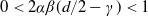 $0<2\alpha \beta (d/2-\gamma )<1$ if
  $m=1,$ and for
 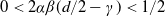 $0<2\alpha \beta (d/2-\gamma )<1/2$ if
  $m=2.$
Proof. The proof follows straightforwardly from Equations (48) and (49). Specifically, for  $m=1,$
 \begin{align}\sigma_{1,\mathcal{K}}^{2}(T)&=2T^{2}|\mathcal{K}|^{2}\int_{[0,1]}(1-\tau)\int_{0}^{\mathcal{D}(\mathcal{K})}C_{Z}(z ,T\tau )\psi_{\rho_{\mathcal{K}}}(z)dzd\tau\nonumber\\
&=2T^{2}|\mathcal{K}|^{2}\int_{[0,1]}(1-\tau)\int_{0}^{\mathcal{D}(\mathcal{K})}\frac{1}{(a[T\tau]^{2\alpha }+1)^{\beta d/2}}\nonumber\\
&\qquad \times E_{\nu }\!\left( -\frac{z ^{2\gamma }}{(a [T\tau ] ^{2\alpha }+1)^{\beta \gamma }}\right)\psi_{\rho_{\mathcal{K}}}(z)dzd\tau\nonumber\\
&\geq 2T^{2}|\mathcal{K}|^{2}\int_{[0,1]}(1-\tau)\int_{0}^{\mathcal{D}(\mathcal{K})}\frac{1}{(a[T\tau]^{2\alpha }+1)^{\beta d/2}}\nonumber\\
&\qquad\qquad\qquad\qquad \times\frac{1}{\left[ 1+\Gamma (1-\nu)\frac{z^{2\gamma }}{\left[1+aT^{2\alpha}\tau ^{2\alpha}\right]^{\beta \gamma}}\right]}\psi_{\rho_{\mathcal{K}}}(z)dzd\tau\nonumber\end{align}
\begin{align}\sigma_{1,\mathcal{K}}^{2}(T)&=2T^{2}|\mathcal{K}|^{2}\int_{[0,1]}(1-\tau)\int_{0}^{\mathcal{D}(\mathcal{K})}C_{Z}(z ,T\tau )\psi_{\rho_{\mathcal{K}}}(z)dzd\tau\nonumber\\
&=2T^{2}|\mathcal{K}|^{2}\int_{[0,1]}(1-\tau)\int_{0}^{\mathcal{D}(\mathcal{K})}\frac{1}{(a[T\tau]^{2\alpha }+1)^{\beta d/2}}\nonumber\\
&\qquad \times E_{\nu }\!\left( -\frac{z ^{2\gamma }}{(a [T\tau ] ^{2\alpha }+1)^{\beta \gamma }}\right)\psi_{\rho_{\mathcal{K}}}(z)dzd\tau\nonumber\\
&\geq 2T^{2}|\mathcal{K}|^{2}\int_{[0,1]}(1-\tau)\int_{0}^{\mathcal{D}(\mathcal{K})}\frac{1}{(a[T\tau]^{2\alpha }+1)^{\beta d/2}}\nonumber\\
&\qquad\qquad\qquad\qquad \times\frac{1}{\left[ 1+\Gamma (1-\nu)\frac{z^{2\gamma }}{\left[1+aT^{2\alpha}\tau ^{2\alpha}\right]^{\beta \gamma}}\right]}\psi_{\rho_{\mathcal{K}}}(z)dzd\tau\nonumber\end{align}
 \begin{align}
&\geq 2T^{2}|\mathcal{K}|^{2}\int_{[0,1]}(1-\tau)\int_{0}^{\mathcal{D}(\mathcal{K})}\frac{1}{(a[T\tau]^{2\alpha }+1)^{\beta d/2}}\nonumber\\
&\qquad\qquad\qquad\qquad\times\frac{a^{\beta\gamma}T^{2\alpha \beta \gamma }\tau^{2\alpha \beta \gamma } }{\left[ \left[1+aT^{2\alpha}\tau ^{2\alpha}\right]^{\beta \gamma}+\Gamma (1-\nu)z^{2\gamma }\right]}\psi_{\rho_{\mathcal{K}}}(z)dzd\tau\nonumber\\
&=2T^{2\!\left(1-\alpha \beta \!\left(\frac{d}{2}-\gamma \right)\right)}|\mathcal{K}|^{2}\int_{[0,1]}(1-\tau)\int_{0}^{\mathcal{D}(\mathcal{K})}\frac{1}{\left(a\tau^{2\alpha }+\frac{1}{T^{2\alpha}}\right)^{\beta d/2}}\nonumber\\
&\qquad\qquad\qquad\qquad \times\frac{a^{\beta\gamma}\tau^{2\alpha \beta \gamma } }{\left[ \left[1+aT^{2\alpha}\tau ^{2\alpha}\right]^{\beta \gamma}+\Gamma (1-\nu)z^{2\gamma }\right]}\psi_{\rho_{\mathcal{K}}}(z)dzd\tau.\nonumber\\
\end{align}
\begin{align}
&\geq 2T^{2}|\mathcal{K}|^{2}\int_{[0,1]}(1-\tau)\int_{0}^{\mathcal{D}(\mathcal{K})}\frac{1}{(a[T\tau]^{2\alpha }+1)^{\beta d/2}}\nonumber\\
&\qquad\qquad\qquad\qquad\times\frac{a^{\beta\gamma}T^{2\alpha \beta \gamma }\tau^{2\alpha \beta \gamma } }{\left[ \left[1+aT^{2\alpha}\tau ^{2\alpha}\right]^{\beta \gamma}+\Gamma (1-\nu)z^{2\gamma }\right]}\psi_{\rho_{\mathcal{K}}}(z)dzd\tau\nonumber\\
&=2T^{2\!\left(1-\alpha \beta \!\left(\frac{d}{2}-\gamma \right)\right)}|\mathcal{K}|^{2}\int_{[0,1]}(1-\tau)\int_{0}^{\mathcal{D}(\mathcal{K})}\frac{1}{\left(a\tau^{2\alpha }+\frac{1}{T^{2\alpha}}\right)^{\beta d/2}}\nonumber\\
&\qquad\qquad\qquad\qquad \times\frac{a^{\beta\gamma}\tau^{2\alpha \beta \gamma } }{\left[ \left[1+aT^{2\alpha}\tau ^{2\alpha}\right]^{\beta \gamma}+\Gamma (1-\nu)z^{2\gamma }\right]}\psi_{\rho_{\mathcal{K}}}(z)dzd\tau.\nonumber\\
\end{align}
From (50), Condition 2(ii) holds for 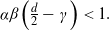 $\alpha \beta \!\left(\frac{d}{2}-\gamma \right) <1.$
In a similar way to (50), it can be proved that for  $m=2,$ Condition 2(ii) holds for
 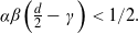 $\alpha \beta \!\left(\frac{d}{2}-\gamma \right)<1/2.$
As a direct consequence of Proposition 2, we obtain that Theorems 2 and 3 hold for the family of spatiotemporal Gaussian random fields with covariance function (49).
Similar assertions hold for the family of spatiotemporal covariance functions
 \begin{align}
&\widetilde{C}_{Z}(\mathbf{z},\tau )=\frac{\sigma ^{2}}{[\psi (\tau ^{2})]^{d/2}}\varphi \!\left( \frac{\left\Vert \mathbf{z}\right\Vert ^{2}}{\psi (\tau ^{2})}\right),\qquad \sigma ^{2}\geq 0,\ (\mathbf{z},\tau )\in \mathbb{R}^{d}\times \mathbb{R}, \nonumber\\
&\varphi (u)=\frac{1}{(1+cu^{\gamma })^{\nu }},\qquad u\geq 0,\ c>0, \ 0<\gamma \leq 1, \ \nu >0,\nonumber\\
\psi (u)& = (1+au^{\alpha })^{\beta },\qquad a>0,\ 0<\alpha \leq 1,\ 0<\beta \leq 1,\ u\geq 0,\end{align}
\begin{align}
&\widetilde{C}_{Z}(\mathbf{z},\tau )=\frac{\sigma ^{2}}{[\psi (\tau ^{2})]^{d/2}}\varphi \!\left( \frac{\left\Vert \mathbf{z}\right\Vert ^{2}}{\psi (\tau ^{2})}\right),\qquad \sigma ^{2}\geq 0,\ (\mathbf{z},\tau )\in \mathbb{R}^{d}\times \mathbb{R}, \nonumber\\
&\varphi (u)=\frac{1}{(1+cu^{\gamma })^{\nu }},\qquad u\geq 0,\ c>0, \ 0<\gamma \leq 1, \ \nu >0,\nonumber\\
\psi (u)& = (1+au^{\alpha })^{\beta },\qquad a>0,\ 0<\alpha \leq 1,\ 0<\beta \leq 1,\ u\geq 0,\end{align}
for  $\alpha \beta \!\left(\frac{d}{2}-\gamma \nu \right) <1$ if
  $m=1,$ and for
  $\alpha \beta \!\left(\frac{d}{2}-\gamma \nu \right)<1/2$ if
  $m=2.$
6. Discussion
As mentioned in the introduction, the main contribution of this paper relies on deriving a general reduction principle in Theorem 1, beyond the regularly varying condition on the spatiotemporal covariance function of the underlying Gaussian random field. Hence, we can analyze a larger class of spatiotemporal covariance functions. In particular, we consider some examples of the Gneiting class of covariance functions (see Gneiting [Reference Gneiting13]), which is popular in many applications, including in meteorology and earth sciences.
By considering homogeneous and isotropic Gaussian random fields restricted to a spatial convex compact set evolving over time, this paper applies an extrinsic random field approach, in contrast to the intrinsic spherical one adopted in Marinucci, Rossi and Vidotto [Reference Marinucci, Rossi and Vidotto32]. Thus, the isonormal representation of the underlying spatiotemporal Gaussian random field on  $\mathbb{R}^{d}\times \mathbb{R},$ and the characteristic function of the uniform probability distribution on a temporal interval and a spatial convex compact set, allow us to adopt a continuous spectral-based approach to derive the limit results in our framework (see, e.g., Proposition 1).
A time-varying pure point spectral approach is considered in Marinucci, Rossi and Vidotto [Reference Marinucci, Rossi and Vidotto32], based on projection onto the orthonormal basis of spherical harmonics. Different ranges of dependence are then assumed at different spatial resolution levels in the sphere. In our paper, under the temporal decay velocity of the space–time covariance function established in Condition 2, a general reduction principle is derived in Theorem 1, providing the limiting distribution of properly normalized integrals of nonlinear transformations of spatiotemporal Gaussian random fields. Theorem 2 constitutes a particular case of Theorem 1, where the scaling also depends on the threshold u, which provides a scenario similar to that of Theorem 1 in Marinucci, Rossi and Vidotto [Reference Marinucci, Rossi and Vidotto32], when the zeroth-order multipole component is long-memory, and all the other multipoles have asymptotically smaller variance.
Note also that Proposition 2 of this paper corresponds to the separable case in time and space, which presents a different situation from the nonseparable case addressed in Marinucci, Rossi and Vidotto [Reference Marinucci, Rossi and Vidotto32]. Furthermore, Marinucci, Rossi and Vidotto [Reference Marinucci, Rossi and Vidotto32] consider different orthonormal bases for space and time, in terms of the spherical harmonics and complex exponentials, respectively. These bases do not provide a diagonal spectral representation of the space–time covariance function of the underlying Gaussian random field. The composite Rosenblatt distribution then arises from the set of multipoles where the larger dependence range (long memory) is displayed (as in the reduction theorems). This non-diagonal representation induces a similar effect to considering Hermite rank  $m=2,$ in the case of separable covariance functions in space and time, admitting a diagonal representation in terms of the complex exponentials in space and time (see Proposition 1).
As a subsequent paper will show, our results can be extended to the nonseparable case, in terms of a bounded spatially varying long-memory parameter satisfying Condition 2(ii). This could be the case, for example, of an extended version of Proposition 1, in terms of nonseparable covariance functions, involving a parameter  $\alpha ({\cdot})$ that is bounded across all spatial frequencies. In that case, when the supremum of
  $\alpha ({\cdot})$ over the spatial frequencies satisfies Condition 2(ii), Theorem 1 holds under Condition 2(i).
Funding information
This work has been supported in part by the projects MCIN/AEI/PGC2018-099549-B-I00, CEX2020-001105-M MCIN/AEI/10.13039/501100011033, and by the grant A-FQM-345-UGR18, cofinanced by ERDF Operational Programme 2014–2020 and the Economy and Knowledge Council of the Regional Government of Andalusia, Spain. N. Leonenko was partially supported by LMS grant 42997, and ARC grant DP220101680. N. Leonenko and M. D. Ruiz-Medina were supported by the Isaac Newton Institute (Cambridge) program Fractional Differential Equations.
Competing interests
There were no competing interests to declare which arose during the preparation or publication process for this article.


