3D datasets

A data cube refers to any 3D (or higher) array of values—such as a stack of 2D black-and-white images representing a spatial volume. Unlike crystallographic and surface data, data cubes grow rapidly—a 1024 × 1024 × 1024 data cube of 32-bit values occupies 4.29 gigabytes of memory. Each 3D element in the data cube is termed a voxel, analogous to a pixel in a 2D image. In tomography, each voxel in a data cube contains a value that represents intensity at a point (x,y,z) in the volume, which may relate to the composition or some other characteristic of the object at that point. For example, in medical X-ray computed tomography (CT), higher intensity represents denser material; a human head has brighter values at points where the hard skull is located than where soft brain matter is located [Reference Hounsfield1,Reference Phillips and Lannutti8]. In nanoscale STEM tomography, high-Z gold nanoparticles appear brighter than low-Z silica nanoparticles [Reference Weyland4]. Because intensity values are provided at all voxels, not just at material surfaces, tomography reveals the entire 3D internal structure of an object [Reference Hounsfield1].

3D data cubes are not limited to spatial volumes. In a hyperspectral map the third dimension is spectroscopic (x-y-wavelength, or x-y-energy) [Reference Cueva9]. In a black-and-white movie, the third dimension is time (x-y-time). In a tomographic tilt series, the data cube contains images at different projection angles (x-y-angle). Although tomographic volume data is the most directly interpretable, tomviz is capable of visualizing any type of 3D data cube.

Loading volumetric data into tomviz

In tomviz, users can load a variety of datatypes stored as a TIFF, PNG, raw binary data, MRC, or HDF5 under “File > Open” in the top menubar. For convenience, tomviz comes packaged with an example dataset, a “Star Nanoparticle (Reconstruction),” so users can immediately explore different visualization techniques. The dataset contains the 3D structure of a Co₂P hyperbranched nanoparticle; it can be opened from the menubar under “Sample Data.” For further exploration of visualization techniques, five high-quality electron tomography datasets from the peer-reviewed literature have been made publicly available for researchers to use (Levin et. al., 2016). The datasets can be accessed under “Sample Datasets > Download More Datasets,” or they can be downloaded at https://dx.doi.org/10.6084/m9.figshare.c.2185342.

The tomviz user interface

New visualizations can be added from the Visualization menu or by clicking an icon from the Toolbar:

All tomviz visualizations are interactive 3D objects that can be rotated by clicking and dragging in the render window(s). The dataset and its associated visualizations—an outline, a volume, and a slice in the case of Figure 1—are listed in the upper left-hand Pipelines (Figure 1a). As the user adds new visualization modules to a dataset, these will be displayed in the pipeline for that dataset. Each dataset that is opened in tomviz is assigned its own pipeline. This allows the user to easily keep track of all changes made to every dataset. Further properties for each selected visualization module or dataset are shown in the lower left-hand Properties Panel (Figure 1b).

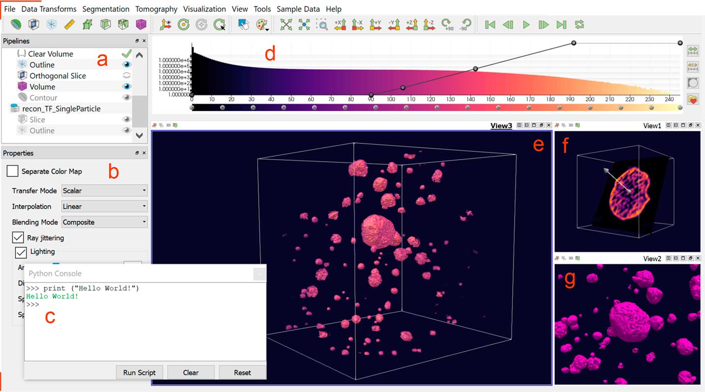
Figure 1 The tomviz graphical user interface for 3D visualization of tomographic data. Once a dataset has been loaded, the data pipeline is populated (a). A variety of visualization types are available to be used in combination for analysis—with parameters specified in the module properties panel (b). A Python interface offers advanced scientific processing of data (c). A histogram of voxel intensities is displayed top center (d). The line across the histogram represents the opacity map and can be altered interactively. Here a reconstruction of porous PtCu nanoparticles is visualized using a volume render (e), a non-orthogonal slice through one particle (f), and a contour surface (g). Tabs, and divisions within a tab, allow multiple simultaneous renderings and camera angles.

In addition to a suite of visualization tools—the subject of this tutorial—3D data processing is also integrated into the tomviz user interface. A Python console (Figure 1c) can be opened from “Tools > Python” Console under the top menubar. Users can execute pre-written python scripts or create their own code using numpy, scipy, or ITK. The Data Transform and Tomography menus contain pre-written algorithms for image processing, alignment, and tomographic reconstruction of raw electron microscopy data. After these scripts are executed in Python, they are sent back to tomviz for immediate visualization. Data transforms appear in the pipeline in the order in which they are executed. Double-clicking on a transform listed in the pipeline opens a new window displaying the Python code used to implement the transformation, which the user may edit if desired. The tomviz pipeline uniquely preserves all steps for reproducible workflow.

After a dataset is loaded, a histogram panel appears (Figure 1d). Colors in the histogram represent a colormap that quantitatively correlates colors in a visualization to corresponding dataset values. This color map corresponds only to the dataset currently selected under Pipelines. Different color maps can be chosen from a list of presets, or the map may be adjusted interactively by clicking and dragging points on the color bar underneath the histogram.

By default, tomviz automatically adds a box outline and an orthogonal slice taken through the volume center in a Render View panel. Users may then add new visualizations of their own to the default Render View panel (Figure 1e). Additional Render View panels can be added from the Toolbar: , allowing multiple visualizations to be shown simultaneously in separate panels, at different viewing angles (Figure 1f, Figure 1g).

I. Slicing data with planes

The simplest method for detailed examination of specific features of the internal 3D structure of an object is to inspect individual 2D sections—or slices—through the 3D dataset. The tomviz package features two different slice viewing tools. Orthogonal slicing allows users to view slices through the data perpendicular to one of the principal x, y, or z axes. Both the plane (x, y, or z), and the position of the slice can be altered interactively in the Properties panel (Figure 1b), as can the opacity/transparency of the slice. An example of orthogonal slicing is shown in Figure 2. In this figure, an orthogonal slice is extracted from the center of a reconstruction of platinum nanoparticles on a carbon nanofiber support. Platinum nanoparticles can be seen on both the interior and exterior surfaces of the nanofiber in this slice.

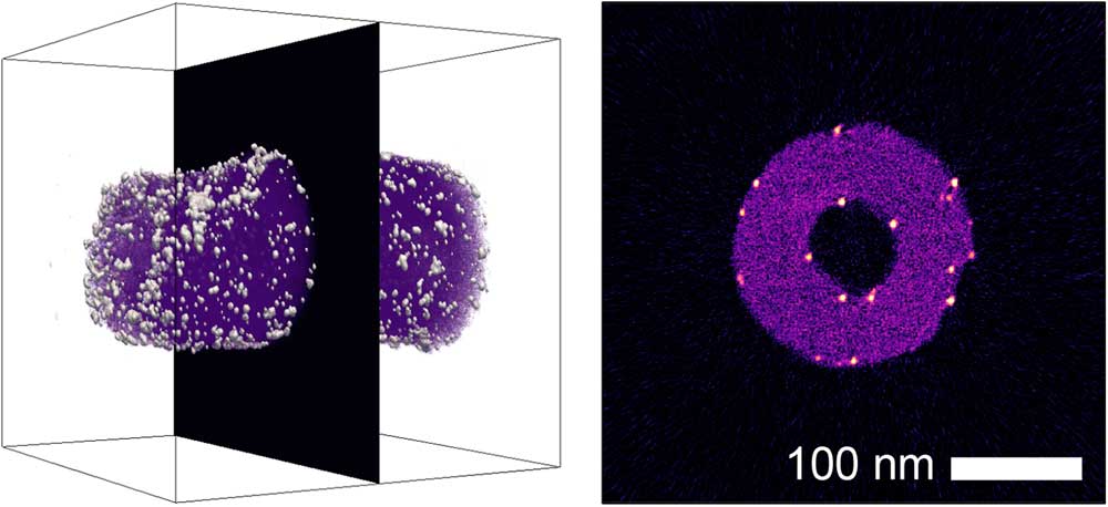
Figure 2 A volumetric reconstruction of platinum nanoparticles on a carbon nanofiber [Reference Levin10], showing the position of an extracted orthogonal slice. In the extracted slice, platinum nanoparticles (white/orange) can be identified on both the interior and exterior surfaces of the nanofiber (magenta).

Non-orthogonal slicing offers greater flexibility, allowing users to view slices through the reconstruction at any orientation. The orientation and position of a non-orthogonal slice can be adjusted interactively by clicking and dragging the axis and slice in the Render View panel (Figure 1f) or manually by entering values in the Properties panel (Figure 1b).

II. Surface rendering

Surface rendering was originally applied to volumetric data to offer a more direct method of visualizing the 3D morphology of structures than 2D slices [Reference Lorenson and Cline11]. In surface rendering, a surface contour of constant intensity is generated from a user-specified intensity value using a fast-flying edges algorithm [Reference Schroeder12]. In tomviz, the intensity value of the surface contour can be entered manually or adjusted using a slider in the Properties panel (Figure 1b). The color, opacity/transparency, and lighting (specularity) of a surface render can also be altered in the Properties panel. Surfaces are rendered in a single color. By default, this color will change as the intensity of the surface is changed, following the color map. Alternatively, the user can choose to use a fixed color for all surfaces. Figure 3 shows different isosurfaces of a porous PtCu nanoparticle with a fixed color, and different combinations of intensity and opacity. At full opacity, only the exterior of a surface can be visualized. Reducing the opacity of a surface contour allows the surface of interior structures, such as pores, to be visualized.

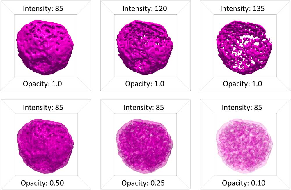
Figure 3 Surface renderings of a porous PtCu nanoparticle [Reference Levin10] at different values of intensity and surface opacity. At full opacity, only the exterior of a surface contour is visible. At low intensity, this exterior surface contour corresponds to the exterior surface of the nanoparticle. As the intensity of a surface contour is increased, features of the interior of the particle become visible. Varying the opacity at lower intensity allows the user to see through the exterior surface and observe the interior surfaces of the nebulous internal pore structure of the particle.

III. Volume rendering

Volume rendering was originally developed to visualize more complex 3D structures with many gray values, which are difficult to visualize by surface rendering [Reference Kaufman13]. In volume rendering, each voxel is assigned both a color and an opacity based on its intensity. The gray line overlaying the histogram of the data in the tomviz interface (Figure 1d) is the opacity map of the visualization, and together with the color map, this defines the color-opacity map. Figure 4 shows example volume renderings of a Co₂P star-shaped nanoparticle at different viewing angles, with their associated color-opacity maps. In tomviz, the color-opacity map can be adjusted interactively with dynamically updated 3D visualizations. The user may simply click and drag a point on the gray line overlaying the histogram to vary the opacity of different voxels in the volume render. In the examples shown in Figure 4, the color-opacity map has been set so that the opacity increases with increasing voxel intensity, and the color becomes increasingly light with increasing voxel intensity. The range of the color map has been adjusted to enhance the brightness and contrast of the visualization. Minor adjustments to the color-opacity map can have a noticeable influence on the final appearance of the visualization of an object. It is essential for users to adjust the color-opacity map to produce a volumetric visualization that reflects the features of the sample that they have imaged. In addition, it is important to include the color-opacity map with any published scientific volumetric renderings to aid interpretation.

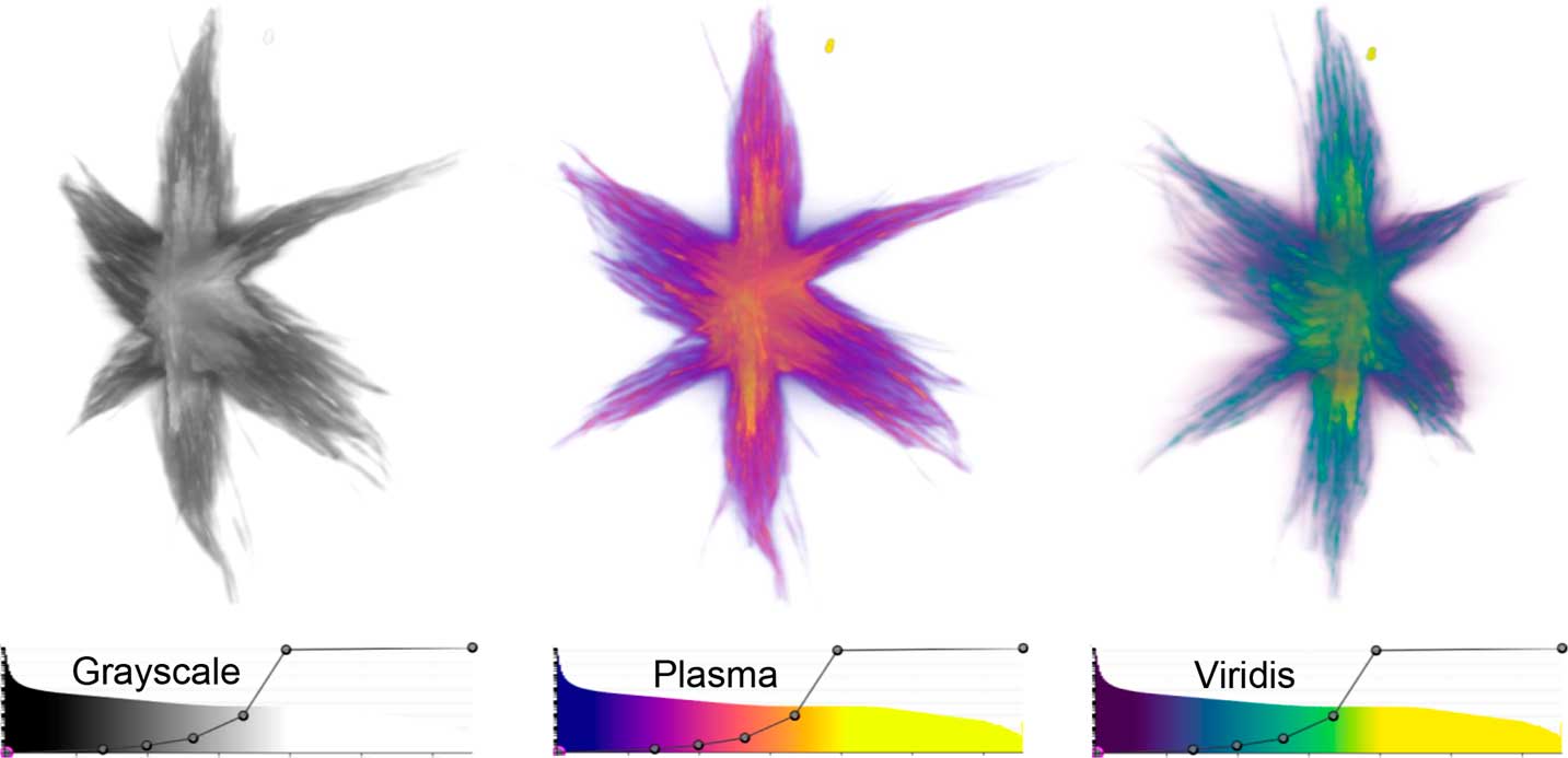
Figure 4 Volume renderings of a Co₂P nanoparticle [Reference Levin10] viewed from different perspectives using Grayscale, Plasma, and Viridis color-opacity maps. In these renderings, the dense internal core of the nanoparticle is displayed in lighter, more opaque colors, whilst the branches that protrude from the core are displayed as darker and more transparent colors. The color-opacity maps used in the visualizations are shown below each view of the particle.

Bounding boxes and scale

A bounding box frame outlines the edges of a dataset, giving the viewer an impression of 3D depth perception with a non-orthogonal perspective on a 2D screen. In the same way that a parallel set of train tracks converges into the distance in the real world, so do most 3D visualizations—features in the foreground appear larger. A bounding box adds more than aesthetic appeal because it helps restore the interpretability of a 3D structure rendered on a 2D screen. Most of all, a bounding box allows scientists to put meaningful scale bars along an edge. In tomviz, voxel distances can be displayed by selecting “View > Show Axis Grid.” An example visualization with dimensional scales is shown in Figure 5.

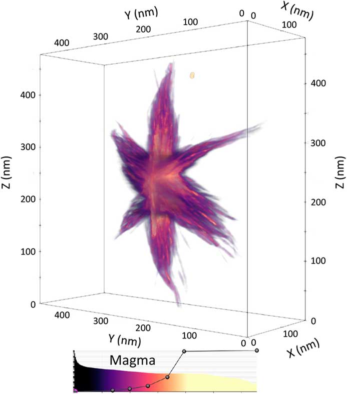
Figure 5 Volume rendering of the Co₂P nanoparticle from Figure 4, enclosed in a bounding box with scale markers in nanometers shown on each axis of the box. Using perspective, the bounding box and scale together convey a sense of the 3D size of the particle. The color-opacity map of the volume render is shown underneath the visualization.

Animation

In addition to 2D figures, an animation of a 3D visualization is an effective method of illustrating the 3D structure of an object. In tomviz, an animation tool allows users to produce simple animations, such as a 360^o orbit around a 3D object, or more complex animations by moving the viewing angle between a series of user-specified positions. A still from an animation is shown in Figure 6. The full animation is available online in the digital edition of this issue at this web address: https://doi.org/10.1017/S1551929517001213. This animation shows a mixed volume and surface rendering of platinum nanoparticles decorating a carbon nanofiber of ~170 nm in diameter. The carbon fiber is visualized in black using a volume render, with the color-opacity map set such that only voxels with an intensity corresponding to the carbon fiber are visible. The platinum nanoparticles are visualized using a turquoise surface contour, with the intensity of the contour set such that only platinum is visible.

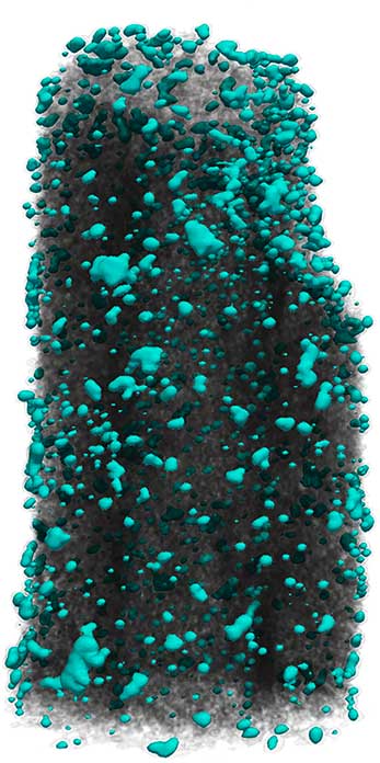
Figure 6 Still image from an animation of platinum particles (turquoise color) on a carbon fiber. The animation is available online in the digital edition of this issue at this web address: https://doi.org/10.1017/S1551929517001213.

Save and share

Whilst a high-quality manuscript figure can convey a sense of 3D structure, it is no substitute for interactive visualization and exploration of a volumetric dataset. With tomviz, the data, visualization pipeline, and software can all be shared with other scientists. Simply click “File > Save State” to share the tomviz state file (*.tvsm) and volumetric data with colleagues. For scientific publication, a screenshot of the visualization can be exported using the existing background or a transparent background by executing “File > Save Screenshot.”

Open-source license

Tomviz is made freely and publicly available as open-source software under the 3-clause BSD License that enables any party to copy, distribute, and make modifications to the software. This includes government organizations, for-profit and not-for-profit educational institutions, and commercial organizations, as well as individuals. Tomviz is hosted on Github and is open to further contributions from new users.