Introduction

Because of its structure (Reference WeeksWeeks, 1962; Reference Weeks and AssurWeeks and Assur, 1964; Reference Hoekstra, Hoekstra, Osterkamp and WeeksHoekstra and others, 1965; Reference Lofgren and WeeksLofgren and Weeks, 1969), sea ice is a non-homogeneous material and its optical properties are correspondingly complex. In the work to be described here, the purpose was to focus upon the optical extinction coefficient and its variation with the wavelength of the radiation and the salinity of the ice. As used here, “extinction” refers to the total amount of intensity removed from a collimated, monochromatic light source by the mechanisms of scattering plus absorption. This convention is not always followed and so it is important not to confuse the measurements reported below with measurements of scattering or absorption alone.

Another source of possible confusion is that arising from the basic character of the measurements, It has been shown (Reference Little, Little, Allen and WrightLittle and others, 1972) that the attenuation of sunlight by sea ice in situ is orders of magnitude different from the. attenuation of a collimated light beam by a sample of the same sea ice removed to the laboratory. This is principally because the environment of the sample in situ provides for additional light to be scattered from adjacent sections of the ice sheet since the entire sheet is illuminated and sea ice is a turbid medium. In effect the in situ measurements are representative of the ice sheet and its environment rather than specifically of sea ice as a material.

The extinction coefficient is not measured directly. The transmission Y is measured and, by definition of the extinction coefficient k_e,

(1)

where z is the thickness of the sample traversed by the radiation. In general, k_e is a function of wavelength, temperature, and the characteristics of the sample. In the case of sea ice, the characteristics that immediately suggest themselves are the salinity of the ice and its structural properties such as grain size and grain orientation. Since the history of the specimen is known to influence all of these properties, it can be expected that the history of the specimen will influence k_e . The work reported below was done for a specific specimen history and a specific temperature so that it would be possible to examine the effects of wavelength and salinity separately. While the control of its history probably worked to provide limitations on grain size and grain orientation, no direct control or measurement of either was attempted. The consequences of this will be discussed.

Reference Davis and MunisDavis and Munis (1973) investigated the dependence of k_e upon the salinity profile of NaCl-ice grown under conditions designed to simulate the natural environment of sea ice. They suggested that, at a given optical wavelength and for temperatures above the eutectic point, it might be possible to represent the variation of k_e with salinity by an empirical relation of the form

(2)

where x is the salinity of the ice and A, B, and C are parameters dependent upon the history of the ice, wavelength, and temperature. Their range of salinities was severely limited and so they were not able to determine an adequate set of parameters (A, B, C). The physical implications of such a relationship will be discussed here and the data described above will be used to test Equation (2) for a specific wavelength, specimen history, and temperature.

Experimental Procedure

The temperature chosen for all experiments was —20° C, a temperature just above the eutectic point for NaCl-ice.

The specimen history was in part dictated by the requirements of the optical systems. It was necessary to devise a method of preparing specimens that were uniform in thickness and which bad parallel, undeformed surfaces. Also, provisions for mounting such specimens in the optical systems had to be considered. To do this, a device to be called a ’ sea-ice rack ’ or “SIR” was designed.

Figure 1 is a diagram of a SIR. It has five major parts—a rack made of bakélite, two rubber gaskets, and two aluminum gaskets. These five parts are secured by 36 screws. The rack contains ten cylindrical holes and the screws are arrayed about these holes so as to secure the two sets of gaskets to either side of the rack in a way that makes the SIR watertight. The cylindrical holes were most often filled with a solution of NaCl and water adjusted to a given salinity and, in a few cases, with natural sea-water of a known salinity. The level of filling was adjusted so that the expansion during freezing was exactly accommodated by elastic deformation of the rubber gaskets, leaving the ice exactly the thickness of the rack— 1.27 cm— and the surfaces free of deformities. After the SIR had been left in an ambient atmosphere of —20° C for a period of 24 h, its gaskets were removed and the specimens examined for defects.

Fig. 1. Schematic diagram of a sea-ice rack. A is an Al gasket drilled with 18 holes to accept 18 flat-headed screws. B is a rubber gasket drilled with 18 holes to mate, with A. C is a bakélite rack drilled and topped on top and bottom sides to accept 18 screws on each face. E is a typical flat-headed screw used to secure the gaskets to the rack. F is a cylindrical hole extending through the. thickness of the rack. D gives the diameter of the two sizes o i cylindrical holes.

After visual examination, the specimens were left in the rack and this was inserted into a permanent mount on the optical bench. The configuration of the optical bench is shown in figure 2. A collimated beam of light of a wavelength, 6 328 Â, was generated by a Perkin-Elmer Model 5200 cw He—Ne laser. This beam was modulated with a chopper operated at 400 Hz, passed through the sample, and detected by the circuit shown in Figure 2. The intensity of the beam passing through an empty cylinder of the rack was used as a reference.

When transmission measurements had been completed, the rack was removed from the cold room in which the specimens had been prepared and observed. The specimens were allowed to melt and the salinity of the melt water was measured in order to determine the actual salinity of the ice.

A Perkin-Elmer Model E-14 spectrophotometer was used to measure transmission at wavelengths other than 6 328 Â. For these measurements, the spectrophotometer was modified to accept the rack of the SIR. Two different salinities—5.5 and 35.9 g/kg—were studied over the wavelength range from 4 000 to 8 000 Â. The accuracy of the transmission measurements in this system declined at each end of the selected range due to the limitations of the spectrophotometer.

In selected cases, measurements of the temperature gradients during freezing were made, and it was found that freezing proceeded from the top and bottom toward the center of each cylindrical specimen. This had the effect of driving the air bubbles and brine toward the center of the samples. Since the sample size was deliberately taken to be small (see the dimensions shown in Figure 1), the effects on transmission of any temperature or salinity gradients were minimized. After the 24 h freezing period, it was found that no temperature gradient in excess of 0.2 deg/cm existed either in the ice or between the ice and the ambient temperature.

All of the reported transmission measurements were made with the top face (of the specimens as frozen) placed toward the light source. Measurements were also taken with the bottom face toward the light source, and it was found that there was no significant difference between these and those for the other configuration.

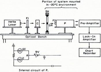
Fig. 2. Optical bench configuration and detector circuit. F₁ is a neutral density filter. C is a 400 Hz chopper. SH is the specimen holder designed to mount the SIRs. SIR is a sea-ice rack mounted so that the beam passes through a sample. F2 is a line transmission filter. P is a silicon diffused-pin photo-diode positioned 1 cm from the back face of the sample. It has a window of 1.6 cm diameter. The internal circuit of P and associated elements is shown along with the amplification and recording system. Part of the system was mounted in the cold room where the samples were prepared. The cold-sensitive components were mounted in an adjacent warm room kept at room temperature.

Results

The data obtained with the laser system are shown in Figure 3. Here, transmission if plotted versus salinity. The absolute uncertainties in the transmission and salinity measurements were determined to be, respectively, 26% and 5%. These data show the variation o-transmission (through 1.27 cm of NaCl-ice) with salinity for a temperature of — 20° C, a wavelength of 6 328 Â, and the specimen history detailed above. The shaded portion gives the limits of the scatter in the data. The error bars depict the standard deviation about the mean for the transmission at a given salinity. Since a SIR holds ten specimens, it is possible to consider each specimen as a separate piece of data when computing the standard deviation. This was not done. Since all of the specimens in a single SIR batch were made under the same conditions, the average of their transmissions was considered as a single piece of data. Although the conditions were duplicated in so far as possible when preparing a new SIR batch for the same salinity, it was felt that the individual specimens in a single batch could be expected to be more alike than specimens from different batches. Therefore each point on the graph in Figure 3 represents an average of from 6 to 14 batch averages, depending upon the number of batches made at each salinity. In general, it was more difficult to prepare specimens at lower salinities because of the increase in expansion during freezing. The greater expansion pressures were difficult to accommodate so that the surfaces of the samples were not distorted. For this reason, fewer batches were obtained at the lower salinities and the corresponding standard deviations are therefore larger.

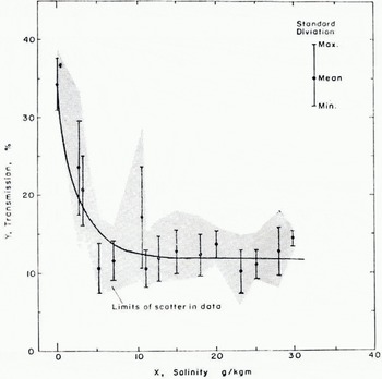
Fig. 3. Relationship between transmission Y and salinity X of salt-ice. The solid curve represents the empirical relationship. The dots represent actual data as described by the insert. The shaded area represents the limits of scatter of all the data.

The scatter averages 67% and cannot be explained by the absolute uncertainties of the measurements themselves. The possible reasons for this result will be discussed in the next section. The standard deviations average 22% and are within the experimental uncertainties. The salient characteristics of the data may be summarized in three statements: (1) The transmission of pure ice frozen in the same manner is substantially larger than that of NaCl-ice. (2) A small increase in salinity is accompanied by a rapid decrease in transmission. (3) After a salinity of 10 g/kg is reached, further increase in the salinity has little effect upon the transmission. Any empirical relation that is to fit the data must display these characteristics. Furthermore, if the data are to be considered as reasonable, it should be possible to explain these characteristics in terms of the known character of Nacl-ice. The next section will be concerned with such a physical interpretation; the question of choosing an empirical relationship to fit the data will be discussed first.

The simplest approach would be to fit the data to two linear regression lines, one for the low-salinity data and one for the high-salinity data. From the point of view of physical interpretation, this is not as desirable as a smooth curve but, in view of the large uncertainties in the data, would be a reasonable approximation. This was not done because the empirical relationship (2) suggested by Davis and Munis (1973) appeared (o have a reasonable physical interpretation and to display the desired characteristics if the parameters (A, B, C) were such that

(3)

It was decided to fit the data to the empirical equation

(4)

which results from substitution of Equation (a) into Equalion (1). A least-squares fit of the data was performed using a Taylor series expansion. The resulting parameter set was

(5)

and the corresponding curve for Equation (4) is shown in Figure 3. An analysis of the fit showed that 95% of the data fit the curve within ±20%, which is within both the experimental uncertainty and the average of the standard deviations. Because the experimental uncertainty was large, this result does not establish the relationship given by Equation (4) as correct, but it does make it seem plausible.

The spectrophotometric data are shown in Figure 4. Some of the experimental difficulties involved in the measurement of the transmission were overcome by the configuration of this system and it was possible to reduce the experimental uncertainty in the transmission measurements to 10% in the central region of the wavelength range. The uncertainty in the wavelength measurements was less than 1%. Figure 4 shows a plot of transmission versus wavelength for two salinities -5.5 and 35.9 g/km. The temperature and specimen history was essentially the same as for the data obtained with the laser system. The error bars show the maximum scatter for each point. The points themselves were obtained from the average of the measurements of transmission for nine different samples of the same salinity at the same wavelength. It was found that there is no appreciable dependence of transmission on wavelength for the range 4 000 to 8 000 Â.

Fig. 4. Relationship between transmission Y and wavelength λ, for two mean values and salinities of salt-ice. The error bars represent the observed spread of transmission values for each wavelength sampled.

As explained in the description of experimental procedure, a few batches were made with sea-water. The sea-water was collected during the summer off the Maine coast. It had a salinity of 29±1 g/kg and the resulting ice samples had a salinity of 23±1 g/kg. The transmission characteristics of these samples was not appreciably different from that of NaCl-ice samples of the same salinity.

Discussion

Simple optical laws of geometrical optics (Reference Born and WolfBorn and Wolf, 1966, p. 39) cannot be applied to a turbid medium such as NaCl-ice. For a typical sample in these experiments, the optical depth was in the range 1 to 3 and so single-scattering theory (Van de Reference Van de HulstHulst, 1957, p. 6) also does not apply. The rigorous approach is a multiple-scattering theory such as that developed by Reference Mudgett and RichardsMudgett and Richards (1971). Such an approach is beyond the scope of this paper. Experimental work on the optical properties of pure ice (Reference Irvine and PollackIrvine and Pollack, 1968; Reference Bertie, Bertie, Labbé and WhalleyBertie and others, 1969; Schaef and Williams, 1973) indicate that, in the region 4000 to 8 000 Â of the electromagnetic spectrum, the absorption coefficient of pure ice is of the order of 10^-3 cm^-1 or smaller. Since salt-ice is known to be characterized by a pure-ice matrix interwoven with layers of brine inclusions, it is reasonable to suppose that scattering from brine, air bubbles, or other artifacts, makes the major contribution to the extinction observed in salt-ice. This suggests a simple model that can be used to display the essential physics of the optical behavior of salt-ice.

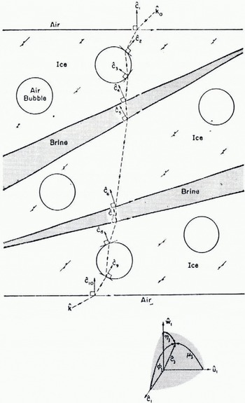
Fig. 5. Mosaic model of the layered structure typical of sea ice. The unshaded areas represent crystal grains of ice. The shaded areas represent brine pockets. The circles are air bubbles. The vectors, ĉ_j are the normals to the grain surfaces and are crystal directions m the respective grains except for ĉ₁, and ĉ₁₀. ĉ₁ and ĉ₁₀ are the normals to the faces of the sample and, depending upon how the sample was prepared, may or may not be crystal directions. In general, a given ĉ_j has a direction relative to ĉ₁ given by the angles, (φ, μ_j, η_j), between ĉ_j and each of the axes of the rectangular coordinate system (ĉ₁, û₁ ώ₁). For optical analysis, it is convenient to define û₁ as the normal to the plane of incidence of the incident beam of radiation. As depicted, the sample has randomly oriented grains. If a preferred orientation existed, and all of the interior grains would be aligned with each other but not necessarily with the faces of the sample. A sample path of a beam of radiation is traced through the sample. k₀ is the incident wave vector and k is the emergent wave vector.

The idealized model to be described is not to be interpreted as a rigorous representation of salt-ice structure. With this in mind, refer to Figure 5, which is a diagram of an idealized specimen of salt-ice. The specimen is considered to be a mosaic composed of perfect crystal grains of pure ice separated by extended grain boundaries containing concentrated salt solutions—the brine inclusions. Embedded in the crystal grains are air bubbles. The top and bottom surfaces are considered to be perfectly flat and parallel to each other. The interior surfaces, however, can be oriented at random with respect to the faces of the cylinder.

The beam of radiation strikes the top surface at an angle and, as it passes through the mosaic, it undergoes reflection and refraction at each of the surfaces it encounters. For simplicity, it is assumed that, once a portion of the intensity has been reflected back toward the source, it is lost to the transmitted beam, and that there is no appreciable loss of intensity due to absorption. As shown in Figure 5, the beam emerges from the bottom surface reduced in intensity and deviated in direction relative to its intensity and direction when it entered the mosaic. How much intensity is lost, or, equivalently, the transmission of the mosaic, would depend upon the number of surfaces encountered, the refractive indices of the various media— air, ice, and brine, and the orientations of those surfaces. Therefore, if real salt-ice bears a resemblance to the model, it could be expected that the orientations of its crystal grains, the configurations of its brine inclusions, and the distribution of air bubbles in its interior, would significantly influence extinction measurements such as those reported here.

How sensitive could the transmission be expected to be to a given preferred orientation of the crystal grains in a sample of salt-ice? It is impossible to give a quantitative answer to this question with the simple model shown in Figure 5. However, by assuming nominal values for the refractive indices, the grain size, and the bubble distribution, the qualitative behavior of the transmission as the orientation of the interior surfaces is changed can be determined for a mosaic of the order of the size of the samples studied in these experiments. The result is shown in Figure 6 for the nominal choice of 1.31 and 1.33 for the refractive indices of ice and brine, respectively, 0.1 cm for the grain size, and one air bubble per grain. The frame of reference shown in Figure 5 is that determined by the top surface and the plane of incidence of the beam as it enters the mosaic. The angle φ in Figure 6 is therefore the angle between the normals to the grain surfaces and the normal to the top surface, ĉ₁ For a preferred orientation of the grains, φ would be approximately the same for each grain, that is, the grain surfaces would be parallel to each other but inclined at an angle φ to the surfaces of the mosaic. From Figure 6, it can be inferred that a misorientation of a few degrees results in a large loss of transmission but an increase in the misorientation φ does not further affect the transmission until it nears a critical value associated with the critical angle for refraction from a medium to a less-dense medium (for example, from ice to air).

If the behaviour of the mosaic model is assumed to be representative of real salt-ice, then the three salient characteristics of the data that were listed in the previous section can be explained. Since the pure ice specimens were frozen under the same conditions as the salt-ice, they can be expected to contain air bubbles and grain boundaries but no brine inclusions. Therefore, since they have fewer internal interfaces to scatter intensity out of the beam, they exhibit a higher transmission than salt-ice. The transmission is below that of pure ice prepared in the form of a single crystal without air bubbles because these surfaces contribute to the extinction in the polycrystalline pure ice. The transmission drops dramatically upon the addition of small amounts of salt because any appreciable concentration of salt creates brine inclusions, which in turn add many additional scattering centers to the sample. Adding salt beyond a certain limit does not further lower the transmission because, at this point, no more brine inclusions are being created; the old ones are merely becoming larger, and it is the number of scattering surfaces rather than the actual size of the brine inclusions which is most important in removing intensity from the beam.

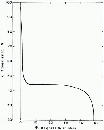
Fig. 6. Relationship between the transmission Y and the preferred orientation (φ. 90-φ) of the interior grains in the mosaic model of a sea-ice sample.

As noted previously, the observed scatter in the data was larger than expected. The mosaic model provides a clue as to the reason for this result. If indeed the orientation of the grains in salt-ice has an effect upon transmission similar to that displayed by the mosaic, then it can be expected that failure to control the grain orientations carefully, could result in a large scatter of data. In particular, suppose that a majority of the specimens examined in these experiments had grain orientations which fell in the “insensitive” range displayed in Figure 6. A few, however, had very small misorientations and others had very large misorientations. Most of the data would display a relationship between transmission and salinity in a regular fashion. The rest of it would display erratically high or low transmission and would substantially increase the average scatter of the data. This would suggest that grain orientation is at least as important a parameter as salinity in determining the optical properties of salt-ice.

Conclusions

The results obtained here indicate that, for optical wavelengths, there is no significant dependence of transmission through salt-ice on wavelength, a result that agrees with the known low value of the optical absorption coefficient for pure ice. This suggests that the major contribution to extinction in salt-ice is scattering from brine inclusions, grain boundaries, and air bubbles.

It was found that there is a significant dependence of transmission on the salinity of the ice but it was concluded that this effect is no more important (and may be less important) than the effect of grain orientations and grain size. Essentially, the introduction of any appreciable amount of salt into the ice lowers the transmission but the transmission reaches a saturation point where increasing the salinity of the ice has little effect upon transmission.

The relationship

(2)

proposed for extinction coefficient as a function of salinity has been examined and found to be plausible. However, any specimen history which caused the sample to drop to a temperature below its eutectic point and then to rise to a temperature above the eutectic point should be expected to display a much different relationship between transmission and salinity because of the structural changes introduced by crossing the eutectic point in this fashion, so any relationship between transmission and salinity must be given for a specific specimen history. If the values of the parameters (A, B, C) found from the data are substituted into Equation (2), the extinction coefficient values predicted are in the range 0.82 to 1.67 cm^-1 and this may be compared with the value of the extinction coefficients for sea ice cores quoted by Little and others (1972), which are in the range of 0.8 to 1.6 cm^-1.