


1. Introduction
In the classic Kelvin wave problem, one considers the production of waves in a uniform stream as flow passes a ship modelled as a point source at the origin. As shown by Kelvin (cf. Darrigol Reference Darrigol2005), the mathematical model can be posed in terms of Fourier integrals, after which an asymptotic analysis in the downstream limit predicts the well-known V-shaped wave pattern (see, e.g. Eggers Reference Eggers1992; Pethiyagoda, McCue & Moroney Reference Pethiyagoda, McCue and Moroney2014). In situations where the point source is submerged, the analysis is rendered more difficult (Lustri & Chapman Reference Lustri and Chapman2013), and this is a scenario we discuss in the article.
The Kelvin point-source model provides a geometrical linearisation of more complicated wave-generating bodies where the shape of the body may be assumed to be streamlined or thin (Tulin Reference Tulin2005). However, in situations of flows around blunt-bodied obstructions, the flow cannot be linearised about the uniform flow and we shall refer to such scenarios as involving a nonlinear geometry. As noted by Ogilvie (Reference Ogilvie1968), under such conditions, and it can be advantageous to develop asymptotics in the low-Froude or low-speed limit. This is characterised by small values of the Froude number,  $F$, defined via
 \begin{equation} \epsilon \equiv F^2 = \frac{U^2}{gL}, \end{equation}
which provides a measure of the relative balance between inertial forces, governed by the velocity and length scales,  $U$ and
  $L$, and gravitational forces, governed by
  $g$.
$g$.
Unfortunately, the study of the low-Froude limit,  $\epsilon \to 0$, presents notable challenges first remarked by Ogilvie (Reference Ogilvie1968), and now referred to as the ‘low-speed paradox’ (Tulin Reference Tulin2005). Specifically, suppose we write the velocity potential,
  $\phi$, as a series expansion in
  $\epsilon$:
 \begin{equation} \phi(x,y,z) = \phi_0(x,y,z) + \epsilon \phi_1(x,y,z) + \epsilon^2 \phi_2(x,y,z) +\cdots \end{equation}
The leading-order term,  $\phi _0$, corresponds to the so-called double-body flow where the free surface is flat. This term then encodes the information of the problem geometry; in our case this consists of uniform flow over a submerged point-source at
  $(0,0,-h)$:
 \begin{equation} \phi_0= \underbrace{Ux}_{Uniform\ flow} -\underbrace{\frac{\delta}{4{\rm \pi}} \left\{\frac{1}{\sqrt{x^2+y^2+(z-h)^2}}+\frac{1}{\sqrt{x^2+y^2+(z+h)^2}}\right\}}_{point\text{-}source\ terms}, \end{equation}
with  $\delta \ll 1$. The leading-order approximation,
  $\phi _0$, is wave-free, and as remarked by Ogilvie (Reference Ogilvie1968), the subsequent terms,
  $\phi _1$,
  $\phi _2$, etc., will also fail to capture wave phenomena. The waves are, in fact, exponentially small and beyond all orders of the expansion (1.2).
In fact, as a consequence of the singularly perturbed nature of  $\epsilon \to 0$, the base series in (1.2) diverges. The divergent expansion can be optimally truncated, and the exponentially small remainder sought. This yields
 \begin{equation} \phi(x,y,z)=\sum_{n=0}^{N}\epsilon^n\phi_n(x,y,z) + [A(x,y,z)\exp({-\chi(x,y,z)/\epsilon}) + \text{c.c.}]. \end{equation}
Here  $\chi$ is an important function known as the singulant. We will typically write the real-valued waves in complex-exponential form (c.c. denotes complex conjugate). Thus,
  $\operatorname {Re}\chi$ provides a measure of the exponential dependence of the waves and this is shown in figure 1. Exponential asymptotics provides the necessary tools for the determination of the beyond-all-orders contributions (Boyd Reference Boyd1999).

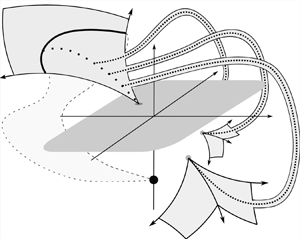
Figure 1. (a) A numerical surface wave calculated for  $\epsilon = 0.15$. The underlying steady flow is in the positive
  $x$-direction. A point-source (indicated by a bold circle) is placed below the free surface (indicated by light grey shading). The interaction of this flow with the point-source induces a downstream wavetrain. The free surface is calculated by direct numerical integration of the Fourier integral in Appendix A. (b) Schematic of the wavetrain; note that transverse and divergent waves form a wavetrain similar to, but distinct, from that seen in the classic Kelvin-ship problem.
There is a subtle aspect involving the exponentially small waves in (1.4). These waves do not exist at all points in  $\mathbb {R}^3$, but rather, they may switch on across certain critical manifolds known as Stokes surfaces. That is, in certain regions of the physical flow, the factor
  $A$ in (1.4) is identically zero, but
  $A$ becomes non-zero upon crossing a Stokes surface. This peculiar transition is known as the Stokes phenomenon, and is generic to many singularly perturbed problems.
For the above problem, the main Stokes surface corresponds to points,  $x, y, z\in \mathbb {C}$, that satisfy
  $\operatorname {Im}\chi = 0$ and
  $\operatorname {Re}\chi \geq 0$ (Dingle's criterion, cf. Dingle (Reference Dingle1973)). If one then obtains the intersection of the Stokes surface with real space, i.e.
  $x, y, z\in \mathbb {R}$, this manifold demarcates wave-free regions from regions with waves. Previously, in their analysis of the submerged Kelvin source problem, Lustri & Chapman (Reference Lustri and Chapman2013) derived analytical solutions to the Stokes surface intersection with the physical free surface, i.e. values of
  $\chi (x, y, z = 0)$. However, this seminal work hides two significant challenges to developing analogous techniques for problems with more challenging configurations: (i) it is not clear how
  $\chi$ can be obtained fully numerically; and (ii) it is not clear how to obtain values of
  $\chi$ off the free surface (i.e. determine the singulant everywhere). These two challenges form the main problems of this work.
In this article, we demonstrate a numerical methodology that allows Stokes surfaces to be derived for linear geometrical problems (such as the submerged point-source problem), but that can be generalised to nonlinear geometries, involving blunt-bodied obstructions (where  $\phi$ cannot be linearised about the uniform stream).
2. Background and open questions
The concepts of Stokes lines and Stokes surfaces are widely known in the analysis of differential equations, integral equations and, more generally, catastrophe theory (Wright Reference Wright1980; Berry & Howls Reference Berry and Howls1990). However, their application in problems of linear or nonlinear hydrodynamics is more recent. The study of water waves produced by flows past wave-generating bodies is extensive and we refer readers to the literature reviews found in Stoker (Reference Stoker1957), Wehausen & Laitone (Reference Wehausen and Laitone1960), Wehausen (Reference Wehausen1973) and Tulin (Reference Tulin2005).
Classically, Keller (Reference Keller1979) studied the Kelvin wave problem of a moving source on the free surface, and showed the solution of the Eikonal equation is obtained by the method of characteristics, establishing the study of ray theory (see Chapman, King & Adams (Reference Chapman, King and Adams1998) and others). In the case of Keller (Reference Keller1979), the source lies on the physical free surface, and waves are associated with real-valued rays which emanate from the source point. Two natural questions arise: namely, how these techniques relate to problems of a submerged body and how they relate to bodies possessing non-negligible size, so-called bluff-bodied objects. The first of these questions was studied by Lustri & Chapman (Reference Lustri and Chapman2013), who demonstrated that in the case of a submerged body the analysis is beyond the scope of traditional real-ray methods as used by Keller (Reference Keller1979). Instead, the specialised technique of complex-ray theory is required. This study also highlighted the close association between the Stokes phenomenon and the generation of free-surface waves by interactions with submerged solid bodies. Using complex-ray theory, Lustri & Chapman (Reference Lustri and Chapman2013) showed that the linearised point-source problem admits explicit solutions on the free surface.
The family of solutions found for the singulant govern the location of the Stokes lines on the free surface. In essence, these functions are restrictions of the more general three-dimensional (3-D) singulant to the free surface, and thus the Stokes lines discovered by Lustri & Chapman (Reference Lustri and Chapman2013) are the intersections of 3-D Stokes surfaces with the free surface. In 2-D problems, recent exponential asymptotic analysis (by Trinh & Chapman (Reference Trinh and Chapman2013) and others) has shown that the Stokes lines associated with this phenomenon emanate from certain points on solid boundaries (often cusps or corners of the object). In this article, we address the following questions.
(i) What is the nature of the singulant and the associated Stokes surface (the so-called Stokes structure) in three dimensions?
(ii) In many wave-structure problems of this type which do not use a linear reduction, we are unable to obtain the singulant in exact form. What methods would be appropriate to use when such exact solutions are not available?
(iii) Would these methods be suitable for investigating the corresponding nonlinear point-source problem?
The answers to many of the above questions share analogues with Stokes lines and Stokes surfaces studied in other settings; however, the complexity of handling the governing partial differential equations (PDEs) and nonlinear free-surface conditions provide unique challenges. In general, our idea for approaching the above set of problems is to design combined numerical and analytical approaches where the study of exponential asymptotics does not rely upon the availability of explicit solutions. Such approaches can then be applied to the more general class of problems described previously.
Finally, we note that the reduction of 2-D surface flows to a 1-D boundary integral is a powerful tool and has been the subject of much study (see, e.g. Vanden-Broeck (Reference Vanden-Broeck2010) for boundary integral numerics). However, the application of these methods to general hydrodynamical problems is problematic because of the unavailability of analogous conformal mapping tools in three dimensions. Instead, a direct treatment of Laplace's equation for the velocity potential,  $\nabla ^2\phi = 0$ must be performed.
There are connections between this work and other exciting recent studies. We first mention the work of Kataoka & Akylas (Reference Kataoka and Akylas2023) where the authors study similar exponential asymptotics for the Kelvin problem, but as interpreted via a reduced PDE model, corresponding to
 \begin{equation} u_{xx} + u_{yy} + \mu^2 u_{xxxx} - \varepsilon (u^2)_{xx} = f_{xx} + f_{yy}, \end{equation}
where  $\mu, \varepsilon \to 0$ and
  $u$ and
  $f$ are functions of
  $x$ and
  $y$. For different choices of
  $f$, the above equation is a toy model for the full water-wave formulation. In (2.1),
  $f$ plays the role of a moving pressure distribution applied to the surface. The authors study this problem using as motivation some of the pioneering spectral techniques developed by Akylas & Yang (Reference Akylas and Yang1995). This approach relies upon the analysis of beyond-all-order contributions in the Fourier transform of (2.1), and then analysis of the far-field waveform. Because this approach only studies the limiting waveform on the free surface and, moreover, is only applied to the simple PDE/model (2.1), it is not clear if the methodology generalises to the full potential-flow problem studied in this article.
We also mention the recent works of Stone (Reference Stone2016) and Stone, Self & Howls (Reference Stone, Self and Howls2017, Reference Stone, Self and Howls2018) where numerical complex-ray-shooting techniques were developed for applications to 3-D acoustic flow interaction effects from point sources embedded in subsonic jet flows. Like the case of the problem studied in this article, these studies also required numerical schemes to trace complex rays in higher-dimensional space. A number of the novel numerical techniques employed in the works share connections with ideas presented in this article, including the formulation of rays via boundary-value schemes to observe intersections with real space. However, the water-wave problem poses significant new challenges not present in the prior acoustic-wave setting, primarily due to the surface boundary conditions of the water and the flow geometry (see chapter 7 of Johnson-Llambias (Reference Johnson-Llambias2022) for further discussion).
3. The necessity of complex-ray theory
As we have discussed, the primary focus of this study is the so-called ‘singulant’ function,  $\chi (\boldsymbol {x})$, which characterises exponential terms of the form
  $A(\boldsymbol {x})\exp (-\chi (\boldsymbol {x})/\epsilon )$. A significant part of this work relies on working in higher-dimensional complex space (notably
  $\boldsymbol {x}\in \mathbb {C}^3$), so here we clarify why the theory must be developed in this space. For clarity, let us introduce the spaces,
 \begin{gather} \text{real fluid volume:} \ \mathcal{V} = \{\boldsymbol{x} = (x,y,z)\in\mathbb{R}^3:\ 0 \leq z \leq \eta(x, y) \}, \end{gather}
 \begin{gather}\text{real free surface:}\ \mathcal{F} = \{(x,y)\in\mathbb{R}^2, z = \eta(x,y) \}. \end{gather}
In § 4, we show that the singulant is governed by the boundary value problem involving the Eikonal equation,
 \begin{gather}
\chi_{x}^2+\chi_{y}^2+\chi_{z}^2=0,\quad \text{in the
fluid, } \boldsymbol{x}\in\mathcal{V},
\end{gather}
\begin{gather}
\chi_{x}^2+\chi_{y}^2+\chi_{z}^2=0,\quad \text{in the
fluid, } \boldsymbol{x}\in\mathcal{V},
\end{gather} \begin{gather}\chi_z=\chi_x^2,\quad
\text{on the free surface, }
\boldsymbol{x}\in\mathcal{F},
\end{gather}
\begin{gather}\chi_z=\chi_x^2,\quad
\text{on the free surface, }
\boldsymbol{x}\in\mathcal{F},
\end{gather} \begin{gather}\chi = 0 \quad \text{ on }
x^2 + y^2 + (z\pm h)^2 = 0,
\end{gather}
\begin{gather}\chi = 0 \quad \text{ on }
x^2 + y^2 + (z\pm h)^2 = 0,
\end{gather}
where subscripts denote partial differentiation. It is important to note that the condition (3.3b) is produced by a linearisation about a uniform flow [i.e.  $0< \delta \ll 1$ in (1.3)]. As outlined in § 4, the final condition is required for consistency between leading-order and late-order terms of the velocity potential,
  $\phi$. Note that
  $\chi$ is zero at a location related to the two physical source points at
  $(x, y, z) = (0, 0, \pm h)$.
In solving the above boundary-value problem, we face the following problems.
(i) We might attempt to solve (3.3a) and (3.3c), imposing some behavioural condition near the two source points
 $(0,0,\pm h)$ and tracing out rays. However, there is no guarantee that such rays would reach $z = 0$, or that if they were to reach, that they would satisfy (3.3b).
(ii) Thus, we would attempt to substitute (3.3b) into (3.3a) and solve the limited problem of
$\chi _x^2 + \chi _y^2 + \chi _x^4 = 0$ on $z = 0$. However, the source condition (3.3c) is now $x^2 + y^2 + h^2 = 0$, which is not satisfied at any real values of $x$ and $y$. Instead, the problem can be solved as a complex-ray problem with rays originating from $x^2 + y^2 + h^2 = 0$ for complex $x, y \in \mathbb {C}$.


In this article, we therefore leverage complex-ray theory in a non-standard manner. Our method comprises two parts. The first considers a subproblem on the complexified free surface (four dimensions, of which the physical free surface is a 2-D subspace), whereas the second part extends the complexified free-surface solution into the complexified fluid domain (six dimensions, of which the physical fluid domain is a 3-D subspace). By the method of complex rays, a solution in real space, say  $\chi$, is typically recovered as a real-space restriction of its analytic continuation
  $\tilde {\chi }$ in complex space, i.e.
  $\chi = \tilde {\chi }{|}_{\mathbb {R}^3}$. Complex-ray methods therefore often rely on understanding the relationship between real and complex domains. Finally, we note the solubility of the problem (3.3) via Fourier analysis and the method of steepest descents (see Appendix A for details). However, in utilising complex-ray theory, we develop a generalisable framework by which we may study fully nonlinear problems. For a discussion, see § 9.
4. Mathematical formulation
We consider a steady, irrotational, incompressible, free-surface gravity flow with surface tension neglected. After suitable non-dimensionalisation, the governing equations are formulated in terms of the velocity potential,  $\phi$,
 \begin{equation} \nabla^2 \phi = 0,\quad \text{in the fluid,} \end{equation}
with the kinematic and dynamic (Bernoulli) conditions on the free surface,  $z=\eta (x,y)$,
 \begin{gather} \boldsymbol{\nabla} \phi
\boldsymbol{\cdot} \boldsymbol{n} = 0 \quad \text{on } z =
\eta(x,y),
\end{gather}
\begin{gather} \boldsymbol{\nabla} \phi
\boldsymbol{\cdot} \boldsymbol{n} = 0 \quad \text{on } z =
\eta(x,y),
\end{gather} \begin{gather}\frac{\epsilon}{2}
(|\nabla \phi|^2-1) + z = 0 \quad \text{on } z =
\eta(x,y),
\end{gather}
\begin{gather}\frac{\epsilon}{2}
(|\nabla \phi|^2-1) + z = 0 \quad \text{on } z =
\eta(x,y),
\end{gather}
where  $\boldsymbol {n}$ is the unit outward-pointing normal to the free surface. The non-dimensional parameter,
  $\epsilon$, denotes the square of the Froude number, and measures the relative balance between inertial and gravitational forces (which are assumed to act in the negative
  $z$ direction),
 \begin{equation} \epsilon = \frac{U^2}{gL}. \end{equation}
As such, the low-Froude limit corresponds to  $\epsilon \to 0$. The flow is assumed to be uniform in the far-field,
  $\phi _x \to 1$, whereas at the source,
 \begin{equation} \phi
\sim{-}\frac{\delta}{4{\rm \pi}} \frac{1}{\sqrt{x^2 + y^2 + (z +
h)^2}},\quad \text{as } (x, y, z) \to (0, 0, -h),
\end{equation}
\begin{equation} \phi
\sim{-}\frac{\delta}{4{\rm \pi}} \frac{1}{\sqrt{x^2 + y^2 + (z +
h)^2}},\quad \text{as } (x, y, z) \to (0, 0, -h),
\end{equation}
where we consider the regime in which  $0<\delta \ll \epsilon$, and
  $\delta$ quantifies a small perturbation to the uniform flow. Thus, we consider the linearised potential,
  $\phi = x + \delta \tilde {\phi }$, and a balance in (4.1c) requires
  $\eta = \delta \tilde {\eta }$. Under these conditions, our governing equations become
 \begin{gather} \nabla^2 \tilde{\phi} =
0,\quad -\infty< z<0,
\end{gather}
\begin{gather} \nabla^2 \tilde{\phi} =
0,\quad -\infty< z<0,
\end{gather} \begin{gather}(\tilde{\eta}_x -
\tilde{\phi}_z)+\delta(\tilde{\phi}_x\tilde{\eta}_x+
\tilde{\phi}_y\tilde{\eta}_y) = 0,\quad \text{on } z = 0,
\end{gather}
\begin{gather}(\tilde{\eta}_x -
\tilde{\phi}_z)+\delta(\tilde{\phi}_x\tilde{\eta}_x+
\tilde{\phi}_y\tilde{\eta}_y) = 0,\quad \text{on } z = 0,
\end{gather} \begin{gather}(\epsilon\tilde{\phi}_x+\tilde{\eta})
+\delta\frac{\epsilon}{2}|\nabla\tilde{\phi}|^2=0,\quad
\text{on } z = 0.
\end{gather}
\begin{gather}(\epsilon\tilde{\phi}_x+\tilde{\eta})
+\delta\frac{\epsilon}{2}|\nabla\tilde{\phi}|^2=0,\quad
\text{on } z = 0.
\end{gather}
Neglecting terms of  ${O}(\delta )$ and dropping tildes, the velocity potential,
  $\phi$, and the free surface,
  $\eta$, are sought via the asymptotic series
 \begin{equation} \phi=\sum_{n=0}^{\infty}\epsilon^n\phi_n,\quad \eta=\sum_{n=0}^{\infty}\epsilon^n\eta_n. \end{equation}
Evaluation at  ${O}(\epsilon ^n)$ yields
 \begin{gather} \nabla^2 \phi_n = 0,\quad
-\infty< z<0,
\end{gather}
\begin{gather} \nabla^2 \phi_n = 0,\quad
-\infty< z<0,
\end{gather} \begin{gather}{\eta}_{nx} -
{\phi}_{nz}=0,\quad \text{on } z = 0,
\end{gather}
\begin{gather}{\eta}_{nx} -
{\phi}_{nz}=0,\quad \text{on } z = 0,
\end{gather} \begin{gather}{\phi}_{(n-1)x}+{\eta}_n =
0,\quad \text{on } z = 0.
\end{gather}
\begin{gather}{\phi}_{(n-1)x}+{\eta}_n =
0,\quad \text{on } z = 0.
\end{gather}
In the limit  $\epsilon \to 0$ Bernoulli's equation (4.1c) implies that
  $\eta _0=0$. This can be understood as gravity dominance forcing a flat free surface at leading order. Thus, for the point-source problem, which requires (4.3), we may use the method of images to infer the leading-order velocity potential based on the addition of the image source at
  $z=h$:
 \begin{equation} \phi_0(x,y,z) ={-} \frac{1}{4{\rm \pi}}\left\{\frac{1}{\sqrt{x^2+y^2+(z-h)^2}}+ \frac{1}{\sqrt{x^2+y^2+(z+h)^2}}\right\}. \end{equation}
The key to capturing the exponentially small terms is to study the behaviour of the dominant terms in the limit  $n \to \infty$ in order to deduce the nature of the singulant,
  $\chi$.
4.1. Divergence of the asymptotic expansion
The ideas for estimating divergent tails follow from the work of Chapman et al. (Reference Chapman, King and Adams1998) [for ordinary differential equations (ODEs)], and Chapman & Mortimer (Reference Chapman and Mortimer2005) (for PDEs). We note that in (4.1c) the asymptotic parameter,  $\epsilon$, multiplies the highest derivative, producing a relationship between higher-order series terms and the derivatives of lower-order terms. Thus, a singularity present in the lower-order terms in the series will be transmitted and amplified in power through subsequent terms and cause the expansion to diverge like a factorial over power. This suggests the ansatz
 \begin{equation} \phi_n\sim\frac{A(x,y,z)\varGamma(n+\gamma)}{\chi(x,y,z)^{n+\gamma}} \quad \text{and}\quad \eta_n\sim\frac{B(x,y,z)\varGamma(n+\gamma)}{\chi(x,y,z)^{n+\gamma}}, \end{equation}
where  $\varGamma$ denotes the Gamma function, and
  $A$,
$A$,  $B$ and
  $\chi$ are functions that do not depend on
  $n$. We emphasise that the function
  $\chi$ is the same singulant appearing in the exponent of (1.4). Its presence as the denominator in the late-order ansatz provides an interpretation for the condition (3.3c), namely that
  $\chi =0$ at singularities of the leading-order solution. It is important to note when using this ansatz that we assume that singularities are well-separated; as shown in Trinh & Chapman (Reference Trinh and Chapman2015), in problems with coalescing singularities it is necessary to use a more general exponential-over-power form, however, we do not encounter such problems. Making use of this ansatz in the system (4.6), we may derive from the governing equations for the velocity potential those for the singulant,
 \begin{gather}
\chi_{x}^2+\chi_{y}^2+\chi_{z}^2=0,\quad -\infty<
z<0,
\end{gather}
\begin{gather}
\chi_{x}^2+\chi_{y}^2+\chi_{z}^2=0,\quad -\infty<
z<0,
\end{gather} \begin{gather}-A\chi_{x}+B=0,\quad
\text{on } z = 0,
\end{gather}
\begin{gather}-A\chi_{x}+B=0,\quad
\text{on } z = 0,
\end{gather} \begin{gather}B\chi_{x}-A\chi_{z}=0,\quad
\text{on } z = 0.
\end{gather}
\begin{gather}B\chi_{x}-A\chi_{z}=0,\quad
\text{on } z = 0.
\end{gather}
For a non-trivial  $\chi$, the latter two equations demand that
 \begin{equation} \chi_z=\chi_x^2,\quad
\text{on } z = 0.
\end{equation}
\begin{equation} \chi_z=\chi_x^2,\quad
\text{on } z = 0.
\end{equation}
Using this condition, the elimination of  $\chi _z$ in the Eikonal equation (4.9a) yields the governing equation for the singulant,
  $\chi$, on the complex free surface,
 \begin{equation}
\chi_x^2+\chi_y^2+\chi_x^4=0,\quad \text{on } z = 0.
\end{equation}
\begin{equation}
\chi_x^2+\chi_y^2+\chi_x^4=0,\quad \text{on } z = 0.
\end{equation}
We note that obtaining free-surface solutions for  $\chi$ is critical for the recovery of the singulant away from the free surface as we outline in § 8.
4.2. Optimal truncation and Stokes line smoothing
Following Trinh & Chapman (Reference Trinh and Chapman2013) (for a comprehensive exposition, see Lustri Reference Lustri2012), the optimal truncation point,  $N$, of a divergent series is typically where successive terms are approximately equal, i.e. where
 \begin{equation} \left\lvert\frac{\epsilon^{N}\phi_{N}}{\epsilon^{N - 1}\phi_{N - 1}}\right\rvert \sim 1 . \end{equation}
By substitution of the late-term ansatz, we see that  $N \sim |\chi |/\epsilon$, and so for any fixed point with
  $\chi \neq 0$, we have that
  $N \to \infty$ as
  $\epsilon \to 0$. As a result, it is precisely the behaviour of these late-order terms that governs the Stokes switching which we wish to determine. Upon truncation, the asymptotic series (4.5a,b) become
 \begin{equation} \phi=\sum_{n=0}^{N-1}\epsilon^n\phi_n + R_N,\quad \eta=\sum_{n=0}^{N-1}\epsilon^n\eta_n+S_N, \end{equation}
where  $N$ is sought so as to minimise the remainders
  $R_N$ and
  $S_N$. Upon substitution of the truncated forms into (4.1) the series terms are eliminated at each order due to (4.4), and we are left with
 \begin{gather} \nabla^2 S_N = 0,\quad
-\infty< z<0,
\end{gather}
\begin{gather} \nabla^2 S_N = 0,\quad
-\infty< z<0,
\end{gather} \begin{gather}R_{Nz}+S_{Nx}=0\quad
\text{on } z = 0,
\end{gather}
\begin{gather}R_{Nz}+S_{Nx}=0\quad
\text{on } z = 0,
\end{gather} \begin{gather}\epsilon
R_{Nx}+S_N={-}\epsilon^N\phi_{(N-1)x}\quad \text{on } z =
0.
\end{gather}
\begin{gather}\epsilon
R_{Nx}+S_N={-}\epsilon^N\phi_{(N-1)x}\quad \text{on } z =
0.
\end{gather}
Following Lustri & Chapman (Reference Lustri and Chapman2013), as  $\epsilon \to 0$ this system is satisfied by the Wentzel–Kramers–Brillouin (WKB)-like ansatz
 \begin{equation} R_N\sim\varPhi(\boldsymbol{x}) \exp({-\chi(\boldsymbol{x})/\epsilon}),\quad S_N\sim H(\boldsymbol{x}) \exp({-\chi(\boldsymbol{x})/\epsilon}), \end{equation}
where  $\chi (\boldsymbol {x})$ is one of the solutions to the governing system for the singulant, (4.9). This establishes a connection between the exponentially small remainder and the late-order ansatz (4.8a,b) by the presence of
  $\chi$ in both. The criterion observed in Dingle (Reference Dingle1973) states that an exponential term of the form (4.15a,b) (with
  $\chi = \chi _1$, say) switches on a further exponential term (with
  $\chi = \chi _2$, say) requires that
 \begin{equation} \operatorname{Im}(\chi_1)=\operatorname{Im}(\chi_2), \quad \text{and}\quad \operatorname{Re}(\chi_2)\geq \operatorname{Re}(\chi_1). \end{equation}
Here, the first condition may be interpreted as an equal phase requirement and the second a condition of subdominance.
Making use of the Dingle criterion, we see that exponentially small ripples of the form (4.15a,b) are expected when
 \begin{equation} \operatorname{Im}(\chi)=0 \quad \text{and}\quad \operatorname{Re}(\chi)\geq 0. \end{equation}
Here, the Dingle criterion is applied in consideration of a Stokes switching due to the base solution (represented by  $\chi _1=0$, due to the purely algebraic expansion in
  $\epsilon$). We note that the singularity providing the largest switching term is that which leads to the smallest value of
  $|\operatorname {Re}(\chi )|$ on the real axis. We shall assume this is the nearest singularity to the real axis, as is typically (though not always) the case (see, e.g. Trinh, Chapman & Vanden-Broeck Reference Trinh, Chapman and Vanden-Broeck2011).
5. Complex-ray theory for the singulant
As noted in the previous section, on the free surface the singulant,  $\chi$, is governed by (4.11) and, moreover, it is known that the singulant vanishes at singular points, specifically those given by (3.3c). On the free surface, this corresponds to the condition that
 \begin{equation} \chi = 0 \quad \text{on}\ x^2+y^2+h^2=0. \end{equation}
Following Ockendon et al. (Reference Ockendon, Howison, Lacey and Movchan2003) and others, we seek a solution by use of Charpit's method. This section follows identically the work presented in Lustri & Chapman (Reference Lustri and Chapman2013) but is reviewed here for completeness. We first introduce
 \begin{equation} p \equiv \chi_x \quad \text{and}\quad q \equiv \chi_y, \end{equation}
so that (4.11) becomes  $\mathcal {F}(x,y,\chi,p,q) = p^2 + q^2 + p^4 = 0$. Following Charpit's method, the system of unknowns
  $\{x(s,\tau ), y(s, \tau ), p(s, \tau ), q(s, \tau ), \chi (s,\tau )\}$ is parameterised via a coordinate
  $s$ for the initial condition of the ray, and the travel ‘time’,
  $\tau$, along the ray. The solutions obey the ray equations
  ${{\rm d}\kern0.7pt x }/{\operatorname {d\!}{}\tau } = \mathcal {F}_p$,
  ${{\rm d}y }/{\operatorname {d\!}{}\tau } = \mathcal {F}_q$,
  ${{\rm d}p }/{\operatorname {d\!}{}\tau } = -\mathcal {F}_x - p \mathcal {F}_\chi$,
  ${{\rm d}q }/{\operatorname {d\!}{}\tau } = -\mathcal {F}_y - q \mathcal {F}_\chi$ and
  ${\operatorname {d\!}{}\chi }/{\operatorname {d\!}{}\tau } = p \mathcal {F}_p + q \mathcal {F}_q$, with subscripts for partial derivatives (Howison Reference Howison2005). In our case, this yields the following system of equations:
 \begin{gather}
\frac{{\rm d}\kern0.7pt x}{\operatorname{d\!}{}\tau}= 2p+4p^3,\quad
\frac{{\rm d}y}{\operatorname{d\!}{}\tau} = 2q,\quad
\frac{\operatorname{d\!}{}\chi}{\operatorname{d\!}{}\tau}
=2p^4,\notag\\ \frac{{\rm d}p}{\operatorname{d\!}{}\tau} = 0,\quad
\frac{{\rm d}q}{\operatorname{d\!}{}\tau} = 0.
\end{gather}
\begin{gather}
\frac{{\rm d}\kern0.7pt x}{\operatorname{d\!}{}\tau}= 2p+4p^3,\quad
\frac{{\rm d}y}{\operatorname{d\!}{}\tau} = 2q,\quad
\frac{\operatorname{d\!}{}\chi}{\operatorname{d\!}{}\tau}
=2p^4,\notag\\ \frac{{\rm d}p}{\operatorname{d\!}{}\tau} = 0,\quad
\frac{{\rm d}q}{\operatorname{d\!}{}\tau} = 0.
\end{gather}
The initial data at  $\tau = 0$ given by (5.1) close the system. In order for the initial conditions to be in the desired form, given by
  $(x,y,p,q,\chi ) = (x_0(s),y_0(s),p_0(s),q_0(s),\chi _0(s))$ at
  $\tau =0$, we let
 \begin{equation} x_0(s)=s,\quad y_0(s) ={\pm}\mathrm{i}\sqrt{s^2+h^2},\quad \chi_0(s)=0. \end{equation}
We emphasise that  $s\in \mathbb {C}$ in general (cf. the discussion in § 3). The initial conditions
  $p=p_0(s)$ and
  $q=q_0(s)$ may be determined by using the Eikonal equation (4.11) and applying the chain rule to
  ${\textrm {d}\chi }/{\textrm {d}s}$. This gives
  $p_0^2+q_0^2+p_0^4=0$ and
  $p_0+({{\rm d}y _0}/{{\rm d}s })q_0=0$. Away from the critical points,
  $s\neq 0,\pm \mathrm {i} h$, the two equations are combined to yield
 \begin{equation} p_0^2\left(1+\frac{1}{{y_0^\prime}^2}\right)+p_0^4=0, \end{equation}
with  $p_0=0$ leading to the trivial solution for
  $\chi$. Thus excluding this trivial branch, we obtain initial conditions for
  $p$ and
  $q$, given by
 \begin{equation} q_0(s) ={-}\frac{p_0}{y_0^\prime},\quad p_0(s) ={\pm} \mathrm{i} \left(1+\frac{1}{{y_0^\prime}^2}\right)^{1/2}. \end{equation}
Substitution of (5.4a–c) then produces
 \begin{equation} p_0 ={\pm} \frac{h}{s}\quad\text{and}\quad q_0 = \mathrm{i} p_0\frac{\sqrt{h^2+s^2}}{s}. \end{equation}
We note that there are two branches contained here, and we shall clarify later which branch choices should be considered.
5.1. Analytical solutions
In the case of Charpit's equations (5.3), solutions may be obtained by direct integration; this gives rays of the form
 \begin{gather} x=x_0+(2p_0+4p_0^3)\tau, \end{gather}
 \begin{gather}y=y_0+2q_0\tau, \end{gather}
 \begin{gather}\chi= 2p_0^4\tau. \end{gather}
 From (5.8c), both solutions for  $p_0$ yield
 \begin{equation} \chi = \frac{2h^4\tau}{s^4}. \end{equation}
Moreover, rearrangement for  $\tau$ in (5.8a) produces
 \begin{equation} \tau ={\mp} \frac{s^3(s-x)}{2h(2h^2+s^2)}, \end{equation}
where the sign choice is written so as to produce branches consistent with (5.6a,b). Using the solutions (5.6a,b) for  $p_0$ and
  $q_0$ along with (5.9b) in (5.8b) produces a quartic equation for
  $s$,
$s$,
 \begin{equation} (x^2 + y^2)s^4 + 4xh^2s^3 + (h^2x^2 + 4h^2y^2 + 4h^4)s^2 + 4h^4xs + (4y^2h^4 + 4h^6) = 0. \end{equation}
This equation admits four solutions for  $s$ which, along with the choice of sign in (5.9b) generate eight distinct branches of the singulant,
  $\chi$. We label the four branches associated with traverse waves as
  $\chi _{T1},\ldots,\chi _{T4}$, whereas those associated with divergent waves are labelled
  $\chi _{D1},\ldots,\chi _{D4}$. Note that this naming convention of the waves is consistent with the usage in, e.g. Havelock (Reference Havelock1908) and Pethiyagoda et al. (Reference Pethiyagoda, McCue and Moroney2014); see figure 1 in Wang et al. (Reference Wang, Zhang, Chen and Cai2016) for a clear illustration. Lustri & Chapman (Reference Lustri and Chapman2013) chose to refer to ‘longitudinal’ for our ‘transverse’ and ‘transverse’ for our ‘divergent’.
For brevity, in figure 2, we present free-surface contour plots of only two branches of the singulant function, one of transverse type and one of divergent type, which we label  $\chi _{T1}$ and
  $\chi _{D1}$. As may be readily seen from symmetries in the equations, the other singulants are given by
 \begin{equation} \left.\begin{gathered}
\chi_{T2} = \overline{\chi_{T1}},\quad \chi_{D2} =
\overline{\chi_{D1}},\\ \chi_{T3} ={-}\chi_{T1},\quad
\chi_{D3} ={-}\chi_{D1},\\ \chi_{T4}
={-}\overline{\chi_{T1}},\quad \chi_{D4}
={-}\overline{\chi_{D1}}, \end{gathered}\right\}
\end{equation}
\begin{equation} \left.\begin{gathered}
\chi_{T2} = \overline{\chi_{T1}},\quad \chi_{D2} =
\overline{\chi_{D1}},\\ \chi_{T3} ={-}\chi_{T1},\quad
\chi_{D3} ={-}\chi_{D1},\\ \chi_{T4}
={-}\overline{\chi_{T1}},\quad \chi_{D4}
={-}\overline{\chi_{D1}}, \end{gathered}\right\}
\end{equation}where the bar denotes complex conjugation.

Figure 2. Contour plots of the singulant branches corresponding to the transverse waves,  $\chi _{T1}$, and divergent waves,
  $\chi _{D1}$. This can be compared with figure 2 in Lustri & Chapman (Reference Lustri and Chapman2013). Visualisations of all eight singulant functions can be seen in Lustri (Reference Lustri2012): (a) Re(
 $\chi _{T1}$); (b) Im(
 $\chi _{T1}$); (c) Re(
 $\chi _{D1}$); (d) Im(
 $\chi _{D1}$).
5.2. Physical validity of free-surface solutions
The radiation condition of § 4 implies the presence of only the wave-free base solution (4.5a,b) upstream of the point-source. The branches  $\chi _{T1}$,
  $\chi _{T2}$,
  $\chi _{D3}$ and
  $\chi _{D4}$ satisfy the Dingle criterion [cf. (4.15a,b)] on the line
  $x=0$. However, we note that
 \begin{equation} \operatorname{Re}(\chi_{D3}),\ \operatorname{Re}(\chi_{D4})\to -\infty \quad y\to 0,\enspace x\to\infty. \end{equation}
Therefore, if waves of the form  $\exp ({-\chi /\epsilon })$ exist in the above limit, they violate the condition of a bounded far-field. These branches of
  $\chi$ are therefore precluded from being switched on across
  $x=0$. Thus, we conclude that the line
  $x=0$ is a Stokes line, across which only the branches
  $\chi _{T1}$ and
  $\chi _{T2}$ are switched on by the base solution (4.5a,b). We note the conjugacy of these branches implies real waves on the surface.
In addition to the switching of the transverse waves by the base series via (4.15a,b), in this problem we also have the occurrence of second-generation Stokes lines (cf. p. 2409 of Chapman & Mortimer Reference Chapman and Mortimer2005) where switching is caused by active exponential terms in the solution, this is then given by
 \begin{equation} \operatorname{Im}(\chi_{T1,2})=\operatorname{Im}(\chi_{D1,2}), \quad \text{and}\quad \operatorname{Re}(\chi_{D1,2})\geq \operatorname{Re}(\chi_{T1,2}). \end{equation}
It is across such curves that divergent branches  $\chi _{D1}$ and
  $\chi _{D2}$ are switched on by
  $\chi _{T1}$ and
  $\chi _{T2}$, respectively. We note that branches
  $\chi _{T3}, \chi _{T4}, \chi _{D3}$, and
  $\chi _{D4}$ remain dormant throughout.
A solution schematic, which sketches the key Stokes surface intersections, with  $\operatorname {Im}\chi _{T1} = 0$ and
  $\operatorname {Re}\chi _{T1} \geq 0$ (producing transverse waves), and
  $\operatorname {Im} \chi _{T1} = \operatorname {Im} \chi _{D1}$ and
  $\operatorname {Re} \chi _{D1} \geq \operatorname {Im} \chi _{T1}$ (producing divergent waves) can be seen later in figure 7(b). Note that the solution is then waveless in region
  $\boldsymbol {A}$; it is composed of transverse waves in region
  $\boldsymbol {B}$; and both transverse and divergent waves in region
  $\boldsymbol {C}$.
6. Asymptotics for far-field and shallow point-source
In this section, we develop additional asymptotics in order to examine the behaviour of the singulant,  $\chi$, in both the far-field limit and the limiting case in which the point-source approaches the free surface. In both cases, we demonstrate an intimate connection between this problem and the classical Kelvin problem (see Kelvin Reference Kelvin1887). First, we show that in the far-field limit,
  $x\to \infty$, the second-generation Stokes line coincides with the Kelvin angle of
  $\arctan (1/{\sqrt {8}})\approx 19.47^\circ$. Second, in the case of the point-source approaching the surface,
  $h\to 0$, and for any fixed
  $x>0$, we show that the second-generation Stokes line coincides with the Kelvin angle. This provides an extension to Lustri & Chapman (Reference Lustri and Chapman2013) who considered the case of
  $h=0$.
6.1. Far-field limit
Let us examine the far-field behaviour restricted to  $y=\alpha x$ with
  $\alpha \in \mathbb {R}$. We seek the solution to the quartic equation (5.9c), in asymptotic form
 \begin{equation} s = s_0 +\frac{s_1}{x}+\cdots \end{equation}
At leading order,  ${O}(x^2)$, the quartic equation becomes
 \begin{equation} (1+\alpha^2)s_0^4+h^2(1+4\alpha^2)s_0^2+4h^4\alpha^2 = 0, \end{equation}
and this admits four distinct solutions, given by
 \begin{align} s_{01\pm}(\alpha) ={\pm}\mathrm{i} h\frac{\sqrt{1+4\alpha^2+\sqrt{1-8\alpha^2}}}{\sqrt{2+2\alpha^2}},\quad s_{02\pm}(\alpha) ={\pm}\mathrm{i} h\frac{\sqrt{1+4\alpha^2-\sqrt{1-8\alpha^2}}}{\sqrt{2+2\alpha^2}}. \end{align}
It may be shown that solutions  $s_{01\pm }(x,y)$ recover the far-field behaviour of transverse branches, whereas
  $s_{02\pm }(x,y)$ recover the behaviour of divergent branches. Thus, when combined with the choice of sign for
  $\tau$ in (5.9b), the far-field behaviours of all eight branches are captured by the series (6.1). Let us denote the critical value as
 \begin{equation} \alpha^\star{\equiv} \tfrac{1}{\sqrt{8}}, \end{equation}
corresponding to the Kelvin angle. We see that at this value the branches degenerate to form only two distinct solutions for  $s_0$,
 \begin{equation} s_{01\pm}(\alpha^\star) ={\pm}\mathrm{i} h\sqrt{\tfrac{2}{3}},\quad s_{02\pm}(\alpha^\star) ={\pm}\mathrm{i} h\sqrt{\tfrac{2}{3}}. \end{equation}
Thus, at the Kelvin angle we have that transverse and divergent branches are of equal phase. Further, for  $|\alpha |<\alpha ^\star$, the real components of the singulant are
 \begin{align} \operatorname{Re}[\chi(s_{01\pm})] = \frac{2h(1+\alpha^2)}{5+8\alpha^2+\sqrt{1-8\alpha^2}},\quad \operatorname{Re}[\chi(s_{02\pm})] =\frac{2h(1+\alpha^2)}{5+8\alpha^2-\sqrt{1-8\alpha^2}}. \end{align}
It may be readily seen that for  $0<\alpha <\alpha ^\star$, we have
  $\operatorname {Re}[\chi (s_{01\pm })]<\operatorname {Re}[\chi (s_{02\pm })]$, so it follows that the Dingle criterion is satisfied in the limit
  $|\alpha |\nearrow \alpha ^\star$. Thus, we conclude that in the far-field,
  $x\to \infty$, the second-generation Stokes line approaches the Kelvin angle and, moreover, the Stokes line is confined to the inside of the Kelvin wedge (cf. figure 1 and the later figure 7).
6.2. Shallow point-source limit
We now show that the second-generation Stokes line coincides with the Kelvin wedge in the limiting case of a shallow point-source,  $h\to 0$. Following the same approach as before, we consider behaviour on the line
  $y=\alpha x$. We pose an asymptotic series for
  $s$ in ascending powers of the point-source depth parameter,
  $h$,
$h$,
 \begin{equation} s = s_0 +hs_1+\cdots \end{equation}
At leading order,  ${O}(1)$, the quartic equation (5.9c) evaluates to
 \begin{equation} s_0^4x^2(1+\alpha) = 0. \end{equation}
This produces the trivial leading-order solution,  $s_0(x,y)=0$. The three subsequent orders [
 ${O}(h)$,
  ${O}(h^2)$ and
  ${O}(h^3)$] all vanish upon substitution of
  $s_0 =0$. The first non-trivial evaluation is at
  ${O}(h^4)$, where we obtain the four solutions
 \begin{align} s_{41\pm}(\alpha) ={\pm}\mathrm{i}\frac{\sqrt{1+4\alpha^2+\sqrt{1-8\alpha^2}}}{\sqrt{2+2\alpha^2}},\quad s_{42\pm}(\alpha)={\pm}\mathrm{i}\frac{\sqrt{1+4\alpha^2-\sqrt{1-8\alpha^2}}}{\sqrt{2+2\alpha^2}}. \end{align}
By comparison of these terms with those in (6.3a,b), we see that we may apply precisely the same arguments seen in the previous section. It follows that we may conclude that the higher-order Stokes line approaches the Kelvin angle as  $h\to 0$.
7. Numerical computation of singulant branches
The key idea is that there is a link between complex-valued  $s$-space and
  $(x,y)$-space. Rays are initiated by an initial conditioned specified by
  $s\in \mathbb {C}$. Each ray is further initiated with a choice of sign of
  $y_0$ and
  $p_0$. Rays intersect
  $(x,y)$-space; however, ray intersections close together in
  $(x, y)$ do not necessarily originate from points closed together in
  $s$. The partitioning involved in
  $s$-space is highly dependent on the parametrisation (cf. (5.4a–c)).
Recalling that Charpit's equations (5.3) imply that  $p\equiv p_0$ and
  $q\equiv q_0$, let us define the notation:
 \begin{equation} \left.\begin{gathered}
X_1(s) + \mathrm{i} X_2(s) \,{:=}\,
\frac{{\rm d}\kern0.7pt x}{\operatorname{d\!}{}\tau} = 2p_0(s)+4p_0^3(s),
\\ Y(s) = Y_1(s) + \mathrm{i} Y_2(s) \,{:=}\,
\frac{{\rm d}y}{\operatorname{d\!}{}\tau} = 2q_0(s),
\end{gathered}\right\}
\end{equation}
\begin{equation} \left.\begin{gathered}
X_1(s) + \mathrm{i} X_2(s) \,{:=}\,
\frac{{\rm d}\kern0.7pt x}{\operatorname{d\!}{}\tau} = 2p_0(s)+4p_0^3(s),
\\ Y(s) = Y_1(s) + \mathrm{i} Y_2(s) \,{:=}\,
\frac{{\rm d}y}{\operatorname{d\!}{}\tau} = 2q_0(s),
\end{gathered}\right\}
\end{equation}representing the split of real and imaginary parts of the complex-ray derivatives.
In this linear problem, Charpit's equations (5.3) may be solved explicitly, giving rays
 \begin{equation} x(\tau;s)=x_0(s)+[X_1(s) + \mathrm{i} X_2(s)]\tau \quad\text{and}\quad y(\tau;s)=y_0(s)+[Y_1(s) + \mathrm{i} Y_2(s)]\tau. \end{equation}
We see that these rays intersect real  $(x,y)$-space when
 \begin{equation} \tau = \tau^\star(s) = \frac{1}{\varDelta}(X_1\operatorname{Im}{y_0}-Y_1\operatorname{Im}{x_0}+\mathrm{i}(Y_2\operatorname{Im}{x_0}-X_2\operatorname{Im}{y_0})), \end{equation}
where  $\varDelta = \varDelta (s)= X_2Y_1-X_1Y_2$. Thus, the intersection points of the complex ray in real
  $(x,y)$-space are
  $(x^\star (s), y^\star (s))=(x(\tau ^\star ;s), y(\tau ^\star ;s))$. At this point, we note there is a natural partitioning of
  $s$-space by the curves along which
  $|x^\star (s)|+|y^\star (s)| \to \infty$. These curves will be observed in part (i) of § 7.2.
In the following, we denote
 \begin{equation} \mathrm{br}(y_0) ={\pm} 1 \quad \text{and} \quad \mathrm{br}(p_0) ={\pm} 1 \end{equation}
for the plus/minus choice of respective branch of  $y_0$ in (5.4a–c) and for
  $p_0$ in (5.6a,b).
In order to develop the final solutions,  $\chi (x, y)$, we implement two algorithms.
7.1. Algorithm I: ordered ray shooting
(i) Start with
$s = s_0\in \mathbb {C}$, and a particular choice of sign in $\mathrm {br}(y_0) = \pm 1$ and $\mathrm {br}(p_0) = \pm 1$. These three choices determine a particular complex ray.(ii) Generate data for
$x,y,\ldots,\chi$ on the finely meshed rectangular region in $\tau$-space by integrating Charpit's equations (5.3) using any standard ODE solver (in our case ode113 in Matlab).(iii) Record the intersection of the zero contours of
$\operatorname {Im}(x)$ and $\operatorname {Im}(y)$, which occur at a critical travel coordinate value of $\tau = \tau ^\star (s)$. The value of $\tau ^\star (s)$ is given in (7.3) and is a function of the initial conditions.(iv) Calculate the values of
$x^\star,y^\star,\ldots,\chi ^\star$ at the intersection point $\tau ^\star$ via interpolation. This gives the value of $\chi$ at $(x^\star,y^\star )\in \mathbb {R}^2$.


Upon repetition for many choices of  $s=s_0$, and for all possible sign combinations of
  $y_0$ and
  $p_0$, different sections of the multi-valued
  $\chi (x,y)$ function emerges.
7.2. Results and the relationship between $s$ and $(x,y)$


The method reveals the following.
(i) The
$s$-plane contains a branched structure with eight regions. This is shown in figure 3(a) where the eight regions are shown with different patterns. The eight distinct regions of interest are separated by the zero contours of $1/{x^\star (s)}$ and $1/{y^\star (s)}$.(ii) For each of the eight regions, it is possible to consider four combinations of
$(\mathrm {br}(y_0), \mathrm {br}(p_0)) = (\pm 1, \pm 1)$. However, two such combinations lead to the physically irrelevant branches of $\chi$. The only branches that are needed are $(+1,-1)$ and $(-1,+1)$.(iii) For each value of
$s$ and sign choice, a ray intersects the $(x, y)$ plane, shown in figure 3(b). This yields four relevant planar configurations. Each configuration is composed of four quadrants, labelled A1 to A4, B1 to B4, C1 to C4 and D1 to D4, respectively.(iv) Finally, each quadrant of the relevant four branches
$\chi _{T1}$, $\chi _{T1}$, $\chi _{D1}$ and $\chi _{D2}$ is constructed using one of the quadrant values established in the previous step. This is shown in figure 3(c).


Figure 3. How rays with initial origin coordinate  $s\in \mathbb {C}$ are used to construct the four (of eight) singulant functions,
  $\chi _{T1}$,
  $\chi _{T2}$,
  $\chi _{D1}$ and
  $\chi _{D2}$. (a) Complex rays are solved beginning from a point in
  $s\in \mathbb {C}$ with a choice of branch sign
  $(\mathrm {br}(y_0), \mathrm {br}(p_0))$. The eight patterned regions of the
  $s$-plane possess boundaries corresponding to those points
  $s\in \mathbb {C}$ where
  $1/x(s) \to 0$ and
  $1/y(s) \to 0$. (b) Rays intersect real
  $(x,y)$-space in one of eight configurations (four shown); finally (c) each branch of
  $\chi$ is found via the correspondence of quadrants labelled A1–4, B1–4, C1–4 and D1–4. Here, only four of the eight branches of
  $\chi$ are shown.
Once this has been implemented, it can be verified that the values of  $\chi$ are as given in § 5.1.
7.3. Algorithm II: algorithmic ray shooting
Although the methodology established in Algorithm I of § 7.1 is orderly, we may prefer the design of an alternative algorithm, which does not require such laborious determination of the branch reconstruction process. Such an automated algorithm performs a continuation-like procedure, ensuring that a path in the  $s$-plane yields a set of real-
 $(x,y)$-intersected values, free of jumps. We refer to this path as a ‘walk’. The walk is discretised into ‘steps’, with a ray evaluation at each step. With a sufficient number of steps, each walk will comprehensively span one region in the
  $s$-space.
The numerical procedure is as follows.
(i) Select a sign choice of
$(\mathrm {br}(y_0), \mathrm {br}(p_0))$ which shall remain fixed throughout. Pick an initial point in $s$-space, $s=s_0 \in \mathbb {C}$. Choose some large value $L\in \mathbb {R}^+$ which will bound the walk by $\max (|x|,|y|) = L$ (typically $L = 5$).(ii) Pick a random step distance,
$\delta_{s}$ (typically $\delta_{s} = 0.05$) and direction and determine the values of the real $(x^\star,y^\star )$ interaction and corresponding $\chi ^\star$ value for this new point.(iii) If there occurs a change of sign in
$x^\star,y^\star$ or a very large value of $\max (|x^\star |,|y^\star |)$, this event informs us that we have strayed outside our desired region in $s\in \mathbb {C}$. In this case, the step distance is halved, and we repeat step (ii). The step distance is continually halved until either the new point falls within the desired region or we exceed some specified iteration limit.(iv) If the iteration limit is exceeded, we choose a new step direction randomly and return to step (ii), beginning a new walk.


In figure 4, we show a typical combination of many walks in the  $s$-plane corresponding to the usual source depth choice of
  $h = 1$. Each colour in the figure corresponds to one of the eight separated regions in the
  $s$-plane. From each point on each path, a complex ray is initiated with a choice of branch of
  $y_0$ and
  $p_0$, then solved until the ray encounters real
  $(x, y)$-space. In figure 5, we show the corresponding subset of solution branches
  $(x, y, \chi )$ that are produced upon the choice of
  $(\mathrm {br }(y_0), \mathrm {br }(p_0)) = (1, -1)$. In combination with all possible choices of branch signs, it can be verified that this procedure reproduces the eight possible branches of
  $\chi$ derived analytically in § 5.1. In the supplementary data (Johnson-Llambias & Trinh Reference Johnson-Llambias and Trinh2024), we provide the numerical scripts needed to reproduce these results.

Figure 4. The ray-shooting procedure developed in Algorithm II, showing a collection of the random walks done in each of the eight regions of the  $s$-plane, as illustrated in figure 3(a). The stepping length is taken with a default value of
  $\delta_{s} = 0.05$ and the maximum threshold
  $L = 5$. Each point is then used as the initial condition for the ray-shooting procedure. This corresponds to a source depth of
  $h = 1$.

Figure 5. Each ray initiated along the paths in figure 4 is solved to an intersection point in real  $(x, y)$-space. The insets show the collected values of
  $(x, y, \chi )$ for (a)
  $\operatorname {Re}\chi$ and (b)
  $\operatorname {Im} \chi$. For clarity, only a selection of the branches are shown corresponding to the branch choice
  $(\mathrm {br}(y_0), \mathrm {br }(p_0)) = (+1, -1)$. These are to be compared with figure 4 quadrants A1–4 and B1–4. Within each quadrant of the
  $(x, y)$ plane, two Riemann sheets are visible; each sheet then coloured by one of the eight colours in figure 4. These are then associated to one of four branches of
  $\chi _{T1}$,
  $\chi _{T2}$,
  $\chi _{D1}$ and
  $\chi _{D2}$. Note that these must be combined with the rays with
  $(\mathrm {br} (y_0), \mathrm {br }(p_0)) = (-1; 1)$ to produce the complete Riemann sheet for each of the four singulants. These complex-ray solutions correspond to a source depth of
  $h = 1$.
8. Three-dimensional Stokes structure using complex-rays
In this section, we outline the crucial ideas for how the 3-D Stokes structure presented in figure 7 may be generated. Later, in § 9, we discuss how these ideas may be extended to nonlinear problems.
The main idea is to extend the complex-ray method of § 5, which only provides singulant values on the physical free surface  $(x, y) \in \mathbb {R}^2$,
  $z = 0$. In this way, we may recover the singulant in three dimensions, that is, away from the free surface and within the physical fluid. Recall from § 4 that within the fluid domain,
  $-\infty < z\leq 0$, the singulant
  $\chi$ is governed by the Eikonal equation (4.9a). In the previous complex-ray methodology of § 5, we initiated complex rays beginning from the singularity manifold,
  $x^2 + y^2 + h^2 = 0$, after having substituted conditions on
  $z = 0$. The idea now is that the complexified free-surface solution,
  $\chi (x, y, 0)$, established in the previous method, can now be applied as the initial condition to obtain solutions for real
  $z$. The following describes the ray-shooting procedure in the six-dimensional space of
  $x, y, z \in \mathbb {C}$.
Let us introduce
 \begin{equation} \hat{p} = \chi_{\hat{x}},\quad \hat{q} = \chi_{\hat{y}},\quad \hat{r} = \chi_{\hat{z}}, \end{equation}
where we introduce hats for the purpose of distinguishing the notation from free-surface data obtained by the method of § 5 [however, we note these represent the same spacial variables, in particular that  $\hat {\chi }(\hat {x},\hat {y},0) = \chi (x,y)$]. Analogously to the previous section, we permit our independent variables to be complex:
  $x,y,z\in \mathbb {C}$, and in accordance with complex-ray theory, the physical fluid domain is a real subspace. For brevity, we omit repetition of the details similar to those of § 4. Charpit's equations may be integrated directly, producing rays of the form
 \begin{equation} \hat{x} = 2\hat{p}_0t+\hat{x}_0,\quad \hat{y} = 2\hat{q}_0t+\hat{y}_0,\quad \hat{z} = 2\hat{p}_0^2t+ \hat{z}_0,\quad \hat{\chi} = \hat{\chi}_0, \end{equation}
where we have used (4.10) to eliminate  $\hat{r}_0$. We note that the parametric variable,
  $t$ is distinct from the parameter
  $\tau$ in § 5. We choose the initial curve at
  $t=0$ to correspond to
  $z=0$, the complexified free surface. We write this in the form
 \begin{equation} \hat{x}_0 = x(\tau,s),\quad \hat{y}_0 = y(\tau,s),\quad \hat{z}_0 = 0,\quad \hat{\chi}_0 = \chi(\tau,s), \end{equation}
where the right-hand sides are given by rays (5.8), and  $\hat {p}_0$ and
  $\hat {q}_0$ are given by (5.6a,b). We emphasise at this point the complex-valued nature of the 2-D ray method of § 5, and in particular that the complex rays allow us to obtain solution data for the entire complexified free surface. Thus, initial data of the form (8.3a–d) are available to us.
To recover the singulant in physical space, we now look for intersections of the 3-D complex rays (8.2a–d), with real space. This occurs when
 \begin{equation} \operatorname{Im}{\hat{x}}=\operatorname{Im}{\hat{y}}=\operatorname{Im}{\hat{z}}=0. \end{equation}
 For given initial conditions (i.e. fixed  $\tau$ and
  $s$), this represents an overdetermined system of three equations for two unknowns,
  $\operatorname {Re}(t)$ and
  $\operatorname {Im}(t)$. Thus, in general, only rays originating from special points will intersect real space. The first two real-space conditions,
  $\operatorname {Im}(x)=0$ and
  $\operatorname {Im}(y)=0$, are satisfied by
 \begin{equation} t^\star(x_0,y_0,p_0,q_0) ={-}\frac{q_{01}x_{02}-p_{01}y_{02}}{2(p_{02}q_{01}-p_{01}q_{02})}+\mathrm{i} \frac{q_{02}x_{02}-p_{02}y_{02}}{2(p_{02}q_{01}-p_{01}q_{02})}, \end{equation}
where we use notation of the form  $x_0=x_{01}+\mathrm {i} x_{02}$.
To address the overdetermined nature of the system, we impose a requirement that the initial conditions be chosen in a particular manner. Substituting  $t^\star (x_0,y_0,p_0,q_0)$ into the final real-space condition,
  $\operatorname {Im}(z)=0$, yields the requirement on the initial data,
 \begin{equation} \operatorname{Im}\{p_0^2t^\star [\hat{x}(\tau),\hat{y}(\tau),p_0,q_0]\}=0. \end{equation}
This defines a contour in  $\tau$-space. Each 3-D complex ray originating from this contour will intersect real
  $(x,y,z)$-space at
  $t = t^\star$. Thus, each
  $s$ value produces a family of real
  $(x,y,z)$ intersections. A visualisation of this process is presented in figure 6.

Figure 6. A visualisation of the complex-ray procedures presented in §§ 5 and 8. The physical free surface is indicated by the horizontal plane with grey shading. When the solution at a given point is analytically continued we visualise this as an embedded plane ( $\mathbb {R}^2$) or volume (
 $\mathbb {R}^3$) unfurling from the relevant point.
Now, in reference to the two algorithms presented in § 7, we have the following procedures, but now with additional differences. In reference to Algorithm I (ordered ray shooting), the previous algorithm yields a given initial ray coordinate  $s$ corresponding to a single real
  $(x, y)$ intersection; however now as applied to the 3-D case, a given
  $s$ corresponds to a collection of real (
 $x, y, z$) intersections, that is, the recovery of
  $\chi$ along a curve in real
  $(x, y, z)$-space.
Similarly, in reference to Algorithm II presented in § 7, the random walk in  $s$-space previously produces a collection of points in real
  $(x, y)$-space at which
  $\chi$ is known; now, as applied to the 3-D scheme, the algorithm corresponds to a walk in
  $s$-space that produces a collection of curves in real
  $(x,y,z)$-space along which
  $\chi$ is known.
In the supplementary data (Johnson-Llambias & Trinh Reference Johnson-Llambias and Trinh2024), we provide numerical data of exemplar applications of Algorithm II, showing the recovered  $\chi$ manifolds at various levels of
  $z < 0$. In essence, the approach then yields numerical data for the contours of
  $\chi (x, y,z)$, from which
  $\operatorname {Im}\chi$ reveals the final Stokes surfaces motivating this original study; an example reconstruction is shown in figure 8.
9. Discussion
This article was driven by two principal motivations. The first was to extend the work of Lustri & Chapman (Reference Lustri and Chapman2013) who had studied linearised flow past a submerged source in the low-Froude limit and uncovered the Stokes structure, that is, the family of Stokes lines across which exponentially small waves switch on on the free surface. In addition, we wished to develop a method which would be applicable to a wider class of problems than linearised gravity flow. Previously, the methodologies used a complex-ray approach in which the linear PDEs governing the problem were solved analytically, with the respective solution branches revealing the nature of the Stokes structure. These results naturally provoke the question of the existence of Stokes surfaces, the 3-D analogue of Stokes lines, within the fluid. The nature of such structures was not addressed by Lustri & Chapman (Reference Lustri and Chapman2013), and indeed the two-variable complex-ray approach utilised by the authors for the free-surface problem is not sufficient to reveal Stokes phenomena within the fluid. Our aim, therefore, was to develop a method which both replicates the results of Lustri & Chapman (Reference Lustri and Chapman2013) on the fluid free surface and reveals the 3-D Stokes structure. In this article, we have reproduced these findings numerically, and have developed a numerical method which confirms what physical intuition would suggest; that there exists a similarly sophisticated Stokes structure within the fluid itself. We believe figure 7 is the first visualisation of such 3-D structures.

Figure 7. (a) As shown in the  $(x, y, z)$-space, transverse-wave branches are switched on across the Stokes surface defined by
  $x=0$ separating regions
  $\boldsymbol {A}$ and
  $\boldsymbol {B}$ (not shown); also there is a switch-on of divergent waves across the second-generation Stokes surface (shown meshed), separating regions
  $\boldsymbol {B}$ and
  $\boldsymbol {C}$. The source is shown as a red star. The surface has been generated for a source depth of
  $h = 1$, but other choices produce similar images. In (b), a top-down view of the
  $(x, y)$ plane showing schematically that the wave field is composed of regions in which the solution, as
  $\epsilon \to 0$ in the low-Froude limit, has no waves (
 $\boldsymbol {A}$), transverse waves (
 $\boldsymbol {B}$) and both transverse and divergent waves (
 $\boldsymbol {C}$). The symbols
  $\oplus$ and
  $\otimes$ denote regions referred to in Appendix A. In (c), we plot the wave solution, computed from direct integration of the integral, as in figure 1.

Figure 8. Three contour plots corresponding to  $\chi _{T1}$ at levels of
  $z = 0$,
  $z = -0.4$ and
  $z = -0.9$. For visual aid, we have also plotted the surface that intersects the level set
  $\chi _{T1} = 2.2$. The top contour level, shown in blue, corresponds to the free-surface visualisation as shown in figure 1, and placed slightly higher than
  $z = 0$ for clarity. This corresponds to a small source placed at a height of unit depth below the surface.
Is it necessary to resort to complex-ray theory? In essence, the singulant is governed by a first order boundary-value problem (with boundary constraints given by (3.3c) along with (3.3b) on  $z=0$). Crucially these curves are themselves partially intersecting. In order to ensure both conditions are satisfied, we intitialise our method at the intersection of these two boundaries in complex space; meaning that any ray scheme will necessarily require complex rays. We also note the importance in understanding the relationship between solutions in complex space and those in real space. For 2-D problems, the utility of complex rays is well documented (see, e.g. Chapman et al. Reference Chapman, Lawry, Ockendon and Tew1999). In such contexts, a single complexified independent variable may be readily associated with real space by the natural mapping
  $\mathbb {C}\to \mathbb {R}^2$ (see, e.g. Crew & Trinh Reference Crew and Trinh2016). In higher dimensions, the ambiguous relationship between
  $\mathbb {C}^2$ and
  $\mathbb {R}^3$ makes the complexification of two or more variables considerably more complicated.
What other problems can be studied using this complex-ray approach? Our method may, in principle, be applied to any generic problem governed by a first-order PDE with sufficient known data along a curve. In particular, the method is well suited to problems requiring the solution of a singulant function as we know it must vanish on the curve along which the velocity potential is singular. Thus, a natural extension to this work is to the problem of linearised gravity-capillary flow over a submerged source, where the governing equation in place of (4.11) is
 \begin{equation} \beta^2\chi_x^4+(\chi_x^2+\chi_y^2)[\beta\tau(\chi_x^2+\chi_y^2)-1]^2=0, \end{equation}
where  $\beta$ and
  $\tau$ are associated with the Froude and Weber numbers, respectively (see appendix C of Lustri, Pethiyagoda & Chapman Reference Lustri, Pethiyagoda and Chapman2019).
Can the Fourier analysis method be applied to nonlinear problems? The efficacy of the Fourier approach of Appendix A relies on the linearity of the underlying governing equations. For the nonlinear problem described here, reformulation of corresponding governing equations in terms of Fourier variables requires the use of convolutions, greatly exacerbating the process of obtaining Fourier solutions. To this end, the recent work of Kataoka & Akylas (Reference Kataoka and Akylas2023) on the reduced PDE model (2.1) may shed light on generalisations to the full linear water-wave equations.
Can the methods developed in this article be used to model flow around 3-D bluff bodies? It is known (see Liu & Tao Reference Liu and Tao2001) that more general bodies may be modelled using a composition of point-sources. A firm understanding of the nonlinear point-source problem, underpinned by the methods of this work may extended to a theory for more general nonlinear obstructions. Following work in Fitzgerald (Reference Fitzgerald2018), Fitzgerald & Trinh (Reference Fitzgerald and Trinh2024) and Johnson-Llambias (Reference Johnson-Llambias2022), some preliminary results on the nonlinear point-source problem is in preparation (Fitzgerald, Johnson-Llambias & Trinh Reference Fitzgerald, Johnson-Llambias and Trinh2024).
Acknowledgements
The early conceptualisation of this project began with joint work with J. Fitzgerald (Oxford). We thank J. Chapman (Oxford), C. Budd (Bath) and C. Howls (Southampton) for many stimulating and helpful discussions.
Funding
The authors would like to thank the Isaac Newton Institute for Mathematical Sciences, Cambridge, for support and hospitality during the programme Applicable Resurgent Asymptotics, where some work on this article was undertaken (EPSRC grant no. EP/R014604/1). P.H.T. gratefully acknowledges support by the Engineering and Physical Sciences Research Council (EPSRC grant no. EP/V012479/1). For the purpose of open access, the authors have applied a Creative Commons Attribution (CC-BY) licence to any Author Accepted Manuscript version arising.
Declaration of interests
The authors report no conflict of interest.
Appendix A. Fourier analysis and steepest descent paths
We now provide a brief overview of an alternative derivation of the singulant using Fourier analysis, and show how the Stokes phenomenon may be realised by studying the steepest descent approximations of the respective Fourier integrals. In the context of steepest descents, the Stokes phenomenon corresponds to a sudden change in saddle contributions to the steepest descent path; it is in this context that the Dingle criterion (4.16a,b) can be most readily intuited. Our Fourier analysis follows the methods found in Noblesse (Reference Noblesse1981), Hermans (Reference Hermans2011) and others. We study higher-order terms, collectively  $\psi$, in the velocity potential expansion seen in § 4,
 \begin{equation} \phi={-}\frac{1}{4{\rm \pi}\sqrt{x^2+y^2+(z-h)^2}}-\frac{1}{4{\rm \pi}\sqrt{x^2+y^2+(z+h)^2}}+\psi. \end{equation}
Following (Lustri & Chapman Reference Lustri and Chapman2013, appendix B) we reformulate the problem in terms of Fourier variables  $k$ and
  $l$, leading to an integral form for the velocity potential,
 \begin{equation} \psi(\boldsymbol{x}) = \frac{\epsilon}{4{\rm \pi}^2}\int^{\infty}_{-\infty}\int^{\infty}_{-\infty} \frac{k^2\exp({\rho(z-h)})}{\rho(\rho-\epsilon k^2)}\exp({\mathrm{i} kx+\mathrm{i} ly})\,\operatorname{d\!}{} k\,\operatorname{d\!}{} l, \end{equation}
where  $\rho =\sqrt {k^2+l^2}$ and
  $\boldsymbol {x} = (x, y, z)$. We note the presence of integrand singularities on the real
  $k$-axis; the difficulty in handling inverse Fourier transforms with singular integrands in a well-defined manner is addressed in Noblesse (Reference Noblesse1981), Eggers (Reference Eggers1992), Hermans (Reference Hermans2011) and others. In particular, Noblesse (Reference Noblesse1981) outlines how a variety of equivalent analyses may be performed using different but equivalent forms of the above integral expression, and compares their relative merits. One such representation is obtained by transforming from
  $k$ and
  $l$ to the polar-coordinate representation via
  $\rho = u/{\cos ^2(\varphi )}$, producing the expression
 \begin{equation} \psi(\boldsymbol{x}) = \frac{1}{4{\rm \pi}^2}\int^{2{\rm \pi}}_{0}\int^{\infty}_{0} \frac{\epsilon u}{(1-\epsilon u)\cos^2(\varphi)}\exp({K(\varphi; \boldsymbol{x})u})\,\operatorname{d\!}{} u\,\operatorname{d\!}{} \varphi, \end{equation}
with the exponent given by
 \begin{equation} K(\varphi;\boldsymbol{x}) = \sec^2(\varphi)[\mathrm{i} r \cos(\varphi-\theta)+(z-h)], \end{equation}
where  $r$ and
  $\theta$ are the polar-coordinate variables, with
  $x = r\cos \theta$ and
  $y = r\sin \theta$. In this form, the singular behaviour of the integrand is consolidated into a single simple pole at
  $u = \epsilon ^{-1}$ on the real
  $u$-axis. Following Noblesse (Reference Noblesse1981), Hermans (Reference Hermans2011) and others, the radiation condition may be satisfied by appropriate consideration of the integral contribution from this pole. If
  $\cos (\varphi -\theta )>0$, to ensure convergence, we close the inner integral in the first quadrant, indenting so as to enclose the pole if
  $x>0$, and exclude the pole if
  $x<0$. Conversely, if
  $\cos (\varphi -\theta )<0$, we close the integral in the fourth quadrant and apply the opposite indentation procedure (cf. Hermans Reference Hermans2011, p. 37). Accordingly, there is a natural decomposition of the velocity potential into what Noblesse (Reference Noblesse1981) refers to as near-field disturbance, and wave disturbance,
 \begin{equation} \psi(\boldsymbol{x}) \sim N(\boldsymbol{x}) + W(\boldsymbol{x}). \end{equation}
The near-field disturbance is given by
 \begin{equation} N(\boldsymbol{x}) = \frac{1}{4{\rm \pi}}\left(\int^{2{\rm \pi}}_{0}{\int\hskip -1,05em -\,}^{\infty}_{0}- \int_{\mathcal{C}_1}\int^{+\infty\mathrm{i}}_{0}+\int_{\mathcal{C}_2} \int^{0}_{-\infty\mathrm{i}}\right)\sec^2(\varphi)\frac{\epsilon u}{(1-\epsilon u)}{\rm e}^{Ku}\,\operatorname{d\!}{} u \,\operatorname{d\!}{} \varphi, \end{equation}
whereas the so-called wave disturbance oscillatory contributions are contained in the term
 \begin{equation} W(\boldsymbol{x}) = \frac{\mathrm{i} H(x)}{2\epsilon}\left(\int_{\mathcal{C}_1}- \int_{\mathcal{C}_2}\right)\sec^2(\varphi)\,{\rm e}^{K/\epsilon}\,\operatorname{d\!}{}\varphi.\end{equation}
The contours of integration are given by
 \begin{equation} \left.\begin{gathered}
\mathcal{C}_1 = \{\varphi\mid 0\leq \varphi < 2{\rm \pi},\
\cos(\varphi-\theta)>0\},\\ \mathcal{C}_2 = \{\varphi\mid
0\leq \varphi < 2{\rm \pi},\ \cos(\varphi-\theta)<0\},
\end{gathered}\right\}
\end{equation}
\begin{equation} \left.\begin{gathered}
\mathcal{C}_1 = \{\varphi\mid 0\leq \varphi < 2{\rm \pi},\
\cos(\varphi-\theta)>0\},\\ \mathcal{C}_2 = \{\varphi\mid
0\leq \varphi < 2{\rm \pi},\ \cos(\varphi-\theta)<0\},
\end{gathered}\right\}
\end{equation}
whereas  $H(x)$ denotes the Heaviside unit-step function.
A.1. Approximating the oscillatory integral by steepest descents
In the asymptotic limit  $\epsilon \to 0$ the exponentially small terms seen in § 4 may be obtained via the method of steepest descents. For a comprehensive review of the steepest descents method see, e.g. Bleistein & Handelsman (Reference Bleistein and Handelsman1986). In essence, it is an asymptotic technique which enables the approximation of certain integrals by the evaluating only their contributions at certain critical points; in particular, branch singularities and so-called saddle points. As applied to the oscillatory term,
  $W(\boldsymbol {x})$, we may expect saddle point contributions from stationary values of the integrand exponent of (A7), that is, at the zero locations,
  $\varphi _s$, of
 \begin{equation} K^\prime(\varphi) = \frac{\mathrm{i} r [\sin(2\varphi-\theta)+3\sin(\theta)]+ 4\sin(\varphi)(z-h)}{2\cos^3(\varphi)}. \end{equation}
Each critical point has an associated steepest descent contour, following  $\operatorname {Im}(K)=\textrm {const.}$ and such that
  $\operatorname {Re}(K)$ is maximised at
  $\varphi _s$. The goal of the method is to replace the original integration contour with a path composed of one or more contours of steepest descent according to Cauchy's theorem. Thus, a saddle point contributes to the final integral approximation if and only if it is both possible and necessary for the steepest descent path to contain the contour of that particular saddle; we note that integration end points always contribute. For each such critical point, it may be shown (see Bleistein & Handelsman Reference Bleistein and Handelsman1986) that the integral contributions are proportional to
 \begin{equation} A(x,y,z)\exp\left[\frac{K(\varphi_s(x,y,z))}{\epsilon}\right]. \end{equation}
By comparing this with the exponentially small terms (4.15a,b), we note the natural association between the saddle point exponents,  $K(\varphi _s(x,y,z))$, and the singulant,
  $\chi (x,y,z)$. Although the exact locations of the saddles are not explicitly soluble, we may leverage conjugate symmetries in the exponent,
  $K(\varphi (x,y,z))$, to show that a saddle located at
  $\varphi =\varphi _s$ implies the location of a further saddle point at
  $\bar {\varphi }_s+{\rm \pi}$. To see this, we note the relation
 \begin{equation} K^\prime(\bar{\varphi}+{\rm \pi}) = \frac{-\mathrm{i} r [\sin(2\bar{\varphi}-\theta)+3\sin(\theta)]+ 4\sin(\bar{\varphi})(z-h)}{2\cos^3(\bar{\varphi})}=\overline{K^\prime(\varphi)}. \end{equation}
Furthermore,  $K$ satisfies the relationship
  $K(\bar {\varphi }+{\rm \pi} )=\overline{K(\varphi)}$, and so the branches corresponding to the saddles
  $\varphi _s(x,y,z)$ and
  $\bar {\varphi }_s(x,y,z)+{\rm \pi}$ are conjugate pairs. Indeed, we see the same conjugacy relations between saddle contributions as those between singulant branches (cf. § 5.1).
A.2. The second-generation Stokes phenomenon
As emphasised in Bleistein & Handelsman (Reference Bleistein and Handelsman1986), a crucial step in the method of steepest descents is a justification for the replacement of the integration contour with the final steepest descents path. In practice, this is satisfied if we can perform a continuous deformation between original contour with the final contour. For the integral evaluated at  $(x,y,z)\approx (8.29,1.11,0)$, indicated by
  $\otimes$ in figure 7, a sketch of such a deformation is presented in figure 9. We note that this point is inside region
  $\boldsymbol {C}$, thus we expect saddle-point contributions of both transverse and divergent type. Indeed, the final steepest descent path passes through both of these saddle types.

Figure 9. From top to bottom: a continuous deformation of the integration contour  $[0,2{\rm \pi} ]$ into the path of steepest descent for a point in region
  $\boldsymbol {C}$,
  $(x,y,z)\approx (8.29,1.11,0)$ (cf. figure 7). The numerical data allowing the generation of these curves can be found in the supplementary data (Johnson-Llambias & Trinh Reference Johnson-Llambias and Trinh2024).
By comparing the steepest descent contours, in the above case, with the case corresponding to an integration contour evaluated at a location in region  $\boldsymbol {B}$, it may be verified that in the latter case, it is unnecessary to proceed through the divergent saddle points; thus, waves of this type remain inactive here. In figure 10, we compare the equal-phase contours,
  $\operatorname {Im}(K(\varphi ))=\operatorname {Im}(K(\varphi _s))$, as we traverse the second-generation Stokes line transition from region
  $\boldsymbol {C}$ into region
  $\boldsymbol {B}$.

Figure 10. Equal phase contours (paths of steepest descent/ascent) for locations slightly left of, on, and slightly right of the second-generation Stokes line: (a)  $(x,y)\approx (6.71, 0.89)\in \boldsymbol {B}$; (b)
  $(x,y)\approx (7.48, 0.99)$; (c)
  $(x,y)\approx (8.29, 1.11)\in \boldsymbol {C}$.
A.2.1. Local analysis of branch singularities
We note the presence of critical points of the integrand when  $\cos (\psi )=0$, that is,
 \begin{equation} \varphi_{0n} = (n+1/2){\rm \pi}. \end{equation}
To study the local behaviour of the exponent function,  $K$, we introduce
 \begin{gather} M\,{\rm e}^{\mathrm{i} m} = \mathrm{i} r \cos({\rm \pi}/2-\theta)+z-h, \end{gather}
 \begin{gather}\rho \,{\rm e}^{\mathrm{i}\sigma} = \varphi - {\rm \pi}/2. \end{gather}
In the vicinity of these singular points, we have that
 \begin{equation} K\sim\frac{M}{\rho^2}\exp({\mathrm{i}(m-2\sigma)}) = \frac{M}{\rho^2}\sin(m-2\sigma) +\mathrm{i}\frac{M}{\rho^2}\cos(m-2\sigma). \end{equation}
From this, we see that equal phase contours  $\operatorname {Im}(K) = C$ (i.e. paths of steepest descent/ascent in
  $\operatorname {Re}(K)$) are given by
 \begin{equation} \rho = \sqrt{\frac{M}{C}\sin(m-2\sigma)}. \end{equation}
Thus, the equal phase paths connect to the singular points (A12) with separation angles given by
 \begin{equation} \sigma-\frac{m}{2} \to \frac{n{\rm \pi}}{2},\quad \text{as}\ \rho\to 0. \end{equation}
Moreover, as  $\rho \to 0$ we have that
 \begin{gather} \operatorname{Re}(K)\to -\infty \quad \text{if}\ -\frac{3{\rm \pi}}{4}<\sigma-\frac{m}{2}<{-}\frac{\rm \pi}{4}, \end{gather}
 \begin{gather}\operatorname{Re}(K)\to \infty \quad \text{if}\ -\frac{3{\rm \pi}}{4}<\sigma-\frac{m}{2}<{-}\frac{\rm \pi}{4}. \end{gather}
Thus, the equal-phase contours connect to the singular points at intervals of  ${\rm \pi} /2$ and are located alternately in the centre of the hills and valleys of
  $\operatorname {Re}(K)$ (see figure 9). For every choice of
  $\theta$, the integration path
  $[0,2{\rm \pi} ]$ enters the singular points in a valley of
  $\operatorname {Re}(K)$. For a given valley, deformation that complies with Cauchy's theorem must preserve for each valley the number of paths entering minus those exiting throughout the deformation. In region
  $\boldsymbol {B}$ (see figure 7) it is not possible to deform in such a way that also produce a steepest descent path which passes through by divergent-type saddles.


 Open access