2.1. Experimental set-up and methods

In our experiments, the CCGM is made of glass beads of diameter $d = 800\pm 60~\mathrm {\mu }$m coated with a PBS polymer. To tune the cohesion, we vary the average thickness $b$ of the coating in the range $0< b<400$ nm. From equation ($7$) in Gans et al. (Reference Gans, Pouliquen and Nicolas2020), this corresponds to a static cohesive stress $\tau _c$ in the range $0~{\rm Pa}<\tau _c< 65~{\rm Pa}$. In the following, the cohesion is characterized through the cohesion length $\ell _c$ defined as

(2.1)\begin{equation} \ell_c = \frac{\tau_c}{\phi \rho g}, \end{equation}

which corresponds to the characteristic length for which the hydrostatic pressure ${P = \phi \rho g \ell _c}$ is equal to the cohesive stress $\tau _c$. In this paper, the particle density is ${\rho =2600}$ kg m$^{-3}$, the volume fraction is $\phi \approx 0.58$ and $g$ is the acceleration due to gravity. As a result, the range of cohesive lengths investigated in this study is $0 \leqslant \ell _c \leqslant 4.1$ mm.

A sketch of the experimental set-up is shown in figure 1. It consists of a rectangular channel of length $62$ cm, width $15.4$ cm and height $31$ cm. A mass $M$ of cohesive grains is retained on the left side of the box by a removable gate, which can slide upwards. The rectangular channel is built with poly(methyl methacrylate) (PMMA) plates, and the bottom plate is made rough by gluing particles of the same size as the flowing particles. Since the PBS-coated particles have a very low friction coefficient with PMMA, there is no significant lift nor tangential stress observed either when opening the gate, or on the sidewalls. Different initial columns are used with a length $L_i$ in the range $2.54~{\rm cm}< L_i<12.7$ cm and a height $H_i$ in the range $1~{\rm cm} < H_i<23$ cm. As a result, the aspect ratio $a = H_i/L_i$ varies in the range $0.7< a<6.6$. At time $t=0$, the gate is rapidly removed vertically, and the granular mass spreads until it reaches a new static configuration at long time. The final deposit is characterized by its length $L_f$ and its height $H_f$. The granular collapse is recorded with a high-speed camera (Phantom VEO 710) at 300 frames per second. A vertical laser sheet illuminates the vertical central plane of the channel, providing a measurement of the pile profile during the flow. Using image processing software, the spatio-temporal evolution of the profile is computed, and the front velocity $V$ and the final deposit geometry are measured.

Figure 1. Sketch of the experimental set-up showing the initial granular column of length $L_i$ and height $H_i$ (light grey) and the final deposit of length $L_f$ and height $H_f$ (dark grey).

2.2. Numerical methods

In parallel with the experiments, we performed numerical simulations based on the two-dimensional Navier–Stokes solver Basilisk, an open-source library (www.basilisk.fr) using an adaptive mesh and a volume-of-fluid method. The granular material is considered as an incompressible fluid, with a non-Newtonian frictional rheology. Without cohesion, it has been shown that the collapse is captured by the simple $\mu (I)$ constitutive law (Lagrée et al. Reference Lagrée, Staron and Popinet2011). The stress tensor is given by $\sigma _{ij}=-P\delta _{ij}+\tau _{ij}$, where $P$ is the pressure and $\tau _{ij}$ is the deviatoric stress given by

(2.2)\begin{equation} \tau_{ij}=\mu(I) P \frac{\dot \gamma_{ij}}{|\dot \gamma|} . \end{equation}

Here $\dot \gamma _{ij}$ is the shear-rate tensor, $|\dot \gamma | = \sqrt {\dot \gamma _{ij}\dot \gamma _{ij}/2}$ is its second invariant and the friction coefficient $\mu$ is a function of the dimensionless inertial number $I$,

(2.3)\begin{equation} \mu(I)=\mu_s+\frac{{\rm \Delta}\mu}{I_0/I+1}, \quad{\rm with}\quad I=\frac{|\dot{\gamma}|d}{\sqrt{P/\rho}}, \end{equation}

where $\mu _s = 0.4$ is extracted from Gans et al. (Reference Gans, Pouliquen and Nicolas2020) and observed to be independent of $b$, ${\rm \Delta} \mu = 0.12$ and $I_0 = 0.3$.

In this study, where cohesion plays an important role, we extend this rheological model by adding a constant cohesive stress $\tau _c$ so that the deviatoric stress $\tau _{ij}$ becomes (see Abramian et al. (Reference Abramian, Staron and Lagrée2020) for numerical details)

(2.4)\begin{equation} \tau_{ij}=[\tau_c + \mu(I)P] \frac{\dot \gamma_{ij}}{|\dot \gamma|}. \end{equation}

This expression assumes that adhesion does not modify the shear-rate-dependent frictional part of the constitutive law, which is a strong simplification. However, during collapse, the rate-dependent part of the rheology appears to play a negligible role (see the Appendix), which motivates our choice of this simple constitutive law.

In the following, when comparing the simulations to the experiments, the value of $\tau _c$ in the numerical code is equal to its experimental value. The parameters of the friction law $\mu (I)$, when not specified, are chosen from a calibration based on the cohesionless case: $\mu _s=0.4$, ${\rm \Delta} \mu = 0.12$ and $I_0 = 0.3$. The influence of these numerical parameters is discussed in the Appendix. It should be emphasized that, in the numerical method, the plastic criterion and the existence of a yield stress are not strictly captured. A regularization method is used where a cutoff of the viscosity to a finite but high value is introduced for low values of shear rate (Abramian et al. Reference Abramian, Staron and Lagrée2020).

2.3. Control parameters

The dynamics of the cohesive granular collapse is a priori controlled by three dimensionless numbers: the aspect ratio of the initial column $a=H_i/L_i$, the relative magnitude of the cohesion stress compared to the gravity stress given by the ratio of the cohesive length to the height of the columns $\ell _c / H_i$, and the number of particles in the column $H_i/d$. Considering the continuum model (2.4), it is easy to show that the latter parameter plays a role only in the inertial number where the particle diameter explicitly appears, i.e. in the dependence of the rheology on the shear rate. Thus, in the limit of quasi-static regimes with negligible inertial number as studied in this paper, $H_i/d$ is expected to play a limited role. In this regime, the system is therefore mainly controlled by only two parameters, $a=H_i/L_i$ and $\ell _c / H_i$, which are chosen to be equal in the simulation and in the experiments when confronting the experimental observation to the numerical prediction.

2.4. Qualitative observations

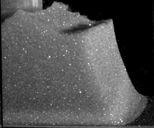
When the gate of the experimental set-up is removed, three different behaviours are observed, depending on the aspect ratio of the column and on the cohesion of the material. When the column is not high enough, it remains static, showing that a minimum height of cohesive material is required to trigger the flow (figure 2a). For a slightly higher column, the material breaks along a well-defined failure plane having its origin at the foot of the pile, leading to the collapse of the top right corner of the column (figure 2b), the rest of the pile remaining undeformed. For a sufficiently high column and/or for a sufficiently weak cohesive force between particles, the collapse starts at the right corner but extends to the bulk, leading to the spreading of the granular mass until a new static configuration is reached (figure 2c). The final deposit surface reveals a roughness reminiscent of undeformed clusters during the flows (Langlois et al. Reference Langlois, Quiquerez and Allemand2015), which increases when increasing the cohesion (Abramian et al. Reference Abramian, Staron and Lagrée2020). In particular, the upper right corner of the initial column seems to be carried by the flow without being sheared or deformed and is present in the final deposit (figure 2c). The same phenomenology is observed in simulations, as shown in figure 2.

Figure 2. Experimental observations (top grey pictures) and numerical simulation (bottom colour pictures) of the collapse of a cohesive granular column. (a) A stable column with small aspect ratio ($a=0.08$, $\ell _c=4.1$ mm, $\ell _c/H_i=0.2$). (b) Partial collapse for a moderate aspect ratio ($a=0.43$, $\ell _c=4.1$ mm, $\ell _c/H_i=0.08$) with a well-defined slip plane. (c) Collapse of the column ($a=1.9$, $\ell _c=2.8$ mm, $\ell _c/H_i=0.025$), where we observe a ‘surfing wedge’ coming from the top right corner being transported during the flow. The white scale bar corresponds to 4 cm in panels (a) and (b), and to 10 cm in panel (c).

However, the origin of the free-surface roughness in the continuous simulations remains unclear and would require a specific study. We observed that the irregularities depend on the mesh size, suggesting that their development might be related to the ill-posed behaviour of the $\mu (I)$ rheology (Barker et al. Reference Barker, Schaeffer, Bohórquez and Gray2015). However, we verified that the dynamics studied in the sequel are independent of mesh size, and calculations were performed with a typical mesh size of $5.86 \times 10^{-3}$ (52 $\mathrm {\mu }$m) in the column.

3.1. Theoretical failure conditions

The failure of hills has been the subject of many studies in the soil mechanics literature (Fredlund & Krahn Reference Fredlund and Krahn1977; Halsey & Levine Reference Halsey and Levine1998; Chen, Yin & Lee Reference Chen, Yin and Lee2003; Duncan, Wright & Brandon Reference Duncan, Wright and Brandon2014). Here, we restrict our analysis to the simple assumption that failure occurs along a straight plane, following the work of Restagno, Bocquet & Charlaix (Reference Restagno, Bocquet and Charlaix2004). The three different configurations depicted in figure 3 are analysed: an infinitely wide rectangular pile, a truncated wide pile and a rectangular pile of finite width.

Figure 3. Theoretical analysis of the stability of columns using a cohesive Mohr–Coulomb criterion. (a) Wide column: the corner delimited by the plane inclined at an angle $\alpha$ is stable when the cohesion level $\ell _c/H_i$ is above the black curve $f_{\theta _c}(\alpha )$ in (3.3). The blue line corresponds to a cohesion level leading to stable column, the red line to a marginally stable column where a single angle $\alpha _m=\theta _c/2+{\rm \pi} /4$ is unstable, and the green line to an unstable column. The grey area corresponds to the unstable angles. (b) Truncated pile: the different curves correspond to the stability function $f_{\theta _c,\theta _m}(\alpha )$ in (3.5) for different values of the free-surface inclination $\theta _m$ (i.e. $\theta _m^1=50^{\circ }$, $\theta _m^2=71.4^{\circ }$, $\theta _m^3=80^{\circ }$). The dashed line is the function $({\ell _c}/{H_i})_{crit}(\theta _m)$ in (3.6) above which the truncated pile is stable. (c) Tall column: the stability curves for various aspect ratios $a$ given by $f_{\theta _c,a}(\alpha )$ in (3.8) for $\alpha < \arctan a$ and by $f_{\theta _c}(\alpha )$ in (3.3) for $\alpha > \arctan a$.

3.1.1. Rectangular pile with a small aspect ratio

We first consider a cohesive rectangular column of height $H_i$ and width $L_i\gg H_i$. A corner delimited by the slip plane having its origin at the bottom right base and inclined at an angle $\alpha$ from the horizontal (figure 3a) is stable according to a cohesive Mohr–Coulomb criterion if the following condition is satisfied:

(3.1)\begin{equation} Mg\sin{\alpha} \leq S \tau_c + \mu_s M g\cos{\alpha}, \end{equation}

where $M$ is the mass of material above the slip plane, $S$ is the area of the failure surface, $\mu _s$ is the static friction angle and ${\tau _c}$ is the cohesive stress. In the configuration of figure 3(a), we can write $M = \rho W {H_i}^2 / (2\tan {\alpha })$ and $S = W H_i /{\sin {\alpha }}$, where $W$ is the thickness of the pile. The pile is then stable when

(3.2)\begin{equation} \frac{\rho g H_i}{2 \tan \alpha}\sin{\alpha}\, (\sin{\alpha} - \mu_s \cos{\alpha}) \leq \tau_c , \end{equation}

which can be expressed using the cohesive length $\ell _c$ and the friction angle $\theta _c=\arctan (\mu _s)$,

(3.3)\begin{equation} f_{\theta_c}(\alpha) = \frac{\cos{\alpha} \sin(\alpha - \theta_c)} {2 \cos{\theta_c}} \leq \frac{\ell_c}{H_i}. \end{equation}

The function $f_{\theta _c}(\alpha )$ is shown in figure 3(a) for $\mu _s=0.4$ corresponding to $\theta _c=21.8^{\circ }$. This function is a symmetric curve centred at $\alpha _m=\theta _c/2 + {\rm \pi}/4$, where it reaches its maximum value $f_{\theta _c}(\alpha _m)\approx 0.17$, and becomes zero for $\alpha =\theta _c$ and $\alpha ={\rm \pi} /2$. In this plot, a point ($\alpha,{\ell _c}/{H_i}$) below the curve corresponds to an unstable corner. A high cohesion level $\ell _c/H_i> 0.17$ corresponds to a stable pile (blue line) for which the stability criterion (3.3) is fulfilled whatever the slip angle $\alpha$. The value $\ell _c/H_i=0.17$ corresponds to the marginally stable pile, which will break along the slip plane inclined at $\alpha _m$ (red line). A low cohesion level $\ell _c/H_i< 0.17$ (green line) corresponds to an unstable column that may fail at any angle for which $f_{\theta _c}(\alpha ) > \ell _c/H_i$ (grey zone in figure 3a).

3.1.2. Truncated pile

The previous analysis can be generalized to the case of a truncated pile, with a missing corner inclined at an angle $\theta _m$ (figure 3b). Studying this geometry is interesting, as it may provide information about the stable final deposit shape. By evaluating the mass of material $M$ located between the slip plane inclined at an angle $\alpha$ and the free surface inclined at an angle $\theta _m$, one can derive the following expression for the stability criterion:

(3.4)\begin{equation} \frac{1}{2}\rho g H_i \left(\frac{1}{\tan \alpha} - \frac{1}{\tan \theta_m} \right) \sin{\alpha}\, ( \sin{\alpha} - \mu \cos{\alpha} ) \leq \tau_c. \end{equation}

Again using $\ell _c$ and $\theta _c$, this equation may be rewritten as

(3.5)\begin{equation} f_{\theta_c,\theta_m}(\alpha) = \frac{\sin(\theta_m- \alpha)\sin(\alpha - \theta_c)}{2 \cos{\theta_c} \sin{\theta_m}} \leq \frac{\ell_c}{H_i} . \end{equation}

The different stability limits in the plane $\alpha$ versus $\ell _c/H_i$ for different truncated angles $\theta _m$ are plotted in figure 3(b). The graphs of the function $f_{\theta _c,\theta _m}(\alpha )$ are curves centred at $(\theta _c + \theta _m)/2$ and vanishing at $\alpha =\theta _c$ and $\alpha =\theta _m$. The rectangular pile is recovered for $\theta _m={\rm \pi} /2$. The maximum of the $f_{\theta _c,\theta _m}(\alpha )$ gives the value of the critical cohesion level $(\ell _c/H_i)_{crit}(\theta _m)$ below which the pile truncated at angle $\theta _m$ is unstable, given by the following equation:

(3.6)\begin{equation} \left(\frac{\ell_c}{H_i}\right)_{crit}(\theta_m)= \frac{1 - \cos(\theta_m- \theta_c)}{4 \cos{\theta_c} \sin{\theta_m}} . \end{equation}

This function $(\ell _c/H_i)_{crit}(\theta _m)$ is plotted in figure 3(b) as the black dashed line. A pile truncated at an angle $\theta _m$ and for a cohesion level $\ell _c/H_i$ such that the point ($\theta _m, \ell _c/H_i$) is below this line, is unstable.

3.1.3. Rectangular pile with a large aspect ratio

The last case of interest is the case when the aspect ratio of the pile is large and such that the slip plane no longer intersects the top free surface but the left side of the pile, i.e. when $\arctan {a} \geq \alpha$ (figure 3c). In this case, $M=\rho W L_i(H_i - \frac {1}{2}L_i\tan \alpha )$ and $S=W L_i/\cos \alpha$, and the stability criterion of the column is given by

(3.7)\begin{equation} \rho g \left( H_i - \frac{L_i \tan{\alpha}}{2} \right) \cos{\alpha} \, (\sin{\alpha} - \mu_s \cos{\alpha}) \leq \tau_c , \end{equation}

which can be written as

(3.8)\begin{equation} f_{\theta_c,a} (\alpha) = \left( 1 - \frac{1}{a}\frac{ \tan{\alpha}}{2} \right) \cos^2{\alpha} \, (\tan{\alpha} - \tan{\theta_c}) \leq \frac{\ell_c}{H_i} . \end{equation}

The stability criterion in this case depends on the aspect ratio $a$ and is given by the function $f_{\theta _c,a}(\alpha )$, which is plotted as curves starting at $(\alpha =\theta _c, 0)$ and presenting a maximum. This maximum increases when increasing the aspect ratio. When the slip angle $\alpha$ reaches the $\arctan {a}$ value, i.e. the slip plane no longer reach the left vertical side of the column, the stability criterion is no longer given by the $f_{\theta _c,a}(\alpha )$ function but by the low-aspect-ratio function $f_{\theta _c}(\alpha )$ in (3.3). For a given aspect ratio $a$, the stability of the column is thus given by a curve made of two parts, as shown in figure 3(c), its absolute maximum giving the critical cohesion level below which the pile is unstable. At low aspect ratio, the first part of the curve (colour curves in figure 3c) is lower than the second part (black curve), and the stability is controlled by a constant cohesion level, independent of $a$. When $a$ becomes greater than 1.145 (black dashed line in figure 3c), the maximum is given by the first maximum corresponding to a mode of failure crossing the pile from one side to another. A stability limit can then be plotted in the $(a, \ell _c/H_i)$ plane, as shown by the black curve in figure 4, separating the stable region (blue) from the region where collapse occurs (pink). The discontinuity between the two geometrical possibilities of failure occurs at $a\approx 1.145$.

Figure 4. Stability diagram in the aspect ratio $a$ versus cohesion level $\ell _c/H_i$ plane for a cohesive granular column. The black curve is the limit of stability. Circles corresponds to experiments, squares to simulation and blue (red) symbols correspond to stable (unstable) columns.

In conclusion, three stability criteria have been derived, depending on the aspect ratio of the rectangular column, or if the pile is truncated with an angle $\theta _m$. In the next section, we test the stability criteria using experimental observations and numerical simulations.

3.2. Experimental and numerical observations

We first investigated experimentally the condition for a collapse of the pile after the opening of the gate. Numerous experiments were done, varying both the aspect ratio $a$ and the cohesive strength $\ell _c/H_i$. The results are plotted in figure 4 as circles, with the following colour code: red indicates that a collapse occurs, and blue indicates that the column remains stable. Experimentally, we were not able to investigate the high-aspect-ratio and large $\ell _c/H_i$ limit, as, for the range of $\ell _c$ accessible with our beads, it would correspond to narrow piles with only few particles in the width.

We can further explore this diagram using numerical simulations. Stable and unstable columns are discriminated by using two criteria: the column is stable either if its final run-out does not exceed 1 % of the initial length, or if the maximum viscosity is reached everywhere in the early stage of the collapse. Overall, these two criteria lead to the same results. The numerical results are data taken from Abramian et al. (Reference Abramian, Staron and Lagrée2020) and data from new computations. The results are plotted figure 4 as squares, with the same colour code as for the circles.

Finally, both experimental and numerical results show a good agreement with the Mohr–Coulomb stability criterion, showing that the limit of stability of a cohesive granular pile is well captured by a simple Mohr–Coulomb model.

5.1. Velocity of the front

Once the gate is removed, the column collapses and a granular front propagates. The profile of the pile during the collapse can be extracted in experiments from the high-speed movie and the laser sheet projection. A typical run is presented in figure 6 showing both the experimental and numerical results for the same parameters for a weakly cohesive material (aspect ratio $a=1$, $\ell _c/H_i=0.0314$). Using the same parameters in simulation (cf. § 2.2), we find a fairly good agreement between the experiments and the numerical predictions for the dynamics of the pile profile during the collapse. The dynamics of the front and its position $L(t)$ can be determined by measuring the location $L(t)$ of the foot of the pile in both experiments and simulations. The experimental results $L(t)-L_i$ are plotted as solid lines in figure 7(a), for $\ell _c=0$ (cohesionless material), $\ell _c=2.8$ mm and $\ell _c=3.6$ mm, for an aspect ratio $a=1$. As a comparison, numerical simulations with the same cohesion levels and the same aspect ratio are plotted with dashed lines. We observe that, after a short acceleration step, the front travels at a constant velocity before decelerating and eventually reaching a static position. The comparison between the experimental and numerical results shows a good agreement from the beginning to the end of the steady state. The agreement is very good for the cohesionless granular experiment (light blue curves), showing that the granular collapse is well described by the continuous numerical code with the $\mu (I)$ rheology. However, in the case of cohesive materials, a difference is observed between experiments and simulation when the flow slows down and stops. The final run-out length is systematically shorter in the numerical simulations for cohesive materials compared to the experiments, as can also be observed in figure 6.

Figure 6. Comparison between the numerical (black) and experimental (blue) profiles of the granular pile at different times for $H_i = 8.9$ cm, $a = 1$ and $\ell _c = 2.8$ mm.

Figure 7. (a) Time evolution of the front position for different cohesion levels in experiments (continuous curves) and simulations (dashed curves) for an aspect ratio $a=1$. Inset: results for $a =0.5$ showing the existence of a significant delay in the experiments before the collapse occurs for the most cohesive material (dark blue, $\ell _c = 3.6$ mm). (b) Velocity of the front $V$ as a function of the aspect ratio $a$ for different cohesion levels. The colour code is the same as in panel (a).

Another discrepancy is observed at lower aspect ratio ($a=0.5$), close to the stability limit (inset of figure 7(a) for a smaller aspect ratio and $\ell _c=3.6\,{\rm mm}$), for which the experiments reveal a delay between the opening of the gate and the initiation of the flow. This delay is not observed in the simulation, and may be reminiscent of more complex rheological features induced by the thick polymer coating, leading to some creeping phenomena not taken into account in the simple rheological model used in the simulation.

Despite this discrepancy, the velocity $V_{max}$ of the front is quantitatively predicted by the simulation, as shown in figure 7(b). The velocity $V_{max}$ is defined as the velocity at the inflection point in the $L(t)-L_i$ curves of figure 7(a). The velocity increases with the aspect ratio up to a plateau when $a\approx 3$. The graph also shows that the velocity decreases when the cohesion increases.

5.2. Run-out and final deposit

Once the kinetic energy of the collapse is fully dissipated, we measure the final deposit and focus on the final run-out length, $L_f=L_i + {\rm \Delta} L$. As shown by Lajeunesse et al. (Reference Lajeunesse, Monnier and Homsy2005), the run-out length and the final height of a cohesionless granular material scale as power laws of the aspect ratio $a$:

(5.1a,b)\begin{equation} \frac{{\rm \Delta} L}{L_i} \propto \left\{\begin{array}{@{}ll@{}} a & \mbox{for } a \leq 3, \\ a^{2/3} & \mbox{for } a \geq 3, \end{array}\right.\quad \mathrm{and}\quad \frac{H_f}{L_i} \propto \left\{\begin{array}{@{}ll@{}} a & \mbox{for } a \leq 0.7, \\ a^{1/3} & \mbox{for } a \geq 0.7. \end{array}\right. \end{equation}

The results for $L_f$ and $H_f$ obtained with cohesionless and cohesive materials are plotted in figures 8(a) and 8(b), respectively, where filled symbols are experimental results and open symbols are numerical results. The run-out length $L_f$ decreases when increasing the cohesion, but the final height $H_f$ remains constant. However, the power laws (5.1a,b) seem unchanged compared to the cohesionless case, as seen by the $a^1$ and $a^{2/3}$ slopes on the graph, although the range of aspect ratio investigated is too narrow to conclude firmly on the scalings. These results are in agreement with previous observations for powders (Mériaux & Triantafillou Reference Mériaux and Triantafillou2008), showing that cohesion only changes the prefactor on the run-out length (5.1a,b), without changing the exponent on the aspect ratio. Unfortunately, understanding this prefactor analytically is not trivial, and is out of the scope of the present paper.

Figure 8. (a) Normalized run-out length ${\rm \Delta} L/L_i$ as a function of the aspect ratio $a$ for different cohesion levels for both experiments and simulations. (b) Normalized height of final deposit $H_f/H_i$ as a function of the aspect ratio $a$.

As discussed previously, the simulations for the cohesive material systematically underestimate the final run-out compared to the experiments. Looking more precisely at the morphology of the free surface at the end of the flow reveals that the discrepancy is localized at the tip of the deposit. The no-slip boundary condition applied in the simulation at the contact line may be a source of additional dissipation explaining the difference between simulation and experiments. We show in the Appendix that, by adjusting the parameters of the rheological model, $\mu _s$, ${\rm \Delta} \mu$ and $I_0$, the run-out can be adjusted, but we found no set of parameters able to predict both cohesionless and cohesive systems.